Clustered Calculation of Worst-Case Execution Times Andreas Ermedahl∗
Friedhelm Stappert†
Jakob Engblom∗
M¨ alardalen Real-Time Research Center Box 883, S-72123 V¨ aster˚ as Sweden
[email protected]
C-LAB F¨ urstenallee 11, 33102 Paderborn Germany
[email protected]
Virtutech Norrtullsg. 15, 11327 Stockholm Sweden
[email protected]
1.
INTRODUCTION
The purpose of Worst-Case Execution Time (WCET) analysis is to provide a priori information about the worst possible execution time of a program before using the program in a system. Reliable WCET estimates are necessary when designing and verifying real-time systems, especially when real-time systems are used to control safetycritical systems like vehicles, military equipment and industrial power plants. WCET estimates are used in real-time systems development to perform scheduling and schedulability analysis, to determine whether performance goals are met for periodic tasks, and to check that interrupts have sufficiently short reaction times. To be valid for use in safety-critical systems, WCET estimates must be safe, i.e. guaranteed not to underestimate the execution time. To be useful, they must also be tight, i.e. avoid large overestimations. A correct WCET calculation method must take into account the possible program flow, like loop iterations and function calls, as well as effects of hardware features, like caches and pipelines. The flow information can be considered as a set of flow facts, each providing a certain piece of information about the program (like loop bounds, infeasible paths, etc.). The expressiveness of the flow facts a calculation method can handle is in high degree determining the WCET estimate precision that can be achieved. In this paper we present a method to handle complex flow information with low computational complexity while still generating safe and tight WCET estimates. We use the key observation that flow facts are usually local in their nature, expressing information that only affects a small region of a program. However, these regions might be larger than the units used in local calculation schemes (a loop nest rather than a loop, or an entire function rather than just a loop inside that function). In general, the boundaries for a flow fact might not agree with the boundaries of a calculation scheme based on the structure of a program. When flow facts cross structural boundaries, and thus calculation boundaries, they cannot be accounted for, which leads to lower precision. One solution to the boundary problem is to work globally on the entire program at once. However, this has a potentially high complexity, and makes scaling to large programs risky. Almost all techniques for performing global calculations are based on integer linear programming (ILP) or constraint programming (CP) techniques, thus having a complexity potentially exponential in the program size. However, by structuring a local calculation after the boundaries dictated by the flow facts, it is possible to achieve both
ABSTRACT Knowing the Worst-Case Execution Time (WCET) of a program is necessary when designing and verifying real-time systems. A correct WCET analysis method must take into account the possible program flow, such as loop iterations and function calls, as well as the timing effects of different hardware features, such as caches and pipelines. A critical part of WCET analysis is the calculation, which combines flow information and hardware timing information in order to calculate a program WCET estimate. The type of flow information which a calculation method can take into account highly determines the WCET estimate precision obtainable. Traditionally, we have had a choice between precise methods that perform global calculations with a risk of high computational complexity, and local methods that are fast but cannot take into account all types of flow information. This paper presents an innovative hybrid method to handle complex flows with low computational complexity, but still generate safe and tight WCET estimates. The method uses flow information to find the smallest parts of a program that have to be handled as a unit to ensure precision. These units are used to calculate a program WCET estimate in a demand-driven bottom-up manner. The calculation method to use for a unit is not fixed, but could depend on the included flow information and program characteristics.
Keywords WCET analysis, WCET calculation, hard real-time, embedded systems. ∗ This work is performed within the Advanced Software Technology (ASTEC, www.docs.uu.se/astec) competence center, supported by the Swedish National Board for Industrial and Technical Development (NUTEK, www.nutek.se). † Friedhelm is a PhD student at C-LAB (www.c-lab.de), which is a cooperation of Paderborn University and Siemens.
Permission to make digital or hard copies of all or part of this work for personal or classroom use is granted without fee provided that copies are not made or distributed for profit or commercial advantage and that copies bear this notice and the full citation on the first page. To copy otherwise, to republish, to post on servers or to redistribute to lists, requires prior specific permission and/or a fee. CASES’03, Oct. 30–Nov. 2, 2003, San Jose, California, USA. Copyright 2003 ACM 1-58113-676-5/03/0010 ...$5.00.
1
hancing features, like caches and pipelines. Low-level analysis can be further divided into global low-level analysis, for effects that require a global view of the program, and local low-level analysis, for effects that can be handled locally for an instruction and its neighbours. In global low-level analysis, instruction caches [15, 13, 19, 20, 29], data caches [17, 29, 31], and branch predictors [5, 23] have been analyzed. Local low-level analysis has dealt with scalar pipelines [5, 6, 7, 10, 13, 20, 22, 29] and superscalar CPUs [21, 28]. Heckmann et al. [15] present an integrated cache and pipeline analysis, and argue that such integration is necessary for processors with heavy interdependencies between various functional elements. Attempts have also been made to use measurements and the hardware itself to extract the timing [26]. The purpose of the calculation phase is to calculate the WCET estimate for a program, combining the flow and timing information derived in the previous phases. There are three main categories of calculation methods proposed in literature: tree-based, path-based, and IPET (Implicit Path Enumeration Technique). In a tree-based approach, the WCET is calculated in a bottom-up traversal of a tree generally corresponding to a syntactical parse tree of the program, using rules defined for each type of compound program statement (like a loop or an if-statement) to determine the WCET at each level of the tree [3, 4, 5, 20]. The method is conceptually simple and computationally cheap, but has problems handling flow information, since the computations are local within a single program statement and thus cannot consider dependencies between statements. In a path-based calculation, the WCET estimate is generated by calculating times for different paths in a program, searching for the overall path with the longest execution time [13, 29, 30]. The defining feature is that possible execution paths are explicitly represented. The path-based approach is natural within a single loop iteration, but has problems with flow information stretching across loop-nesting levels. In IPET, program flow and low-level execution time are modeled using arithmetic constraints [8, 11, 16, 19, 25, 27]. Each basic block and program flow edge in the program is given a time variable (tentity ), and a count P variable (xentity ), and the WCET is extracted by maximizing i∈entities xi ∗ti , where the xi are subject to constraints reflecting the structure of the program and possible flows. The result is a worstcase count for each node and edge. As shown in [8], very complex flows can be expressed using constraints, but the computational complexity of solving the resulting problem is potentially very high, since the program is completely unrolled and all flow information is lifted to a global level. Both the path-based and tree-based calculation methods are performed in a bottom-up fashion. Bottom-up calculation methods calculate a safe (timing) abstraction for a part of the program, which is later used in the calculation of surrounding parts of the program. For the tree-based calculation the abstraction unit is a program statement, while for the path-based calculation it is a loop or a function. Bottomup calculations are beneficial, since the overall WCET calculation problem can be subdivided into smaller easier-to-solve problems. At the other extreme we have the IPET methods, where no subdivision is made and the unit of calculation is the entire program.
efficient local calculation and high precision, since all facts can thus be accounted for while still avoiding the need for global calculation (unless there are actual flow facts that make this necessary). Another key observation is that in many cases it is not sufficient to consider each provided flow fact in isolation. Many different types of flow facts might be generated for the same program and such flow facts can interact and together constrain program flow in a manner not possible by single flow facts. A WCET calculation method working over smaller program parts therefore must, to achieve maximum precision, find interacting flow facts and treat them as a unit. This is achieved by our clustered calculation, which basically works as follows: The provided flow information is used to construct units where the included flow facts all have to be considered together. For each such fact cluster the part of the program covered by the included flow facts is extracted. The fact clusters and corresponding program parts are used to calculate a program WCET estimate in a demand-driven bottom-up manner. The calculation method to use for a particular fact cluster is not fixed, but could depend on the characteristics of the included flow facts and corresponding program parts. The concrete contributions of this paper are: • We introduce the concept of organizing flow information into fact clusters. • We present various algorithms to construct fact clusters. • We present an algorithm that uses fact clusters to calculate a program WCET estimate. • We evaluate the clustered calculation method against global and local calculation schemes. The rest of this paper is organized as follows: Section 2 introduces previous work, Section 3 presents our WCET tool architecture, and Section 4 presents our flow representation for WCET analysis. Section 5 presents how flow facts can be organized into fact clusters, and Section 6 gives the clustered WCET calculation method. Section 7 presents different calculation alternatives. Section 8 gives an illustrating example of the clustered calculation method. Finally, Section 9 presents our experimental evaluation, and Section 10 gives our conclusions and ideas for future work.
2. WCET ANALYSIS OVERVIEW To generate a WCET estimate, we consider a program to be processed through the phases of flow analysis, low-level analysis and calculation. The purpose of the flow analysis phase is to extract the dynamic behaviour of the program. This includes information on what functions get called, how many times loops iterate, if there are dependencies between if-statements, etc. Since the flow analysis does not know the execution path which corresponds to the longest execution time, the information must be a safe (over)approximation including all possible program executions. The information can be obtained by manual annotations (integrated in the programming language [18] or provided separately [8, 11, 19]), or by automatic flow analysis [12, 13, 16, 22, 29]. The purpose of low-level analysis is to determine the timing behaviour of instructions given the architectural features of the target system. For modern processors it is especially important to study the effects of various performance en2
Manual annotations Input data specification
WCET tool Flow analysis
Scope graph with flow info
Scope graph with flow and exec info
Cache analysis (global)
Local WCET
Pipeline analysis (local)
Program source Input data Data Processing module
Timing model Compiler
Object code
Fact cluster generation
Simulator
Fact clusters Scope graph traversal
Fact cluster IPET- or pathand covered based WCET scopes calculation Cluster-based calculation WCET
Figure 1: WCET tool architecture sequence [6, 7, 30]. These timing effects are usually negative due to the pipeline overlap between the two nodes. Timing effects reaching across node sequences longer than two are also taken into account where necessary. This timing model is powerful enough to capture the effects of pipelines and caches, separating the analysis of machine aspects from the calculation phase. It is also not tied to our particular fashion of low-level analysis. For example, the integrated cache and pipeline analysis for the Motorola ColdFire 5307 processor presented by Ferdinand et al. [10] generates a model where times are assigned to basic blocks in a program (including the effect of both pipelines and caches on the timing of each block). Such a timing model can be used within our framework, with the clustered calculation method presented in this paper. Similarly, the timing model for Infineon C167 presented by Atanassov et al. [1] attributes times only to edges in the flow graph, and this model would also fit in our timing model framework.
In this paper we present an approach where the part of the program calculated locally is not predetermined statically but depends on the flow information available for the program. The calculation is performed bottom-up, but is demand-driven in that a WCET for a program part is only calculated when its timing estimate is needed in a surrounding program part.
3. TOOL OVERVIEW AND TERMINOLOGY The work presented in this paper is implemented within the framework of our existing WCET analysis tool. In addition to previous implemented extended IPET-based [8, 9] and path-based [9, 30] calculation methods, we have implemented a calculation module based on clustering. Figure 1 gives an overview of the WCET tool, when using a clustered calculation module (as presented in this paper). Compared to our previously presented work [8, 30] all components of the system except the calculation phase remain unchanged, demonstrating the modular structure of the tool. The modular architecture allows independent replacement of the modules implementing the different steps, which makes it easy to customize a WCET tool for particular target hardware and analysis needs. All data structures and analysis phases in our WCET tool are based on the possibility of partitioning the instructions in the object code into basic blocks 1 . Figure 2(a) shows an example C function, Figure 2(b) and Figure 2(c) show the corresponding assembler code and basic block graph. We have an automatic flow analysis currently under development [12]. The flow analysis results in a description of the dynamic behaviour of the program, consisting of a scope graph annotated with flow facts (Figure 2(d)), as described in more detail in Section 4 below. For the current experiments, we rely on a machine model for a NEC V850E [6, 7] that accurately models a processor pipeline using a trace-driven cycle-accurate simulator. For the V850E target, caches are not used. The nodes in the scope graph can be annotated with additional execution information, e.g. giving what instructions that will hit or miss the cache and the type of memory being accessed [6, 9] (not explicitly shown in Figure 2(e)). The resulting timing model, see Figure 2(f), is a data structure containing times for each entity (node or edge) in the scope graph. Times for nodes correspond to the execution times of basic blocks (with additional execution information) in isolation , e.g. tA in Figure 2(f), and times for edges, e.g. δAC in Figure 2(f), to the timing effect when two successive nodes are executed in
4.
REPRESENTING PROGRAM FLOW
The scope graph is a hierarchical representation of the dynamic behaviour of a program suitable for WCET analysis. The graph consists of nodes and edges where each node is referring to a basic block in the object code. A basic block might be referenced by several different scope nodes. The nodes and edges in the scope graph are partitioned into scopes reflecting the dynamic structure of the program in terms of function calls, loops, recursive calls and unstructured code parts. Scopes are necessary in order to carry program flow information, in particular bounds for all loops and context-sensitive flow information for function calls. Figure 2(d) shows the scope graph generated for the code in Figure 2(a). Each scope has a distinguished header node, (e.g. node A resp. C in Figure 2(d)), with the property that no other node in the scope can be executed more than once without passing the header node. Each scope should have a loop bound attached to it, providing an upper bound on the number of times its header node can be executed for each entry of the scope. The scopes in the scope graph are organized in a scopehierarchy, a directed tree with scopes as vertices and edges from a scope going to all its children. Figure 2(e) illustrates the scope-hierarchy generated for the scope graph in Figure 2(d). In the tree each scope has zero or more descendants, i.e. scopes below it in the tree, and zero or more ancestors, i.e. scopes above it in the tree. The immediate descendants of a scope are its child scopes and the immediate ancestor is its parent scope. A scope without any descendant is called a leaf scope. E.g. in Figure 2 scope loop is a
1
A basic block is a maximal sequence of instructions that can be entered only at the first instruction in the sequence and exited only at the last instruction in the sequence [24]. 3
(a) C source code
start
mov movi mov br foo_0: add addi addi foo_1: cmp blt foo_2: cmpi bge foo_3: addi foo_4: cmp bge foo_5: mov jmp
r0,r6 #1,r7 r0,r5 foo_1 r7,r5 #-2,r5 #1,r6 r6,r1 foo_5
foo:
foo
foo:
foo_0: foo_1:
A
C
foo_2:
#5,r6 foo_4
scope: foo; header: A; loopbound: 1;
foo:
loop
int foo(int max) { int i,j,total; i = 0; j = 1; total = 0; while(i max) break; total = total + j - 2; i++; } return total; }
B
foo_0:
scope foo scope: loop; header: C; loopbound: 10; loop::#E=1; loop:[ ]:#E £ 5;
foo_1:
D
foo_2:
foo_3:
E
tA= 8 A
foo_3:
dAC= -1
scope loop loop::#E=1; loop:[ ]:#E £ 5;
B tB= 6 C
tC= 5
dFB= -1
dBC= -1 dCD= -1 D
dCG= -2
E
#1,r7 r7,r1 foo_0 r5,r1 [31]
(b) Assembler code
F
foo_4:
G
foo_5: (c) Basic block graph
F
foo_4:
tG= 5
foo_5:
exit
(d) Scope graph and flow facts
(e) Scope hierarchy with flow facts
tD= 4 dDE= -1
G
tE= 5
dEF= --2 tF= 4
dFG= -2
(f) Timing model
Figure 2: WCET analysis stages or [min..max], where min ≤ max are integers larger than 0. The constraints are specified as a relation between two arithmetic expressions involving execution count variables and constants. An execution count variable, #entity, corresponds to an entity (node or edge) in the scope graph, and represents the number of times the entity is executed in the context given by the context specification. A fact can only refer to count variables corresponding to entities located in the complete subtree of the defining scope of the fact. For example, a fact defined in scope loop cannot refer to executions of entities located in the foo scope. All scopes between the defining scope and the scopes containing referred count variables are said to be covered by the fact. Thus, the scopes covered by a fact form a subtree with the defining scope as root. For each scope covered by a fact the fact spans a number of iterations. For the defining scope the span is the number of iterations specified by the context specifier. For all other covered scopes the span is all iterations of the scope. In Figure 2(d), the loop scope has two flow facts attached to it. The first flow fact specifies that for each time loop is entered, node E must be taken during each of the first five loop iterations (but not that the loop needs to iterate 5 times). The second fact specifies that for each time loop is entered node E can be taken at most five times. Observe that the facts are local to scope loop, and should be valid for each entry of the loop, independently on how many times function foo is called from other functions in the program.
descendant and a child to scope foo. Scope loop is also a leaf scope. The complete subtree for a scope s is formed by all scopes having s as ancestor in the scope-hierarchy (including s). Each tree of scopes formed by removing the complete subtrees of one or several descendant scopes of s is a subtree of s. An in-edge of a scope s is an edge having its source node in a scope not within the complete subtree of s and having its target within the complete subtree of s. An in-node is a target node of an in-edge. An out-edge of a scope s is an edge having its source node in a scope within the complete subtree of s and having its target outside the complete subtree of s. Timing effects reaching across scope boundaries are always taken into account via out-edges. That is, the timing effect associated with an out-edge of a scope s is included in the timing calculation of s, and, vice versa, the timing effect of an in-edge of s is taken into account by the calculation of the corresponding source scope. A scope can be entered at several in-nodes, allowing for unstructured jumps into loops, and might have several out-edges. An edge going to a header node of a scope s and having its source node located in the complete subtree of s is a back-edge of s. E.g. in Figure 2(d) A→C is an in-edge, F→G an out-edge and B→C a back-edge of scope loop.
4.1 Flow facts To express more complex program flow information than just basic loop bounds each scope can carry a set of flow facts [8, 9]. The flow facts combine the expressive power of IPET, using constraints to limit possible executions of scope graph entities, with the ability to give the flow information in a scope-local context. Each flow fact consists of three parts: the name of the defining scope where the fact is attached, a context specifier, and a constraint expression (see Figure 2(d)). Each flow fact is considered local to its defining scope and the fact is interpreted as being valid for each entry of the scope. The context specifier describes the iterations for which the constraint expression is valid. This can be for all iterations or for just some iterations. The type of a context specification is either total (written with “[” and “]”), for which the fact is considered as a sum over all iterations of the specified scopes, or foreach (written with “”), which considers the fact as being local to a single iteration of the scope. Facts valid for all iterations are expressed by “” or “[]”, while facts valid for certain iterations are expressed as
5.
CLUSTERING OF FLOW FACTS
The goal of clustering is to find the flow facts that need to be considered together in order not to lose precision. Such interacting flow facts are caused by facts sharing application area with some other facts, by reaching down into descendant scopes and by having overlapping range specifications. Together the flow facts also indirectly specify a part of the scope graph that needs to be considered together with the flow information in the calculation. We define a fact cluster to be a set of flow facts. The defining scope of a fact cluster is defined to be the first common ancestor of all the facts in the cluster. The cover of a fact cluster is all scopes between the defining scope and the scopes containing count variables referred to by a flow fact in the scope. Thus, the covered scopes form a subtree 4
n:[1..5]:#N1 £ #N2+2 (f1) n::#N1+ #N3 =1 (f2)
void foo(bool x) { if( cond ) x = true; for( ... ) for (... ) if( x ) Q1 }
scope m m::#M1£ #Q1 (f4)
scope n
scope p
scope q scope o o::#O2 N3 = 0 (f3)
r:[]:#header(s) £ 55 (f5) scope r scope s
s::#S1 = 1 (f6)
(a) Example scope-hierarchy with associated facts Fact Defining Span def Covered scope scope scopes
f1 f2 f3 f4 f5 f6
n {n} 1..5 n 3..7 {n} o 8..10 {o} m 1..lb(m) {m,p,q} r {r,s} 1..lb(r) 1..5 s {s} (b) Information about facts
Fact cluster
{f1,f2} {f3} {f4} {f5,f6} {f6}
Defining Span def scope scope
n o m r s
1..7 8..10 1..lb(m) 1..lb(r) 1..5
// Block M1 // Outer loop, (scope p) // Inner loop, (scope q) // Block Q1, execution implied by M1
Figure 5: Long reaching dependency Covered scopes
example if the outcome of a decision in a scope determines the paths taken in a loop (maybe deeply) nested in the scope (with varying outcome), like e.g. for the scopes m, p and q in Figure 3(a). Figure 5 shows example code with such a long reaching dependency. Flow fact f4 in Figure 3(a) captures this type of nested dependency. It gives that an execution of M1 implies an execution of Q1, (node Q1 can still be executed on its own).
{n} {o} {m,p,q} {r,s} {s}
(c) Information about fact clusters
Figure 3: Fact clustering example
for( ... ) { if( cond ) { N3; break; } ... }
in the scope-hierarchy with the defining scope as root. For the defining scope s of a cluster the span is all iterations between the lowest and highest iteration of s spanned by any fact in the cluster. For all other covered scopes the span is equal to all iterations of the scope. In Figure 3(a) an example scope-hierarchy with associated flow facts is given. In Figure 3(b) we show the defining scopes, defining scope spans, and cover of each given flow fact. The name of a referred count variable gives the scope in which the corresponding entity is located, e.g. #N1 refers to executions of node N1 located in scope n. The function lb(s) returns the loop bound for a scope s. The fact clusters generated from the facts are given in Figure 3(c). For each generated fact cluster we show its defining scope, its defining scope span, and the scopes covered by the cluster. Note that the same flow fact can be present in several clusters, and that not all flow facts in a cluster need to have the same defining scope.
// Bound: 10, (scope o) // Block 02, false during last 3 iters // Block N3, big chunk of work
Figure 6: Condition dependent dependency In the next example, shown in Figure 6, block N3 does not belong to the loop (due to the break statement), and the way the loop is exited will determine whether it should be counted or not. Thus, N3 depends on the decision cond in the loop body, but N3 is a node in the parent scope of o (scope n). Fact f3 in Figure 3 captures this dependency by specifying that the edge O2→N3 can not be taken during the last three iterations of the o scope. Another case of flow information causing clusters is when information from different types of flow analysis methods or manual annotations interact, and therefore need to be considered together in the WCET calculation. An example of such overlapping flow information is shown in Figure 3(a) with flow facts f1 and f2. Both flow facts have the same defining scope n and they overlap in the ranges of their context specifications.
5.1 Flows causing clusters Program flows causing fact clusters and reaching over several scopes are actually quite common. The simplest example is illustrated in Figure 4. It is the classical “triangular” loop, i.e. a nested loop where the number of iterations of the inner loop depends on the current iteration number of the outer loop (cf. scopes r and s in Figure 3(a)). for(i=0; i