The input vectors for the following analysis consisted of 47 spectral ..... [12] Ultsch, A; Siemon, HP; Exploratory Data Analysis: Using Kohonen Networks.
Clustering of EEG-Segments Using Hierarchical Agglomerative Methods and Self-Organizing Maps David Sommer, Martin Golz University of Applied Sciences, Department of Computer Science, Postfach 182 D-98574 Schmalkalden, Germany {sommer, golz}@informatik.fh-schmalkalden.de
Abstract. EEG segments recorded during microsleep events were transformed to the frequency domain and were subsequently clustered without the common summation of power densities in spectral bands. Any knowledge about the number of clusters didn’t exist. The hierarchical agglomerative clustering procedures were terminated with several standard measures of intracluster and intercluster variances. The results were inconsistent. The winner histogram of Self-organizing maps showed also no evidence. The analysis of the U-matrix together with the watershed transform, a method from image processing, resulted in separable clusters. As in many other procedures the number of clusters was determined with one threshold parameter. The proposed method is working fully automatically.
1
Introduction
Eleven subjects (3 females, 8 males), aged 19 to 36 years, participated in an overnight driving simulator study. Their task was intentionally monotonous, simply to avoid major lane deviations. Electrooculogram (EOG, oblique) and electroencephalogram (EEG) were recorded in two unipolar and two bipolar recordings. Dangerous short attention-loss phases during driving are characterized by a transition from struggling to remain awake to an involuntary short sleep episode. These phases, sometimes called microsleeps [1], are associated in many cases with an increased activity of slow eye movements (SEM) [2, 3]. The EEG during SEM, as in the whole transition phase from drowsiness to sleep, was found to have much more complex and variable patterns than the wakeful EEG [2]. Our investigations were focused on clustering the spectral features of the EEG during the SEM, to show if there are differences in EEG indicative of different functional states of the brain.
2
Clustering with agglomerative hierarchical methods
The input vectors for the following analysis consisted of 47 spectral components (2 to 25 Hz; 0.5 Hz steps). A principal component analysis (PCA) was routinely computed,
but there was no reason to assume input vectors in a linear subspace, because the last ten principal components had a residual variance of approximately 8%. A Scree test and the Kaiser criteria for the covariance matrix (number of eigenvalues greater than one) indicated 13 principal components, but they explained only 30% of the total variance. Therefore, all 47 variables were included in a cluster analysis, performed with the SAS package [4]. Five different agglomerative procedures were applied (Tab. 1) and were terminated with six different measures. The measures, except the elbow measure, are based on estimates of the intracluster and intercluster variances and are all implemented in SAS. In [5] 24 different measures were applied to data sets with known numbers of clusters. The measure with the best reliability was ‘Pseudo-F’.
Table 1. Estimated numbers of clusters obtained from five different agglomerative hierarchical methods with six different measures. Left: for the standardized data set. Right: for the nonstandardized data set.
The estimated numbers of clusters were inconsistent (Tab. 1) depending on the method used on the termination measure and on the data set. We used two data sets, one without and one with standardization of the data, recommended by several authors [6, 7]. A number of clusters greater than 12 was excluded, because it is difficult for an EEG-expert to interpret such a large number of clusters.
Fig. 1a. Dendrogram of the Average Linkage method for the non-standardized data set
Fig.1b. Dendrogram of the Ward method for the non-standardized data set
With the Centroid method, an indication of seven clusters was found in all six measures using both data sets. Using the Ward method, six clusters were found in 5 of
the 6 measures in the non-standardized data set only. In the standardized data set, three clusters were found in only three of the measures. The dendrograms obtained for three linkage methods showed a lot of very small clusters (Fig. 1a). Dendrograms without such miniclusters were computed for Centroid and Ward methods (Fig. 1b). A factor analysis using Varimax rotation prior to clustering led to a reduction to 13 variables. But all subsequently applied agglomerative methods achieved higher inconsistencies in the number of clusters compared to the analysis of original input vectors. The simple model underlying all measures for terminating the agglomerative process is disadvantageous. Specifically, the linkage methods are not well characterized with variance measures.
3
Clustering with SOM
The self-organizing feature map (SOM) [8] was applied to the non-standardized data set for clustering. Using the principle of competitive learning, the weight vectors can be adapted to the probability density function of the input vectors [9]. The similarity between the input vector x, and the weight vector w, was calculated by the Euclidian distance. During training an arbitrary weight vector wj was updated at iteration index t by: ∆Z
=�η�W �K
�W �
�
�W �>[ �W � Z �W @
(1)
Where η(t) is a learning rate factor decreasing during training, and hcj(t) is a neighborhood function between wc, the weight vector winning the competition, and the weight vector wj. hcj(t) is also decreasing during training. The neighborhood relationships are defined by a topological structure and are fixed during training. We used a two-dimensional tetragonal relationship. In the final phase of training, the fineadjustment [9], the neighborhood radius is very small, leading to updates of the winning weight vectors wc and of their nearest neighbors. For a one-dimensional topological structure it can be shown [9] that the training rule Eq. (1) leads to an approximation of a monotonous function of the probability density function of the input vectors. The two-dimensional topology results in a compromise between a density approximation and a minimal mean squared error of vector quantization [10]. In the case of existing compact regions of input vectors and of existing density centers, as for Gaussian mixtures, the evaluation of the relative winner frequency of the neurons leads to a visualization of clusters. Fig. 2a shows such a gray-level-coded winner histogram. Five areas with increased winner frequency are evident. The Gaussian mixture data were generated by fixing five cluster centers and five covariance matrices, and adding normal distributed noise in a 47-dimensional space, as in our experimental data set. The size of the generated data set and of the experimental data set was equal, and their estimated total covariance matrices were approximately equal. The black colored units in Fig. 2a are dead neurons, which make it easy to separate clusters. Fig. 2b shows the relative winner frequency for the
experimental data set. A separation of regions with increased winner frequency is not possible.
Fig. 2a. Relative winner frequency for a SOM with 30x40 neurons for Gaussian mixture data
Fig. 2b. Relative winner frequency for a SOM with 30x40 neurons for SEM-EEG data
For a topology-preserving mapping neighbored, weight vectors in input space are also neighbored in output space (the two-dimensional map) [11]. The mapping from input to output space is quasi-continuous, but must not be continuous in the reversed direction. Therefore, two topologically neighbored weight vectors must not represent one cluster. If their distance is small, then they probably represent one cluster, otherwise they probably represent different clusters. The visualization of the distances between neighbored weight vectors was introduced as the unified distance matrix (U-matrix) [12]. In the following, only two-dimensional tetragonal topologies are considered. For every weight vector wx,y, where x and y are the topological indices, the Euclidian distances dx and dy between two neighbors and the distance dxy to the next but one neighbor is calculated:
dx (x, y ) = w x, y − w x +1, y dy (x, y ) = w x, y − w x, y +1 dxy(x,y ) =
w x,y +1 − w x +1,y 1 w x,y − w x +1,y +1 + 2 2 2
(2)
The distance du was calculated as the mean over eight surrounding distances. With the four distances for each neuron dx, dy, dxy and du, the U-matrix is well defined and has the size (2nX -1) x (2nY - 1) (Fig. 3). In Fig. 4 the U-matrix elements were mapped on a gray scale. Light-gray levels indicate low values, and dark-gray levels indicate high values. Visual scoring of five clusters in the U-matrix of Gaussian mixture data (Fig. 4a) is evident. As expected, the cluster regions on the map are regions of small distances between the weight vectors, which are separated by small regions of large distances.
The U-matrix of the SEM-EEG data (Fig. 4b) has much more complexity and it is difficult to define borders. du(1,1) ( ) dy 1,1 U = du(1,2) dy(1,2) du 1,ny �
( )
dx(1,1) dxy(1,1)
dx(1,2) dxy(1,2) �
( )
dx 1,ny
du(2,1) dy(2,1)
du(2,2) dy(2,2) �
( )
du 2,ny
�
du(nx ,1) dy(nx ,1) du(nx ,2) dy(nx ,2) du nx ,ny �
(
)
du
dx
dy
dxy
Fig. 3. Definition of the U-matrix and localization on the tetragonal topological structure, shown for the neuron in the center only. Circles: positions of neurons; black squares: positions of U-matrix elements
Fig. 4a. U-matrix for SOM from Fig. 2a
Fig. 4b. U-matrix for SOM from Fig. 2b
Costa et al. [13] propose an automatic segmentation of the U-matrix using the watershed algorithm of gray scale image processing [14]. Regarding high values as mountains and low values as valleys, the algorithm can be illustrated by flooding the valleys with water; watersheds will be built up where the water converges (Fig. 5a). This algorithm leads to closed borders. All weight vectors in one segmented region represent one cluster, and the fusion of their Voronoi sets leads to all items of a cluster. The results of segmentation are dependent on the size of the SOM. With a relatively large number of weight vectors, many clusters are obtained. Smoothing the gray level function with a two-dimensional filter reduces the risk of oversegmentation; here a 3x3-gaussian filter was applied. The size of the SOM was considerably restricted when the topographic product [15] was taken into account. The topographic product is a measure for the correspondence of the input and output space dimensions. We obtained an optimal value for a SOM size of 4 x 6, but in the case of such small maps the segmentation of the U-matrix failed. Therefore, we extended the size but retained the ratio of approximately 70%. On the other hand, it was shown, that the topographic product was a good measure for approximately linear manifolds only [11].
Watershed
Reservoir
Minima
Fig. 5a. Cross section of gray scale mountains
Fig. 5n. U-matrix from Fig. 4b after watershed transformation
In several regions of the U-matrix (Fig. 5a, 5b) black-and-white textures are observable. They describe relatively large differences between dx and dy, and are connected with local stretchings of the SOM along one topological coordinate. If, on the other hand, the dx-elements of the U-matrix, for example, are visualized only, some segment borders disappear. Therefore we restricted our investigations to the function du(x,y).
Fig. 6a. Number of clusters vs. hmin for the U-matrix of Fig. 5b with generation of new regions [13].
Fig. 6b. The same as in Fig. 6a but without generation of new regions
Flooding the reservoirs has to be started at an initial level hmin [14]. It was not straightforward to find suitable values for hmin. Starting with hmin = Umin = min( du(x,y) ), the global minimum, as well as with to high values for hmin led to one cluster only. With a given value hmin the number of clusters is fixed and is preserved during flooding. The number of clusters versus hmin showed no plateau (Fig. 6a), however, distinctive plateaus are required to get a reliable number of clusters [13]. Therefore, we propose a modification allowing the generation of new minima regions during flooding. All local minima regions of the function du(x,y) with values greater than hmin are considered as autonomous clusters. To avoid over-segmentation only significantly extended regions were taken into account. Such regions could correspond to clusters with lower probability densities.
Under this modification an extended plateau was calculated at 9 clusters (Fig. 6b). The assumption of 10 clusters is misleading because hmin can not be below the global minimum Umin.
Fig. 7. All 1652 input vectors grouped in 9 different clusters; horizontal: frequency; vertical: item; gray scale: spectral power density.
4
Results
The 9-cluster solution of the described automatic clustering and segmentation procedure is shown in Fig. 5b. The segments contain different numbers of weight vectors. The fusion of their Voronoi sets, mentioned above, leads to the clusters (Fig. 7). Cluster 1 and 2 contain input vectors with large magnitudes in the alpha1 band (7.5-10.5 Hz), cluster 6 in the alpha2 band (10.5-12.5 Hz), cluster 3 in the theta band (3.5-7.5 Hz) and cluster 9 in the delta band (1.0-3.5 Hz). In contrast to the usual summation in frequency bands, greater detail can be seen. The input vectors of cluster 1 and 2, for example, are large in the same spectral band, but they differ in the magnitude range and differ in other spectral bands. From Fig. 7 one may get the visual impression of homogeneous clusters, with the exception of cluster 7 and 8. The described method is working fully automatically and has a low number of free parameters. Beside the common parameters for the SOM, there is only one parameter hmin for segmentation. Clustering is possible with a high reproducibility. Many reruns with 80% of all input vectors, arbitrary selected, lead to always nine clusters. With the proposed segmentation method, a visualization of the SOM is not necessary and the limitation to two-dimensional maps can be left behind. It is possible to extend the whole clustering method to higher dimensional topologies.
References [1] Thorpy, MJ; Yager, J; The Encyclopedia of Sleep and Sleep Disorders; NewYork: Facts on File, 1991. [2] Santamaria, J; Chiappa, KH; The EEG of Drowsiness in Normal Adults; J Clin Neurol; 4 (4), 1987, 327-382. [3] Liberson, WT; Liberson, CT; EEG recordings, reaction times, eye movements, respiration and mental content during drowsiness; Proc Soc Biol Psychiat, 19, 1966, 295-302. [4] SAS Institute Inc., SAS/STAT User’s Guide, Version 6, Fourth Edition, Volume 1, Cary, NC: SAS Institute Inc., 1989, 943 pp. [5] Milligan, GW; Cooper, MC; An examination of procedures for determining the number of clusters in a data set; Psychometrika, 50 (2), 1985, 159-179. [6] Deichsel, G; Trampisch, H; Clusteranalyse und Diskriminanzanalyse; Gustav Fisher Verlag, Stuttgart, 1985. [7] Backhaus, K; Erichson, B; Plinke, W; Weiber, R; Multivariate Analyseverfahren; (6. Aufl.), Berlin, Heidelberg, New York.Springer, 1996. [8] Kohonen, T; Self-organized formation of topologically correct feature maps; Biol Cybern, 43, 1982, 59-69. [9] Kohonen, T; Self-Organizing Maps; 3rd edition, Springer, Berlin, 2000. [10] Fritzke, B; Wachsende Zellstrukturen – ein selbstorganisierendes neuronales Netzwerkmodell; PhD thesis; University of Erlangen, 1992 (in german). [11] Villmann, T; Topologieerhaltung in selbstorganisierenden neuronalen Merkmalskarten; PhD thesis, University of Leipzig, 1996 (in german). [12] Ultsch, A; Siemon, HP; Exploratory Data Analysis: Using Kohonen Networks on Transputers; Univ. of Dortmund, Technical Report 329, Dortmund, Dec. 1989. [13] Costa, JAF; Netto, MLA; Estimating the Number of Clusters in Multivariate Data by Self-Organizing Maps; Int. J Neural Systems, 9 (3), 1999, 195-202. [14] Vincent, L; Soille, P; Watersheds in Digital Spaces: An Efficient Algorithm Based on Immersion Simulation; IEEE Transaction on Pattern Analysis and Machine Intelligence, 1991. [15] Bauer, HU; Pawelzik, KR; Quantifying the neighborhood preservation of SelfOrganizing Feature Maps. IEEE Trans. Neural Networks, 3 (4), 1992, 570-579.