IEEE GEOSCIENCE AND REMOTE SENSING LETTERS, VOL. 2, NO. 1, JANUARY 2005
59
Hierarchical Clustering of Multispectral Images Using Combined Spectral and Spatial Criteria André R. S. Marçal and Luísa Castro
Abstract—An agglomerative hierarchical clustering method, which uses both spectral and spatial information for the aggregation decision, is proposed here. The method is suitable for large multispectral images, provided that an unsupervised classification is previously applied. The method is tested on a synthetic image and on a satellite image of the coastal zone. Index Terms—Clustering methods, image classification, image processing, image region analysis.
I. INTRODUCTION
A
LARGE number of multispectral images of the earth are acquired daily by the current remote sensing satellites. Consistent automatic data exploration tools are increasingly required in order to make use of the huge volumes of data made available. Clustering and unsupervised classification methods are powerful techniques that can be used to reveal structures and to identify “natural” groupings on the image data. Hierarchical methods are needed if we seek to reveal structure in the data at many levels [1]. This is a convenient approach when it is not clear how many and which classes are present in the data. Hierarchical clustering techniques proceed by either a series of successive mergers or a series of successive divisions [2]. Agglomerative hierarchical methods start with individual objects, or pixels on a digital image. This is a major limitation, as usually satellite images will be too big (typically millions of pixels) for such a method to be computationally viable on a pixel by pixel basis. An alternative way is to use an agglomerative hierarchical method after the application of some other clustering method. For example, the Isodata method [3] can be used to classify the image into a reasonably small number of classes (e.g., 40). The resulting classes from this initial classification are then clustered hierarchically, providing a dendogram that will then allow for various levels of discrimination to be extracted from the image data. One problem of this approach is that the final results are strongly dependent both on the unsupervised classification and on the hierarchical clustering method. Usually the hierarchical clustering criterion is based exclusively on the spectral information of each object, in this case a set of image pixels or class. A more meaningful result can be obtained using also the spatial Manuscript received February 10, 2004; revised September 29, 2004. This work was supported in part by the Portuguese Science and Technology Foundation under the COSAT Project through the POCTI/FEDER Program. A. R. S. Marçal is with the Faculty of Science, Departamento de Matemática Aplicada, University of Porto, 4169-007 Porto, Portugal (e-mail:
[email protected]). L. Castro is with the Faculty of Science and the Instituto de Hidráulica e Recursos Hídricos, Faculty of Engineering, University of Porto, 4169-007 Porto, Portugal (e-mail:
[email protected]). Digital Object Identifier 10.1109/LGRS.2004.839646
context of the individual pixels and classes. This can be particularly useful when the spectral signatures of the various classes are reasonably similar, as in the example with a satellite image of the coastal zone presented here. II. METHOD The clustering strategy proposed is an agglomerative hierarchical method. However, instead of starting the clustering with all individual observations (all image pixels), it starts off on a classified image. The multispectral image ( bands) is assumed to have been classified into a manageable number of classes ( ), typically a few tens of classes, by an unsupervised classifier. The agglomerative measure is based on a linear combination of four indices: the spectral similarity index, the spatial boundary index, the spatial compactness index and the class size index. This agglomerative measure is used to hierarchically structure the classes of the preclassified image, allowing for a class reduction to be performed at various levels. A. Spectral Similarity Index Each class ( ) is characterized by the mean vector ( ) of its elements in the -dimensional multispectral space. The speccan be evaluated by tral similarity between two classes computing the distance between the corresponding mean vecand . Several metrics can be used, but the most fretors, quently encountered are Euclidian distance and interpoint distance [4]. However, for multispectral images a metric based on the data itself, such as the Mahalanobis distance, is more suitable [1]. The Mahalanobis distance ( ) is calculated by (1) where is the covariance matrix In
(1)
The spectral similarity index ( ) is computed by normalizing the Mahalanobis distance for the range 0 to 1 (2), where and are the minimum and maximum of all pairs (2) B. Spatial Boundary Index The boundary length between all class pairs is computed from the classified image. Each pixel is considered to have eight neighbors: four adjacent and four oblique. An adjacent boundary is counted twice and an oblique boundary only once. Thus, a pixel away from the image edge will contribute with ) is a 12 boundary counts. The total boundary counts (
1545-598X/$20.00 © 2005 IEEE
60
IEEE GEOSCIENCE AND REMOTE SENSING LETTERS, VOL. 2, NO. 1, JANUARY 2005
function of the number of columns ( ) and lines ( ) of the image and, provided that each boundary is counted only once, is given by
, the following compactness index for the pair merge is more suitable than and alone: (7)
(3) is . The number of boundary counts for the class pair A normalized boundary for the pair ( ) can be computed from the perspective of class (4a) and (4b)
(4a)
This index will penalize the merger of compact classes. D. Class Size Index The number of pixels belonging to a class ( ) can be used to compute a class size index , for example as the fraction of image pixels on that class. However, as the aggregation index is , a class size index for the pair computed for class pairs is a more suitable measure. This index ( ) is simply (8), where the factor 4 increases the range of the index without exceeding the value 1
(4b) (8)
For example, and mean that 50% of the boundary of class 1 occurs with pixels of class 2, but it only represents 20% of the total boundary of class 2. As the boundary between two classes should be a commutative mea), the normalized boundary index ( ) for the sure ( should also be commutative. This can be achieved by pair combining (4a) and (4b) in a number of ways, such as (5). This index will provide values between 0 and 1, with lower values when the boundary between the pair of classes is significant from the perspective of both classes
(5)
The reasoning behind this criterion is that two classes that have a significant common boundary should be more likely to merge than classes with very little or no common boundaries. This index will promote the reduction of the total boundary between different classes in the image. C. Spatial Compactness Index The number of self-boundary counts for each class ( ) can be used to produce an index representing the compactness of a class ( ), using
The class size index should return values between 0 and 1, but the values encountered will normally be in a much narrower range, particularly when the number of ungrouped classes is still large. E. Hierarchical Clustering Strategy An aggregation index ( ) is computed for each pair of classes , combining the spectral similarity index (2), the spatial boundary index (5), the spatial compactness index (7), and the class size index (8). The relative weight of each of these indices is controlled by the coefficients , , , and (9). In order to assure that the aggregation index has values in the range 0 to 1, the sum of the four coefficients should be 1 ) ( (9) In theory, each of the four indices ( , , , and ) can have values between 0 and 1. However, in a typical image, only the index will actually cover the whole range from 0 to 1. A more reasonable approach is to specify the intended contribution from each of the four indices for the aggregation process, by a set of parameters , , , and . These parameters will subsequently be normalized, including the range of values covered by each index. For , for example, following (10a) and (10b), and for the remaining parameters using an analogue procedure, we have
(10a) (6)
The spatial compactness index will be 0 when the class consists of isolated pixels and will tend to 1 when the boundaries between pixels of that class with pixels from other classes is negligible compared to the total number of self-boundary counts. As the aim of the aggregation index is to identify a pair of classes to
(10b) The pair of classes with lowest will be selected for merger. The new merged class will be assigned a new label , and the aggregation index is recalculated for all possible pairs of available classes. The pair with lowest is selected, and the process is repeated until there are only two classes remaining.
MARÇAL AND CASTRO: HIERARCHICAL CLUSTERING OF MULTISPECTRAL IMAGES
61
TABLE II CLASS COMPACTNESS INDEX (C ) VALUES FOR THE SYNTHETIC TEST IMAGE
2
TABLE III CLASS SIZE INDEX VALUES (S ) FOR THE SYNTHETIC TEST IMAGE
Fig. 1. Synthetic test image—512 512 pixels, eight classes—used to evaluate the performance of the spatial indices B , C , and S .
TABLE I CLASS BOUNDARY INDEX (B ) VALUES FOR THE SYNTHETIC TEST IMAGE
III. EVALUATION
this image, but for images with class sizes evenly distributed, the range will be significantly reduced. The aggregation index for the synthetic test image, using ex, , , clusively spatial information ( ), would select the pair 3–8 for merger ( ), ). closely followed by the pair 1–7 (
A. Test on a Synthetic Image A synthetic image was created to evaluate the performance of the spatial indices , , and . The synthetic test image, presented on Fig. 1, is 512 512 pixels with eight classes. This image intends to cover a number of possible spatial situations: large (classes 1 and 2), small (classes 5 and 7), “dense” (classes 2, 4, and 5), “disjoint” (class 7), with significant common border (classes 3 and 8), and so forth. The values for the class boundary index ( ) are presented in Table I for each pair of classes. The minimum value (0.242) , , who have was obtained, as expected, for the pair a significant common boundary. There are several pairs with , which means that they do not have any common boundary. The values for the spatial compactness index ( ) are presented in Table II. The range of values for this index is fairly high, from 0.279–0.941. Pairs including class 2 or class 4 have the highest values of , as expected from the figure. It is somehow surprising that the values for class 1 are only slightly smaller than those for class 4. The values for the class size index ( ) are presented in Table III. The maximum value is not very high, 0.669 for the pair (1,2), considering that these two classes account for nearly 85% of the image. There are several pairs with negligible values of , below 0.0005. This is due to the very small relative size of classes 5 and 7. The range of values for is acceptable for
B. Test on a Satellite Image A section of a satellite image (2048 4200 pixels) from the sensor ASTER was selected for testing. The three 15-m pixel bands of ASTER were used [5]. The motivation for this image exploration was to provide nonquantitative information, at various levels, about suspended sediments for coastal protection studies in the west coast of Portugal [6]. The land areas were removed, except for the beach, to prevent spectral contamination of the interest area. The image was classified into 17 classes using the Isodata algorithm on PCI Geomatics [7], Fig. 2. Class 1 corresponds to nonobserved or excluded land areas and was therefore discarded. Classes 2–5 are large, with pixels, and correspond to the deeper sea between – areas with low concentration of suspended sediments. Classes 8–17 are very small, 2000–10 000 pixels, and are located in the sea-breaking zone and around the beach. The classified image was hierarchically structured using the aggregation index described in Section II. Initially the classes were clustered using exclusively the spectral information. This and to 0, was achieved by setting the coefficients , leaving the spectral similarity index (Mahalanobis distance) as the single agglomeration criterion. Fig. 3(a) shows the resulting hierarchical tree, or dendogram. For this particular situation this is not a satisfactory result, as the large and more significant classes are all merged together at the earliest levels. This occurs
62
IEEE GEOSCIENCE AND REMOTE SENSING LETTERS, VOL. 2, NO. 1, JANUARY 2005
(a)
(b) Fig. 3. Dendograms produced using different clustering criteria. (a) Exclusively the spectral similarity index ( )—Mahalanobis distance. (b) The mixed spatial and spectral aggregation index ( ) proposed.
D
I
TABLE IV SUMMARY OF INDEX VALUES FOR THE ASTER IMAGE
Fig. 2. Isodata classification of the ASTER satellite image of the coastal zone (17 classes). Class 1 corresponds to nonobserved and land areas that were removed to prevent spectral contamination of the interest area.
because the small classes near the beach are spectrally more diverse than the large open sea classes. For this particular case, it is important that the large classes, mainly deep-water areas with low sediment concentrations remain unmixed at the earlier stages. The class size index is therefore the most important of the spatial indices. For the example presented, the relative weights for the indices were chosen to be , , , and . For another application, image scale and location a different set of coeffi-
cients would most likely be required to properly suit the data and task objectives. It is worth pointing out that to impose these relative contributions, the normalized coefficients actually used , , , and . were Table IV shows the minimum, maximum, average, and standard deviation ( ) values of the indices , , , and for are also presented as a percentage this image. The range and value of the full range available (0 to 1). The dendogram for the hierarchical clustering using the combined spectral and spatial criteria is presented on Fig. 3(b). Here, the small classes begin to merge together at the earlier stages. This is a more reasonable result, from the point of view of the coastal protection application tested here, where the most interesting areas are large but spectrally very similar. These areas have slightly different reflectance values, due to the different concentration of suspended
MARÇAL AND CASTRO: HIERARCHICAL CLUSTERING OF MULTISPECTRAL IMAGES
sediments, and would be merged at the initial stages of a hierarchically clustering method based exclusively on the spectral differences between classes. The clustering produced by the combined spectral and spatial criteria prevents the merger of the more meaningful classes for the application tested at the very early stages. IV. CONCLUSION The method proposed here allows for more flexible criteria for hierarchical clustering process than the traditional spectral distance measurement. This is particularly important if the areas of interest in an image are spectrally similar, as it was the case on the example presented with an ASTER image of the coastal zone. In hierarchical clustering, there is no provision for a reallocation of objects that may have been “incorrectly” grouped at an early stage [2]. The decision on the coefficients, that control the relative weight of each index, is a somehow delicate task, as different results will be obtained from different sets of coefficients. This problem can be reduced by applying the method a few times, with small variations in the coefficients. A possible weakness of the method is that it is based on the previous classification of the multispectral image. It is, nevertheless, a computationally efficient method that allows for the informa-
63
tion contained on large multispectral images to be structured hierarchically. It can be a valuable tool for image exploration and interpretation in application where the structure of the information present in the image is not clearly known. ACKNOWLEDGMENT The authors wish to thank F. V. Gomes for agreeing to support this specific part of the COSAT project. REFERENCES [1] R. O. Duda, P. E. Hart, and D. G. Stork, Pattern Classification, 2nd ed. New York: Wiley, 2001. [2] R. A. Johnson and D. W. Wichern, Applied Multivariate Statistical Analysis, 4th ed. Upper Saddle River, NJ: Prentice-Hall, 1998. [3] J. T. Tou and R. C. Gonzalez, Pattern Recognition Principles. Reading, MA: Addison-Wesley, 1974. [4] J. A. Richards and X. Jia, Remote Sensing Digital Image Analysis, 3rd ed. Berlin, Germany: Springer-Verlag, 1999. [5] Y. Yamaguchi, A. B. Kahle, H. Tsu, T. Kawakami, and M. Pniel, “Overview of Advanced Spaceborne Thermal Emission and Reflection Radiometer (ASTER),” IEEE Trans. Geosci. Remote Sens., vol. 36, no. 4, pp. 1062–1071, Jul. 1998. [6] A. C. Teodoro, A. R. S. Marçal, and F. V. Gomes, “Discriminação de sedimentos e padrões de rebentação a partir de diferentes imagens de satélite,” in Proc. Actas da III Conf. Nacional de Cartografia e Geodesia, LIDEL, 2004, pp. 170–178. [7] PCI GEOMATICS, X-Pace Reference Manual, 8.2 ed. Richmond Hill, ON, Canada: PCI Geomatics, 2001.