CMUQ-Hybrid: Sentiment Classification By Feature Engineering and Parameter Tuning Kamla Al-Mannai1 , Hanan Alshikhabobakr2 , Sabih Bin Wasi2 , Rukhsar Neyaz2 , Houda Bouamor2 , Behrang Mohit2 Texas A&M University in Qatar1 , Carnegie Mellon University in Qatar 2
[email protected] {halshikh, sabih, rukhsar, hbouamor, behrang}@cmu.edu Abstract
a system capable of determining whether a given tweet expresses positive, negative or neutral sentiment. In this paper, we describe the CMUQHybrid system we developed to participate in the two subtasks of SemEval 2014 Task 9 (Rosenthal et al., 2014). Our system uses an SVM classifier with a rich set of features and a parameter optimization framework.
This paper describes the system we submitted to the SemEval-2014 shared task on sentiment analysis in Twitter. Our system is a hybrid combination of two system developed for a course project at CMUQatar. We use an SVM classifier and couple a set of features from one system with feature and parameter optimization framework from the second system. Most of the tuning and feature selection efforts were originally aimed at task-A of the shared task. We achieve an F-score of 84.4% for task-A and 62.71% for task-B and the systems are ranked 3rd and 29th respectively.
1
2
Data Preprocessing
Working with tweets presents several challenges for NLP, different from those encountered when dealing with more traditional texts, such as newswire data. Tweet messages usually contain different kinds of orthographic and typographical errors such as the use of special and decorative characters, letter duplication used generally for emphasis, word duplication, creative spelling and punctuation, URLs, #hashtags as well as the use of slangs and special abbreviations. Hence, before building our classifier, we start with a preprocessing step on the data, in order to normalize it. All letters are converted to lower case and all words are reduced to their root form using the WordNet Lemmatizer in NLTK2 (Bird et al., 2009). We kept only some punctuation marks: periods, commas, semi-colons, and question and exclamation marks. The excluded characters were identified to be performance boosters using the best-first branch and bound technique described in Section 3.
Introduction
With the proliferation of Web2.0, people increasingly express and share their opinion through social media. For instance, microblogging websites such as Twitter1 are becoming a very popular communication tool. An analysis of this platform reveals a large amount of community messages expressing their opinions and sentiments on different topics and aspects of life. This makes Twitter a valuable source of subjective and opinionated text that could be used in several NLP research works on sentiment analysis. Many approaches for detecting subjectivity and determining polarity of opinions in Twitter have been proposed (Pang and Lee, 2008; Davidov et al., 2010; Pak and Paroubek, 2010; Tang et al., 2014). For instance, the Twitter sentiment analysis shared task (Nakov et al., 2013) is an interesting testbed to develop and evaluate sentiment analysis systems on social media text. Participants are asked to implement
3
Feature Extraction
Out of a wide variety of features, we selected the most effective features using the best-first branch and bound method (Neapolitan, 2014), a search tree technique for solving optimization problems. We used this technique to determine which punctuation marks to keep in the preprocessing step and
This work is licensed under a Creative Commons Attribution 4.0 International Licence. Page numbers and proceedings footer are added by the organisers. Licence details: http://creativecommons.org/licenses/by/4.0/ 1 http://twitter.com
2 http://www.nltk.org/api/nltk.stem. html
181 Proceedings of the 8th International Workshop on Semantic Evaluation (SemEval 2014), pages 181–185, Dublin, Ireland, August 23-24, 2014.
Feature Positive words count Negative words count Neutral words count Negative presence Textual tokens Overall polarity score Level of association Sentiment frequency
in selecting features as well. In the feature selection step, the root node is represented by a bag of words feature, referred as textual tokens. At each level of the tree, we consider a set of different features, and iteratively we carry out the following steps: we process the current feature by generating its successors, which are all the other features. Then, we rank features according to the f-score and we only process the best feature and prune the rest. We pass all the current pruned features as successors to the next level of the tree. The process iterates until all partial solutions in the tree are processed or terminated. The selected features are the following:
Task A X X X X X X
Task B X X X X X
Table 1: Feature summary for each task.
4
Sentiment lexicons : we used the Bing Liu Lexicon (Hu and Liu, 2004), the MPQA Subjectivity Lexicon (Wilson et al., 2005), and NRC Hashtag Sentiment Lexicon (Mohammad et al., 2013). We count the number of words in each class, resulting in three features: (a) positive words count, (b) negative words count and (c) neutral words count.
Modeling Kernel Functions
Initially we experimented with both logistic regression and the Support Vector Machine (SVM) (Fan et al., 2008), using the Stochastic Gradient Descent (SGD) algorithm for parameter optimization. In our development experiments, SVM outperformed and became our single classifier. We used the LIBSVM package (Chang and Lin, 2011) to train and test our classifier.
Negative presence: presence of negative words in a term/tweet using a list of negative words. The list used is built from the Bing Liu Lexicon (Hu and Liu, 2004).
An SVM kernel function and associated parameters were optimized for best F-score on the development set. In order to avoid the model overfitting the data, we select the optimal parameter value only if there are smooth gaps between the near neighbors of the corresponded F-score. Otherwise, the search will continue to the second optimal value.
Textual tokens: the target term/tweet is segmented into tokens based on space. Token identity features are created and assigned the value of 1. Overall polarity score: we determine the polarity scores of words in a target term/tweet using the Sentiment140 Lexicon (Mohammad et al., 2013) and the SentiWordNet lexicon (Baccianella et al., 2010). The overall score is computed by adding up all word scores.
In machine learning, the difference between the number of training samples, m, and the number of features, n, is crucial in the selection process of SVM kernel functions. The Gaussian kernel is suggested when m is slightly larger than n. Otherwise, the linear kernel is recommended. In TaskB, the n : m ratio was 1 : 3 indicating a large difference between the two numbers. Whereas in Task-A, a ratio of 5 : 2 indicated a small difference between the two numbers. We selected the theoretical types, after conducting an experimental verification to identify the best kernel function according to the f-score.
Level of association: indicates whether the overall polarity score of a term is greater than 0.2 or not. The threshold value was optimized on the development set. Sentiment frequency: indicates the most frequent word sentiment in the tweet. We determine the sentiment of words using an automatically generated lexicon. The lexicon comprises 3,247 words and their sentiments. Words were obtained from the provided training set for task-A and sentiments were generated using our expression-level classifier. We used slightly different features for Task-A and Task-B. The features extracted for each task are summarized in Table 1.
We used a radical basis function kernel for the expression-level task and the value of its gamma parameter was adjusted to 0.319. Whereas, we used a linear function kernel for the message-level task and the value of its cost parameter was adjusted to 0.053. 182
5
Experiments and Results
words count and negative words count are grouped as “words count”. We show in Table 4 the effect on f-score after removing each group from the features set. Also we show the f-score after removing each individual feature within the group. This helps us see whether features within a group are redundant or not. For the Twitter2014 dataset, we notice that excluding one of the features in any of the two groups leads to a significant drop, in comparison to the total drop by its group. The uncorrelated contributions of features within the same group indicate that features are not redundant to each other and that they are indeed capturing different information. However, in the case of the TwitterSarcasm dataset, we observe that the negative presence feature is not only not contributing to the system performance but also adding noise to the feature space, specifically, to the negative words count feature.
In this section, we describe the data and the several experiments we conducted for both tasks. We train and evaluate our classifier with the training, development and testing datasets provided for the SemEval 2014 shared task. A short summary of the data distribution is shown in Table 2.
Dataset Postive Negative Neutral Task-A: Train (9,451) 62% 33% 5% Dev (1,135) 57% 38% 5% Test (10,681) 60% 35% 5% Task-B: Train (9,684) 38% 15% 47% Dev (1,654) 35% 21% 44% Test (5,754) 45% 15% 40% Table 2: Datasets distribution percentage per class.
5.2
Our test dataset is composed of five different sets: The test dataset is composed of five different sets: Twitter2013 a set of tweets collected for the SemEval2013 test set, Twitter2014, tweets collected for this years version, LiveJournal2014 consisting of formal tweets, SMS2013, a collection of sms messages, TwitterSarcasm, a collection of sarcastic tweets. 5.1
Task-B
For this task, we trained our classifier on 11,338 tweets (9,684 terms in the training set and 1,654 in the development set), tuned it on 3,813 tweets, and evaluated it using 8,987 tweets. Results for different feature configurations are reported in Table 5. It is important to note that if we exclude the textual tokens feature, all datasets benefit the most from the polarity score feature. It is interesting to note that the bag of words, referred to as textual tokens, is not helping in one of the datasets, the TwitterSarcasm set. For all datasets, performance could be improved by removing different features. In Table 5, we observe that the Negative presence feature decreases the F-score on the TwitterSarcasm dataset. This could be explained by the fact that negative words do not usually appear in a negative implication in sarcastic messages. For example, this tweet: Such a fun Saturday catching up on hw. which has a negative sentiment, is classified positive because of the absence of negative words. Table 5 shows that the textual tokens feature increases the classifier’s performance up to +21.07 for some datasets. However, using a large number of features in comparison to the number of training samples could increase data sparseness and lower the classifier’s performance. We conducted a post-competition experiment to examine the relationship between the number of features and the number of training samples. We
Task-A
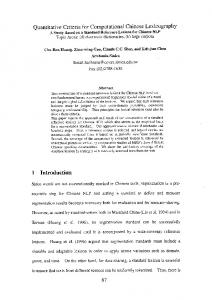
For this task, we train our classifier on 10,586 terms (9,451 terms in the training set and 1,135 in the development set), tune it on 4,435 terms, and evaluate it using 10,681 terms. The average F-score of the positive and negative classes for each dataset is given in the first part of Table 3. The best F-score value of 88.94 is achieved on the Twitter2013. We conducted an ablation study illustrated in the second part of Table 3 shows that all the selected features contribute well in our system performance. Other than the textual tokens feature, which refers to a bag of preprocessed tokens, the study highlights the role of the term polarity score feature: −4.20 in the F-score, when this feature is not considered on the TwitterSarcasm dataset. Another study conducted is a feature correlation analysis, in which we grouped features with similar intuitions. Namely the two features negative presence and negative words count are grouped as “negative features”, and the features positive 183
F-score Negative presence Positive words count Negative words count Polarity score Level of association Textual tokens
Twitter2014 TwitterSarcasm LiveJournal2014 Twitter2013 SMS2013 84.40 76.99 84.21 88.94 87.98 -0.45 0.00 -0.45 -0.23 +0.30 -0.52 -1.37 -0.11 -0.02 +0.38 -0.50 -2.20 -0.61 -0.47 -1.66 -1.83 -4.20 -0.23 -2.14 -3.00 -0.18 0.00 -0.18 -0.07 +0.57 -8.74 -2.40 -3.02 -4.37 -6.06
Table 3: Task-A feature ablation study. F-scores calculated on each set along with the effect when removing one feature at a time. Twitter2014 TwitterSarcasm LiveJournal2014 Twitter2013 SMS2013 F-score 84.40 76.99 84.21 88.94 87.98 Negative features -1.53 -0.84 -3.05 -1.88 -0.67 Negative presence -0.45 0.00 -0.45 -0.23 +0.3 Negative words count -0.50 -2.20 -0.61 -0.47 -1.66 Words count -1.07 -2.2 -0.79 -0.62 -2.01 Positive words count -0.52 -1.37 -0.11 -0.02 +0.38 Negative words count -0.50 -2.20 -0.61 -0.47 -1.66 Table 4: Task-A features correlation analysis. We grouped features with similar intuitions and we calculated F-scores on each set along with the effect when removing one feature at a time. 5% of the data). Hence the system could not learn from such a small set of neutral class examples. In the case of negative class error rate, 14.9%, most of which were classified as positive. An example of such classification: I knew it was too good to be true OTL. Since our system highly relies on lexicon, hence looking at lexicon assigned polarity to the phrase too good to be true which is positive, happens because the positive words good and true has dominating positive polarity. Lastly for the positive error rate, which is relatively lower, 6%, most of which were classified negative instead of positive. An example of such classification: Looks like we’re getting the heaviest snowfall in five years tomorrow. Awesome. I’ll never get tired of winter. Although the phrase carries a positive sentiment, the individual negative words of the phrase never and tired again dominates over the phrase.
fixed the size of our training dataset. Then, we compared the performance of our classifier using only the bag of tokens feature, in two different sizes. In the first experiment, we included all tokens collected from all tweets. In the second, we only considered the top 20 ranked tokens from each tweet. Tokens were ranked according to the difference between their highest level of association into one of the sentiments and the sum of the rest. The level of associations for tokens were determined using the Sentiment140 and SentiWordNet lexicons. The threshold number of tokens was identified empirically for best performance. We found that the classifier’s performance has been improved by 2 f-score points when the size of tokens bag is smaller. The experiment indicates that the contribution of the bag of words feature can be increased by reducing the size of vocabulary list.
6
Error Analysis
7
Our efforts are mostly tuned towards task-A, hence our inspection and analysis is focused on task-A. The error rate calculated per sentiment class: positive, negative and neutral are 6.8%, 14.9% and 93.8%, respectively. The highest error rate in the neutral class, 93.8%, is mainly due to the few neutral examples in the training data (only
Conclusion
We described our systems for Twitter Sentiment Analysis shared task. We participated in both tasks, but were mostly focused on task-A. Our hybrid system was assembled by integrating a rich set of lexical features into a framework of feature selection and parameter tuning, The polarity 184
F-score Negative presence Neutral words count Polarity score Sentiment frequency textual tokens
Twitter2014 TwitterSarcasm LiveJournal2014 Twitter2013 SMS2013 62.71 40.95 65.14 63.22 61.75 -1.65 +1.26 -3.37 -3.66 -0.95 +0.05 0.00 -0.72 -0.57 -0.54 -4.03 -6.92 -3.82 -3.83 -4.84 +0.10 0.00 +0.18 -0.12 -0.05 -17.91 +6.5 -21.07 -19.97 -15.8
Table 5: Task B feature ablation study. F-scores calculated on each set along with the effect when removing one feature at a time. score feature was the most important feature for our model in both tasks. The F-score results were consistent across all datasets, except the TwitterSarcasm dataset. It indicates that feature selection and parameter tuning steps were effective in generalizing the model to unseen data.
Saif Mohammad, Svetlana Kiritchenko, and Xiaodan Zhu. 2013. NRC-Canada: Building the State-ofthe-Art in Sentiment Analysis of Tweets. In Second Joint Conference on Lexical and Computational Semantics (*SEM), Volume 2: Proceedings of the Seventh International Workshop on Semantic Evaluation (SemEval 2013), pages 321–327, Atlanta, Georgia, USA.
Acknowledgment
Preslav Nakov, Sara Rosenthal, Zornitsa Kozareva, Veselin Stoyanov, Alan Ritter, and Theresa Wilson. 2013. SemEval-2013 Task 2: Sentiment Analysis in Twitter. In Second Joint Conference on Lexical and Computational Semantics (*SEM), Volume 2: Proceedings of the Seventh International Workshop on Semantic Evaluation (SemEval 2013), pages 312– 320, Atlanta, Georgia, USA.
We would like to thank Kemal Oflazer and also the shared task organizers for their support throughout this work.
References
Richard E. Neapolitan, 2014. Foundations of Algorithms, pages 257–262. Jones & Bartlett Learning.
Stefano Baccianella, Andrea Esuli, and Fabrizio Sebastiani. 2010. SentiWordNet 3.0: An Enhanced Lexical Resource for Sentiment Analysis and Opinion Mining. In Proceedings of the Seventh conference on International Language Resources and Evaluation (LREC’10), pages 2200–2204, Valletta, Malta.
Alexander Pak and Patrick Paroubek. 2010. Twitter Based System: Using Twitter for Disambiguating Sentiment Ambiguous Adjectives. In Proceedings of the 5th International Workshop on Semantic Evaluation, pages 436–439, Uppsala, Sweden.
Steven Bird, Ewan Klein, and Edward Loper. 2009. Natural Language Processing with Python. O’Reilly Media, Inc.
Bo Pang and Lillian Lee, 2008. Opinion Mining and Sentiment Analysis, volume 2, pages 1–135. Now Publishers Inc.
Chih-Chung Chang and Chih-Jen Lin. 2011. LIBSVM: A Library for Support Vector Machines. ACM Transactions on Intelligent Systems and Technology, 2:27:1–27:27.
Sara Rosenthal, Preslav Nakov, Alan Ritter, and Veselin Stoyanov. 2014. SemEval-2014 Task 9: Sentiment Analysis in Twitter. In Proceedings of the Eighth International Workshop on Semantic Evaluation (SemEval’14), Dublin, Ireland.
Dmitry Davidov, Oren Tsur, and Ari Rappoport. 2010. Enhanced sentiment learning using twitter hashtags and smileys. In Proceedings of the 23rd International Conference on Computational Linguistics: Posters, pages 241–249, Uppsala, Sweden.
Duyu Tang, Furu Wei, Nan Yang, Ming Zhou, Ting Liu, and Bing Qin. 2014. Learning SentimentSpecific Word Embedding for Twitter Sentiment Classification. In Proceedings of the 52nd Annual Meeting of the Association for Computational Linguistics, pages 1555–1565, Baltimore, Maryland.
Rong-En Fan, Kai-Wei Chang, Cho-Jui Hsieh, XiangRui Wang, and Chih-Jen Lin. 2008. Liblinear: A library for large linear classification. The Journal of Machine Learning Research, 9:1871–1874.
Theresa Wilson, Janyce Wiebe, and Paul Hoffmann. 2005. Recognizing Contextual Polarity in Phraselevel Sentiment Analysis. In Proceedings of the Human Language Technology Conference and Conference on Empirical Methods in Natural Language Processing, pages 347–354, Vancouver, B.C., Canada.
Minqing Hu and Bing Liu. 2004. Mining and Summarizing Customer Reviews. In Proceedings of the Tenth ACM SIGKDD International Conference on Knowledge Discovery and Data Mining, pages 168– 177, Seattle, WA, USA.
185