Oct 25, 2016 - We introduce co-occurring directions sketch- ing, a deterministic .... antees to (2) in spectral norm, but with a linear de- pendency of â on ε as in ...
Co-Occuring Directions Sketching for Approximate Matrix Multiply
arXiv:1610.07686v1 [cs.LG] 25 Oct 2016
Youssef Mroueh
Etienne Marcheret IBM T.J Watson Research Center
Abstract We introduce co-occurring directions sketching, a deterministic algorithm for approximate matrix product (AMM), in the streaming model. We show that co-occuring directions achieves a better error bound for AMM than other randomized and deterministic approaches for AMM. Co-occurring directions gives a (1 + ε)-approximation of the optimal low rank approximation of a matrix product. Empirically our algorithm outperforms competing methods for AMM, for a small sketch size. We validate empirically our theoretical findings and algorithms.
1
Introduction
The vast and continuously growing amount of multimodal content poses some challenges with respect to the collection and the mining of this data. Multimodal datasets are often viewed as multiple large matrices describing the same content with different modality representations (multiple views) such as images and their textual descriptions. The product of large multimodal matrices is of practical interest as it models the correlation between different modalities. Methods such as Partial Least Squares (PLS) [Weg00], Canonical Correlation Analysis (CCA)[Hot36], Spectral Co-Clustering [Dhi01], exploit the low rank structure of the correlation matrix to mine the hidden joint factors, by computing the truncated singular value decomposition of a matrix product. The data streaming paradigm assumes a single pass over the data and a small memory footprint, resulting in a space/accuracy tradeoff. Multimodal data can occupy a large amount of memory or may be generated sequentially, hence it is important for the streaming
Preliminary work. Under review by AISTATS 2017. Do not distribute.
Vaibhava Goel
model to capture the data correlation . Approximate Matrix Multiplication (AMM), is gaining an increasing interest in streaming applications (See the recent monograph [Woo14] for more details ). In AMM we are given matrices X,Y , with a large number of columns n, and the goal is to compute matrices BX , BY , with smaller number of columns ℓ, such that ||XY ⊤ − BX BY⊤ ||Z is small for some norm k.kZ . In streaming AMM, columns of BX , BY , need to be updated as the data arrives sequentially. We refer to BX and BY as sketches of X and Y . Randomized approaches for AMM were pioneered by the work of [DKM06]. The approach of [DKM06] is based on the sampling of ℓ columns of X and Y . [DKM06] shows that by choosing an appropriate sampling matrix Π ∈ Rn×ℓ , we obtain a Frobenius error guarantee (k.kZ = k.kF ):
XY ⊤ − XΠ(Y Π)⊤ ≤ ε kXk kY k , (1) F F F
for ℓ = Ω(1/ε2 ), with high probability. The same guarantee of Eq. (1) was achieved in [Sar06], by using a random projection Π ∈ Rn×ℓ that satisfies the guarantees of a Johnson- Lindenstrauss (JL) transform 2 2 (∀x ∈ Rn kΠxk ∼ (1 ± ε) kxk , with probability 1 − 2 δ), where ℓ = O(1/ε log(1/δ)). Other randomized approaches focused on error guarantees given in spectral norm (k.kZ = k.k) , such as JL embeddings or efficient subspace embeddings [Sar06, MZ11, ATKZ14, CNW15] that can be applied to any type of matrices X in input sparisty time [CW13]. [CNW15] showed that using a subspace embedding Π ∈ Rn×ℓ we have with a probability 1 − δ:
XY ⊤ − XΠ(Y Π)⊤ ≤ ε kXk kY k , (2) for ℓ = O((sr(X) + sr(Y ) + log(1/δ))/ε2 ), where kXk2
sr(X) = kXkF2 is the stable rank of X. Note that sr(X) ≤ rank(X), hence results stated in term of stable rank are sharper and more robust than the one stated with the rank [Sar06, MZ11, ATKZ14]. Covariance sketching refers to AMM for X = Y . An elegant deterministic approach for covariance sketching called frequent directions was introduced recently
Manuscript under review by AISTATS 2017
in [Lib13, GLPW15], drawing the connection between covariance matrix sketching, and the classic problem of estimation of frequent items [MG82]. Another approach for AMM, consists of concatenating matrices X and Y, and of applying a covariance sketch technique on the resulting matrix, this approach results in a looser guarantee; The right hand side in Equations (1),(2) is replaced by ε(kXk2F + kY k2F ). Based on this observation, [YLZ16] proposed to use the frequent directions algorithm of [Lib13] to perform AMM in a deterministic way, we refer to this approach as FDAMM. FD-AMM [YLZ16] outputs BX , BY such that
XY ⊤ − BX B ⊤ ≤ ε(kXk2 + kY k2 ), Y F F
(3)
for ℓ = ⌈ 1ε ⌉. The sketch length ℓ dependency on ε in randomized methods is quadratic, FD-AMM improves this dependency to linear. In this paper we introduce co-occuring directions, a deterministic algorithm for AMM. Our algorithm is inspired by frequent directions and enables similar guarantees to (2) in spectral norm, but with a linear dependency of ℓ on ε as in FD-AMM. Given with stable ranks, co-occuring p direction achieves the guarantee of (2) for ℓ = O( sr(X)sr(Y )/ε).
The paper is organized as follows: In Section 2 we review frequent directions, introduce our co-occuring directions sketching algorithm, and give error bounds analysis in AMM and in low rank approximation of a matrix product. We state our proofs in Section 3. In section 2.2.2 and Section 4 we discuss error bounds, space and time requirements, and compare our approach to related work on AMM and low rank approximation. Finally we validate the empirical performance of co-occuring directions in Section 5, on both synthetic and real world multimodal datasets. Notation. We note by C = U ΣV ⊤ , the thin svd of C, and by σmax (C) the maximum singular value, T r refers to the trace. σj are the singular values that are assumed to be given in decreasing order. Note that for C ∈ Rmx ×my the spectral norm is defined as follows kCk = maxu,v,kuk=kvk=1 u⊤ Cv = σmax (C). The nuclear norm (known also as trace or 1− schatten norm) kCk2
is defined as follows: kCk∗ = T r(Σ). sr(C) = kCkF2 is the stable rank of C. Assume C and D have the same number of column, [C; D] denotes their concatenation on their row dimensions. For n ∈ N, [n] = {1, . . . n}.
2
Sketching from Covariance to Correlation
In this section we review covariance sketching with the frequent directions algorithm of [Lib13] and state its
theoretical guarantees [Lib13, GLPW15]. We then introduce correlation sketching and present and analyze our co-occuring directions algorithm. 2.1
Covariance Sketching: Frequent Directions
Let X ∈ Rmx ×n , where n is the number of samples and mx the dimension. We assume that n > mx . The goal of covariance sketching is to find a small matrix DX ∈ Rmx ×ℓ , where ℓ max(mx , my ). Let BX ∈ R and BY ∈ Rmy ×ℓ (ℓ < n, ℓ ≤ min(mx , my )). Let η > 0 . The matrix pair (BX , BY ) is called an η-correlation sketch of (X, Y ) if it satisfies in spectral norm:
XY ⊤ − BX BY⊤ ≤ η.
Manuscript under review by AISTATS 2017
We now present our co-occuring directions algorithm (Algorithm 2). Intuitively Algorithm 2 sets a noise level using the median of the singular values of the correlation matrix of the sketch BX BY⊤ . The SVD of BX BY⊤ is computed efficiently in lines 8,9 and 10 of Algorithm 2 using QR decomposition. Left and right singular vectors below this noise threshold are replaced by fresh samples from X and Y , correlation sketches are updated and the process continues. Theorem 2 shows that our co-occuring directions algorithm outputs (BX , BY ) a correlation sketch of (X, Y ) as defined above in Definition 1. Algorithm 2 Co-occuring Directions 1: procedure Co-D(X ∈ Rmx ×n , Y ∈ Rmy ×n ) 2: BX ← 0 ∈ Rmx ×ℓ . 3: BY ← 0 ∈ Rmy ×ℓ . 4: for i ∈ [n] do 5: Insert a column Xi into a zero valued column of BX 6: Insert a column Yi into a zero valued column of BY 7: if BX , BY have no zero valued column then 8: [Qx , Rx ] ← QR(BX ) 9: [Qy , Ry ] ← QR(BY ) 10: [U, Σ, V ] ← SVD(Rx Ry⊤ ) 11: ⊲ Qx ∈ Rmx ×ℓ , Rx ∈ Rℓ×ℓ , my ×ℓ ℓ×ℓ ℓ×ℓ 12: ⊲ Qy ∈ R √, Ry ∈ R , U, Σ, V ∈ R . 13: Cx ← Qx U √ Σ 14: Cy ← Qy V Σ 15: ⊲ Cx , Cy not computed 16: δ ← σℓ/2 (Σ) ⊲ the median value of Σ ˜ ← max(Σ − δIℓ , 0) 17: Σ ⊲ shrinkage p ˜ 18: BX ← Q x U p Σ ˜ 19: BY ← Q y V Σ 20: ⊲ at least last ℓ/2 columns are zero 21: end if 22: end for 23: return BX , BY 24: end procedure
It is important to see that while frequent directions shrinks Σ2 , co-occuring directions filters Σ. We prove in the following an approximation bound in spectral norm for co-occurring directions. 2.2.1
Main Results
We give in the following our main results, on the approximation error of co-occurring direction in AMM (Theorem 2), and in the k−th rank approximation of a matrix product (Theorem 3). Proofs are given in Section 3.
Theorem 2 (AMM) The output of co-occuring directions (Algorithm 2) gives a correlation sketch (BX , BY ) of (X, Y ), for ℓ ≤ min(mx , my ) satisfying: For a correlation sketch of length ℓ, we have:
XY ⊤ − BX BY⊤ ≤ 2 kXkF kY kF . ℓ
2) Algorithm 2 runs in O(n(mx + my + ℓ)ℓ) time and requires a space of O((mx + my + ℓ)ℓ). Theorem 3 (Low Rank Product Approximation) Let (BX , BY ) be the output of Algorithm 2. Let k ≤ ℓ. Let Uk , Vk be the matrices whose columns are the k-th largest left and right singular vectors of BX BY⊤ . k ⊤ k ⊤ Let πU (X) = Uk U√ Let k X, πV (Y ) = Vk Vk Y . sr(X)sr(Y )
||X||||Y || we have: ε > 0, for ℓ ≥ 8 ε σk+1 (XY ⊤ )
XY ⊤ − π k (X)π k (Y )⊤ ≤ σk+1 (XY ⊤ )(1 + ε). U V
2.2.2
Discussion of Main Results
For ℓ = ⌈ 1ε ⌉, ε ∈ [ min(m1x ,my ) , 1] from Theorem 2 we see that (BX , BY ) produced by Algorithm 2 is an ηcorrelation sketch of (X, Y ) for η = 2ε kXkF kY kF . In AMM, bounds are usually stated in term of the product of spectral norms of X an Y as in Equation (2). Let kXk2F kXk2
be the stable rank of X. It is easy to see √ 2 sr(X)sr(Y ) , gives that co-occuring directions for ℓ = ε an error bound of ε kXk kY k. While in randomized √ methods the error is O(1/ ℓ), co-occuring direction’s error is O(1/ℓ). Moreover the dependency on stable p ranks in co-occuring directions is 2 sr(X)sr(Y ) ≤ sr(X) + sr(Y ), the lattter appears in subspace embedding based AMM [CNW15, MZ11, ATKZ14]. For X = Y co-occuring directions reduces to frequent directions of [Lib13], and Theorem 2 recovers Theorem 1 of [Lib13]. sr(X) =
Stronger bounds for frequent directions were given in [GLPW15] where the bound in Equation (4) is improved, for ℓ > 2k, for any k:
XX ⊤ − DX D⊤ ≤ X
2 2 kX − Xk kF , ℓ − 2k
where Xk is the k−th rank approximation of X (with X0 = 0). Hence by defining Z = [X; Y ] ∈ R(mx +my )×n and applying frequent directions to Z (FD-AMM [YLZ16]), we obtain BX , BY satisfying:
XY ⊤ − BX B ⊤ ≤ 2 kZ − Zk k2 , hence the perfoY F ℓ−2k mance of FD-AMM depends on the low rank structure of Z. A sharper analysis for co-occuring directions remains an open question, but the following discussion of Theorem 3 will shed some light on the advantages of co-occuring directions on FD-AMM [YLZ16].
Manuscript under review by AISTATS 2017
Theorem 3 shows that co-occuring directions sketching gives a (1 + ε)- approximation of the optimal low rank approximation of the matrix product XY ⊤ . Note that kXY ⊤ k σk+1 (XY ⊤ ) ≤ k+1 ∗ . Hence for ℓ ≥ 8(k + 1)/ε, we obtain a 1 + ε- approximation of the optimal k rank approximation of XY ⊤ . This highlights the relation between the sketch length in co-occurring directions ℓ and the rank of XY ⊤ . Note that the maximum rank of XY ⊤ is min(rank(X), rank(Y )). When using FD-AMM, based on the covariance sketch of the concatenation of X and Y , the sketch length ℓ is related to the rank of Z = [X; Y ]. Note that the maximum rank of the concatenation (Z) is bounded by rank(X) + rank(Y ). Hence we see that co-occuring directions guarantees a 1+ε approximation of the optimal k-rank approximation of XY ⊤ for a smaller sketch size then FD-AMM (min(rank(X), rank(Y )) for cooccuring directions versus rank(X) + rank(Y ) for FDAMM). In the following we comment on the running time of co-occuring directions. 2.2.3
Running Time Analysis and Parralelization.
Running Time. We compare the space and the running time of our sketch to to a naive implementation of the correlation sketch. 1) Naive Correlation Sketch: In the if statement of ⊤ Algorithm 2, compute p the ℓ thinpsvd SVD(BX BY ) = ˜ BY ← V Σ. ˜ We need a space [U, Σ, V ], BX ← U Σ, ⊤ O(mx my ) to store BX By . The running time is dominated by computing an ℓ thin svd O(mx my ℓ) each n ℓ/2 that is O(nmx my ), hence no gain with respect to brute force. 2) Co-occuring Directions: Algorithm 2 avoids computing BX BY⊤ by using the QR decomposition of BX and BY . The space needed is O(ℓ(mx + my + n , that is ℓ)). We have a computation done every ℓ/2 dominated by computing QR factorization and svd : O((mx + my + ℓ)ℓ2 ) (computing Rx Ry⊤ requires O(ℓ3 ) operations). This results in a total running time : O(n(mx + my + ℓ)ℓ). There is a computational and m m memory advantage when ℓ < mxx+myy . Parallelization of Co-occuring Directions (Sketches of Sketches). Similarly to the frequent directions [Lib13], co-occuring directions algorithm is simply parallelizable. Let X = [X1 , X2 ] ∈ Rmx ×(n1 +n2 ) , and Y = [Y1 , Y2 ] ∈ Rmx ×(n1 +n2 ) . Let 1 (BX , BY1 ) be the correlation sketch of (X1 , Y1 ), 2 and (BX , BY2 ) be the correlation sketch of (X2 , Y2 ). Then the correlation sketch (CX , CY ) 1 2 of ([BX , BX ], [BY1 , BY2 ]) is a correlation sketch of (X, Y ), and is as good as (BX , BY ) the correlation
sketch of (X, Y ). Hence we can sketch the data in M -independent chunks on M machines then merge by concatenating the sketches and performing another sketch on the concatenation, by doing so we divide the running time by M .
3
Proofs
In this Section we give proofs of our main results: Proof 1 (Proof of Theorem 2) By construction we have: � √ �� √ �⊤ Cx Cy⊤ = Qx U Σ Qy V Σ � ⊤ � ⊤ = Qx U ΣV ⊤ Q⊤ y = Qx Rx Ry Qy =
(Qx Rx ) (Qy Ry )⊤ .
Hence the algorithm is computing a form of R-SVD of BX BY⊤ , followed by a shrinkage of the correlation matrix. Let Bxi , Byi , Cxi , Cyi , Σi , Σ˜i , δi , the values ˜ δ after the execution of the of BX , BY , Cx , Cy , Σ, Σ, main loop. δi = 0 if we don’t enter the if statement (Bxi = Cxi and Byi = Cyi if we don’t enter the if statement). Hence we have at an iteration i: Cxi Cyi,⊤ = Bxi−1 Byi−1,⊤ + Xi Yi⊤ . Note that: XY ⊤ − BX BY⊤
= XY ⊤ − Bxn Byn,⊤ n X � Xi Yi⊤ + Bxi−1 Byi−1,⊤ − Bxi Byi,⊤ = i=1
=
n X i=1
� Cxi Cyi,⊤ − Bxi Byi,⊤ .
By the triangular inequality we can bound the spectral norm: n
i i,⊤
X
Cx Cy − Bxi Byi,⊤ .
XY ⊤ − BX BY⊤ ≤ i=1
We are left with bounding Cxi Cyi,⊤ − Bxi Byi,⊤ :
� i i i �⊤ �⊤ � ˜ Q V . Cxi Cyi,⊤ = Qix U i Σi Qiy V i , Bxi Byi,⊤ = Qix U i Σ y
Note that:
i i,⊤
Cx Cy − Bxi Byi,⊤
˜ i )(Qiy V i )⊤ = (Qix U i )(Σi − Σ
˜ i = Σi − Σ
≤ δi ,
where the first equality follows from the fact that, ˜ i is a diQix U i , Qiy V i , are orthonormal. And Σi − Σ agonal matrix with at least ℓ/2 entries equal δi or 0,
Manuscript under review by AISTATS 2017
and the other entries are less than δi . It follows that we have in spectral norm: n
X
XY ⊤ − BX BY⊤ ≤ δi . (5) Pn i=1 Now we want to relate i=1 δi to ℓ, and propreties of X, Y . Let k.k∗ , the 1− schatten norm. For a matrix A of P rank r, and singular values σi : kAk∗ = ri=1 σi (A). We have:
BX BY⊤ = Bxn Byn,⊤ ∗
∗
n X
i i,⊤
Bx By − Bxi−1 Byi−1,⊤ = ∗ ∗ i=1
n � X
i i,⊤
�
C C − B i−1 B i−1,⊤ = x y x y ∗ ∗ i=1
n � X
i i,⊤
�
Cx Cy − Bxi Byi,⊤ (6) − ∗ ∗ i=1
We have at an iteration i, the R-SVD of Cxi Cyi,⊤ and Bxi, Byi,⊤ :
i i,⊤
C C = T r(Σi ) and B i B i,⊤ = T r(Σ ˜ i ). x y x y ∗ ∗
Hence we by the definition
have
of the shrinking operation: Cxi Cyi,⊤ ∗ − Bxi Byi,⊤ ∗ =
˜ i) = T r(Σi − Σ X
=
δi +
ℓ X j=1
X
j,σji ≤δi
j,σji >δi
σji − σ ˜ji
σji ≥
ℓ δi . 2
(7)
where in the last inequality we used the CauchySchwarz inequality. Putting together Equations (5) and (10) we have finally:
XY ⊤ − BX BY⊤ ≤ 2 kXk kY k . (11) F F ℓ 2) Refer to Section 2.2.3. k Proof 2 (Proof of Theorem 3) Let πU (X) = ⊤ k ⊤ x Uk Uk X, πV (Y ) = Vk Vk Y . Let Hk be the span of x {u1 , . . . uk }, and Hm be the orthogonal of Hkx . Simx −k y y ilarly define Hk the span of {v1 , . . . vk }, and Hm y −k its orthogonal. For all u ∈ Rmx , kuk = 1, there exits ax , bx ∈ R, a2x + b2x = 1, such that u = ax wx + bx zx , x where wx ∈ Hkx , ||wx || = 1 and zx ∈ Hm , ||zx || = 1. x −k my Similarly for v ∈ R , kvk = 1 there exits ay , by ∈ R, a2y + b2y = 1, such that v = ay wy + by zy , where y wy ∈ Hky , ||wy || = 1 and zy ∈ Hm , ||vy || = 1 . y −k k Let ∆ = XY ⊤ − πU (X)πVk (Y )⊤ , we have k∆k = maxu∈Rmx ,v∈Rmy ,||u||=||v||=1 |u⊤ ∆v|
|u⊤ ∆v| = ≤ +
|(ax wx + bx zx )⊤ ∆(ay wy + by zy )| |ax ay ||wx⊤ ∆wy | + |bx by ||zx⊤ ∆zy |
|ax by ||wx⊤ ∆zy | + |bx ay ||zx⊤ ∆wy |
Since wx ∈ Hkx , wy ∈ Hky , we have wx⊤ ∆wy = 0. Since y x zx ∈ Hm , zy ∈ Hm , zx⊤ ∆zy = zx⊤ XY ⊤ zy . Simix −k y −k ⊤ ⊤ ⊤ larly wx ∆zy = wx XY zy , and zx⊤ ∆wy = zx⊤ XY ⊤ wy . Note that |ax |, |bx |, |ay |, |by | are bounded by 1. Hence we have (maximum is taken on each appropriate set defined above, all vectors are unit norm): max |u⊤ ∆v| ≤ u,v
max |zx⊤ XY ⊤ zy | + max |wx⊤ XY ⊤ zy |
zx ,zy
wx ,zy
On the other hand using the reverse triangle inequality + max |zx⊤ XY ⊤ wy | for the 1− shatten norm we have: zx ,wy
i i,⊤ i−1 i−1,⊤
y
Cx Cy − Bx By
≤ Cxi Cyi,⊤ − Bxi−1 Byi−1,⊤ For z ∈ Hx x ∗ ∗ ∗ mx −k , zy ∈ Hmy −k we have:
Recall that: Cxi Cyi,⊤ = Bxi−1 Byi−1,⊤ + Xi Yi⊤ , hence we |zx⊤ XY ⊤ zy | ≤ |zx⊤ (XY ⊤ − BX BY⊤ )zy | + |zx⊤ BX BY⊤ zy |
have: ≤ XY ⊤ − BX BY⊤ + σk+1 (BX BY⊤ )
i i,⊤ i−1 i−1,⊤
⊤
Cx Cy − Bx By
≤ Xi Yi = kXi k kYi k , 2 2 ∗ ∗ ∗ ≤ 2 XY ⊤ − BX BY⊤ + σk+1 (XY ⊤ ), (8) where we used that maxzx ∈Hxm −k ,zy ∈Hym −k |zx⊤ BX BY⊤ zy | since Xi Yi⊤ is rank one. Finally putting together Equax y tions (6), (7),(8), we have: = σk+1 (BX BY⊤ ) by definition of σk+1 . The n n last inequality follows from weyl inequality X X
ℓ
BX B ⊤ ≤ δi . (9) kXi k2 kYi k2 − |σk+1 (BX BY⊤ ) − σk+1 (XY ⊤ )| ≤ XY ⊤ − BX BY⊤ . Y ∗ 2 i=1
i=1
It follows from Equation (9) that: n X i=1
δi
n X
≤
2 ℓ
≤
v v u n u n X X u u 2 t 2 2 kXi k2 t kYi k2 ℓ i=1 i=1
=
i=1
kXi k2 kYi k2 − BX BY⊤ ∗
2 kXkF kY kF , ℓ
!
(10)
y Note that for wx ∈ Hkx and zy ∈ Hm we y −k have wx⊤ BX BY⊤ zy = 0. To see that, note that wx ∈ span{u1, . . . uk } , zy ∈ span{vk+1 , . . . vℓ }. Pℓ There exists βj , such that zy = j=k+1 βj vj , Pℓ Pℓ ⊤ hence BX BY⊤ zy = σ β u = i=1 j=k+1 i j i vi vj Pℓ j=k+1 σj βj uj ⊥ wx . Hence we have:
|wx⊤ XY ⊤ zy | =
≤
|wx⊤ (XY ⊤ − BX BY⊤ )zy |
XY ⊤ − BX B ⊤ . Y
Manuscript under review by AISTATS 2017 x Similarly for for zx ∈ Hm wy ∈ H ky we conx
−k and ⊤ ⊤ ⊤ clude that: |wx XY zy | ≤ XY − BX BY⊤ . Finally we have:
k∆k ≤ 4 XY ⊤ − BX BY⊤ + σk+1 (XY ⊤ )
where Ux ∈ Rn×kx , (Ux )i,j ∼ N (0, 1), Sx ∈ Rkx ×kx is a diagonal matrix with (Sx )jj = 1−(j −1)/kx , and Vx ∈ Rmx ×kx is such that Vx⊤ Vx = Ikx . Similarly we generate Y = Vy Sy Uy⊤ , Uy ∈ Rn×ky , Sy ∈ Rky ×ky , Vy ∈ Rmy ×ky . Hence X and Y are at most rank kx , and 8 kXkF kY kF ky respectively. We consider n = 10000, mx = 1000, ≤ + σk+1 (XY ⊤ ) my = 2000, and three regimes: both matrices have ℓ p a large rank (kx = 400, ky = 400), one matrix has a sr(X)sr(Y ) ||X||||Y || ≤ σk+1 (XY ⊤ )(1 + 8 ) ℓ σk+1 (XY ⊤ ) smaller rank then the other (kx = 400, ky = 40), and both matrices have a small rank (kx = 40, ky = 40). √ sr(X)sr(Y ) ||X||||Y || We compare the performance of co-occuring directions For ℓ ≥ 8 , we have: k∆k ≤ ε σk+1 (XY ⊤ ) to baselines given in Section 4 in those three regimes. σk+1 (XY ⊤ )(1 + ε). For randomized baselines we run each experiments 50 times and report mean and standard deviations of performances. Experiments were conducted on a single 4 Previous Work on Approximate core Intel Xeon CPU E5-2667, 3.30GHz, with 265 GB Matrix Multilply of RAM and 25.6 MB of cache. We list here a catalog of baselines for AMM: 60
Brute Force. We keep a running correlation C ← C + Xi Yi⊤ . We perform an ℓ thin svd at the end of the stream. Space O(mx my ), running time: O(nmx my ) + O(mx my ℓ), the cost of the sketch update and the ℓ thin svd. Sampling [DKM06]. We define a distribution over Pn ik , where S = i=1 kXi k kYi k. Form [n], pi = kXi kkY S BX and BY by taking ℓ iids samples (column indices), using pi . In the streaming model, since S is not known, we use ℓ independent reservoir samples. Hence the space needed is O(ℓ(mx + my )), the running time is O(ℓ(mx + my )n). Random Projection [Sar06]. BX , BY are of the n×ℓ form √ XΠ and , and Πij ∈ √ Y Π, where Π ∈ R {−1/ ℓ, 1/ ℓ}, uniformly. This is easily implemented in the streaming model and requires O(ℓ(mx + my )) space and O(ℓ(mx + my )n) time. Hashing [CW13]. Let h : [n] → [ℓ], and s : [n] → {−1, 1} be perfect hash functions. We initialize BX , BY to all zeros matrices. When processing columns of X and Y we update columns of BX and BY as follows: BX,h(i) ← BX,h(i) + s(i)Xi , BY,h(i) ← BY,h(i) +s(i)Yi . Hashing requires O(ℓ(mx +my )) space and O(n(mx + my )) time. FD-AMM [YLZ16]. Let Z = [X; Y ] ∈ R(mx +my)×n , let DZ be the output of frequent directions (Algoritm 1). We partition DZ = [BX ; BY ], and use BX and BY in AMM. This requires O(ℓ(mx + my )) space and O(n(mx + my )ℓ) time.
5
Experiments
AMM of Low Rank Matrices. We consider X ∈ Rmx ×n and Y ∈ Rmy ×n , generated using a non-noisy low rank model [GLPW15] as follows: X = Vx Sx Ux⊤ ,
50
Sampling Random Projection Hashing FD−AMM Co−Occ D. Brute Force
Time
40
30
20
10
0
0
100
200
300
400
500
600
700
800
900
1000
ℓ
Figure 1: Time given in seconds versus sketch length ℓ. We see in Figure 1, that hashing timing is, as expected, independent from the sketch length. Random projection requires the most amount of time. Cooccuring directions timing is on par with sampling and slightly better than FD-AMM. From Figure 2 1 we see that the deterministic baselines (a,c,e) consistently outperform the randomized baselines (b,d,f) in all three regimes. As discussed previously random√ ized methods error bound are of the order of O(1/ ℓ), while both co-occuring directions and FD-AMM have an error bound order O(1/ℓ). Note that the brute force error becomes zero (up to machine precision) when ℓ exceeds min(rank(X), rank(Y )). When comparing co-occuring direction to FD-AMM we see a clear phase transition for co-occuring direction as ℓ exceeds O(min(rank(X), rank(Y ))). For FD-AMM the phase transition happens when ℓ exceeds O(rank(X)+ rank(Y )). The phase transition happens earlier for cooccuring directions and hence co-occuring directions outperforms FD-AMM for a smaller sketch size. This is in line with our discussion in Section 2.2.2. For in1
Better seen in color.
Manuscript under review by AISTATS 2017
4
10 4
x 10
5
10 3
Sampling Random Projection Hashing
4.5
10 2
||X Y ⊤ − B X B Y⊤ ||
4
10 1
10 0
10 -1
10 -2
3.5
3
2.5
2
FD-AMM 10 -3
Co-Occ D. Brute Force
10 -4
10
1.5
1
-5
0.5 0
100
200
300
400
500
600
700
800
900
1000
0
200
400
600
800
1000
1200
ℓ
(a) no noise (kx = 400, ky = 400), error in log scale.
(b) no noise (kx = 400, ky = 400) error in linear scale. 4
10 4
10 3
Sampling Random Projection Hashing
2
||X Y ⊤ − B X B Y⊤ ||
10 2
10
x 10
2.5
FD-AMM Co-Occ D. Brute Force
1
10 0
10 -1
10 -2
1.5
1
10 -3
0.5 10 -4
10 -5
0 0
100
200
300
400
500
600
700
800
900
1000
0
200
400
600
800
1000
1200
ℓ
(c) no noise (kx = 400, ky = 40) error in log scale.
(d) no noise (kx = 400, ky = 40) error in linear scale. 10000
10 3
FD-AMM Co-Occ D. Brute Force
10 2
8000
||X Y ⊤ − B X B Y⊤ ||
10 1
10 0
10 -1
10 -2
10
-3
7000
6000
5000
4000
10 -4
3000
10 -5
2000
10
Sampling Random Projection Hashing
9000
-6
1000 0
100
200
300
400
500
600
700
800
900
1000
0
200
400
600
800
1000
1200
ℓ
(e) no noise (kx = 40, ky = 40) error in log scale.
(f) no noise (kx = 40, ky = 40) error in linear scale.
Figure 2: (a),(c),(e)Error of co-occuring directions versus the deterministic baseline FD-AMM, for clarity the error is given in log scale. (b)(d)(f) Error of co-occuring directions versus randomized baselines (sampling, random projection and hashing), for clarity the error is given in linear scale. stance plot (c) illustrates this effect, kx = 400, ky = 40, as ℓ exceeds 50, the error of co-occuring directions sharply decreases , while FD-AMM error is still high.
The latter starts a steep decreasing tendency when ℓ exceeds 400. We give plots for the low rank approximation as given in Theorem 3 for k = min(kx , ky ) in the
Manuscript under review by AISTATS 2017
appendix, we see a similar trend in the approximation error. AMM of Noisy Low Rank Matrices (Robustness). We consider the same model as before but we add a gaussian noise to the low rank matrices, i.e X = Vx Sx Ux⊤ + Nx /ζx , where ζx > 0, and Nx ∈ Rmx ×n , (Nx )i,j ∼ N (0, 1). Similarly for Y = Vy Sy Uy⊤ + Ny /ζy . In this scenario X and Y have still decaying singular values but with non zeros tails. We consider ζx = 1000, and ζy = 100. We compare here deterministic baselines in Figures 3,4, and 5, in the three scenarios we see that co-occuring directions still outperforms FDAMM, but the gap between the two approaches becomes smaller in the low rank regimes (Figures 4, and 5), this hints to a weakness in the shrinking of singular values in both algorithms getting affected by the noise (Step 17 in Alg. 2). We give plots for the low rank approximation in the appendix. 10
4
10
3
10
3
10
2
10
1
FD-AMM Co-Occ D. Brute Force
10 0
10
-1
10
-2
0
100
200
300
400
500
600
700
800
900
1000
Figure 5: Noisy (kx = 40, ky = 40). Error in log scale. ding HSKE of [MMG16] that results in a feature vector of dimension my = 3000. The training set size is n = 113287. We see in Fig. 6 that co-occuring directions outperforms FD-AMM in this case as well (timing experiment is given in the appendix). 10 0
FD-AMM Co-Occu D. Brute Force
10 2
10
10
-1
1
10 -2
10 0
10 -3
10
10
FD-AMM Co-Occ D. Brute Force
-1
10 -4
-2
0
100
200
300
400
500
600
700
800
900
1000
10 -5
10 -6
Figure 3: Noisy (kx = 400, ky = 400). log scale.
3
10
2
FD-AMM Co-Occ D. Brute Force
6
10 1
10
0
10 -1
10 -2
0
100
200
300
400
500
600
700
800
900
1000
Figure 4: Noisy(kx = 400, ky = 40). Error in log scale. Multimodal Data Experiments. In this section we study the empirical performance of co-occuring directions in approximating correlation between images and captions. We consider Microsoft COCO [LMB+ 14] dataset. For visual features we use the residual CNN Resnet101, [HZRS16]. The last layer of Resnet results in a feature vector of dimension mx = 2048. For text we use the Hierarchical Kernel Sentence Embed-
200
400
600
800
1000
1200
1400
1600
1800
2000
Figure 6: AMM error on MS-COCO.
10 4
10
0
Conclusion
In this paper we introduced a deterministic sketching algorithm for AMM that we termed co-occuring directions . We showed its error bounds (in spectral norm) for AMM and the low rank approximation of a product. We showed empirically that co-occuring directions outperforms deterministic and randomized baselines in the streaming model. Indeed co-occuring direction has the best error/space tradeoff among known baselines with errors given in spectral norm in the streaming model. We are left with two open questions. First, whether guarantees of Theorem 2 can be improved akin to the improved guarantees for frequent directions given [GLPW15]. This would give an explicit link of the sketch length ℓ, to the low rank structure of the matrix product XY ⊤ , and/or the low rank structure of the individual matrices. Second, whether robustness of co-occuring directions can be improved using
Manuscript under review by AISTATS 2017
robust shrinkage operators as in [GDP14].
References [ATKZ14] Michail Vlachos Anastasios T. Kyrillidis and Anastasios Zouzias. Approximate matrix multiplication with application to linear embeddings. In Corr, 2014. [CNW15]
Michael B. Cohen, Jelani Nelson, and David P. Woodruff. Optimal approximate matrix product in terms of stable rank. CoRR, 2015.
[CW13]
Kenneth L. Clarkson and David P. Woodruff. Low rank approximation and regression in input sparsity time. In STOC, 2013.
[Dhi01]
Inderjit S. Dhillon. Co-clustering documents and words using bipartite spectral graph partitioning. In KDD, 2001.
[DKM06]
Petros Drineas, Ravi Kannan, and Michael W. Mahoney. Fast monte carlo algorithms for matrices i: Approximating matrix multiplication. SIAM J. Comput., 2006.
[GDP14]
Mina Ghashami, Amey Desai, and Jeff M. Phillips. Improved Practical Matrix Sketching with Guarantees. 2014.
[GLPW15] Mina Ghashami, Edo Liberty, Jeff M. Phillips, and David P. Woodruff. Frequent directions : Simple and deterministic matrix sketching. CoRR, 2015. [Hot36]
Harold Hotteling. Relations between two sets of variates. Biometrika, 1936.
[HZRS16] Kaiming He, Xiangyu Zhang, Shaoqing Ren, and Jian Sun. Deep residual learning for image recognition. In CVPR, 2016. [Lib13]
Edo Liberty. Simple and deterministic matrix sketching. In KDD. ACM, 2013.
[LMB+ 14] Tsung-Yi Lin, Michael Maire, Serge J. Belongie, Lubomir D. Bourdev, Ross B. Girshick, James Hays, Pietro Perona, Deva Ramanan, Piotr Dollár, and C. Lawrence Zitnick. Microsoft COCO: common objects in context. EECV, 2014. [MG82]
J. Misra and David Gries. Finding repeated elements. Science of Computer Programming, 1982.
[MMG16] Youssef Mroueh, Etienne Marcheret, and Vaibhava Goel. Multimodal retrieval with asymmetrically weighted CCA and hierarchical kernel sentence embedding. ArXiv, 2016. [MZ11]
Avner Magen and Anastasios Zouzias. Low rank matrix-valued chernoff bounds and approximate matrix multiplication. In SODA, 2011.
[Sar06]
Tamas Sarlos. Improved approximation algorithms for large matrices via random projections. 2006.
[Weg00]
Jacob A. Wegelin. A survey of partial least squares (pls) methods, with emphasis on the two-block case. Technical report, 2000.
[Woo14]
David P. Woodruff. Sketching as a tool for numerical linear algebra. Found. Trends Theor. Comput. Sci., 2014.
[YLZ16]
Qiaomin Ye, Luo Luo, and Zhihua Zhang. Frequent direction algorithms for approximate matrix multiplication with applications in CCA. In IJCAI, 2016.
Manuscript under review by AISTATS 2017
A
Low Rank product Approximation 10 4
10 0
FD-AMM Co-Occ D.
FD-AMM 10 3
Co-Occ D. 10 -1
10 2
10 1 10 -2 10 0
10 -1 10 -3
10
-2
10 -3
0
100
200
300
400
500
600
700
800
900
1000
10 -4
0
100
(a) (kx = 400, ky = 40) error in log scale.
200
300
400
500
600
700
800
900
1000
(b) (kx = 40, ky = 40) error in log scale.
Figure 7: No noise : Low rank approximation of matrix product, after projection on left and right singular vectors of BX BY⊤ for k = min(kx , ky ) = 40.
10 4
10 3
FD-AMM Co-Occ D.
FD-AMM Co-Occ D.
10 3
10 2
10 2
10 1
10 1
0
100
200
300
400
500
600
700
800
900
1000
(a) (kx = 400, ky = 40) error in log scale.
10 0
0
100
200
300
400
500
600
700
800
900
1000
(b) (kx = 40, ky = 40) error in log scale.
Figure 8: Noisy : Low rank approximation of matrix product, after projection on left and right singular vectors of BX BY⊤ for k = min(kx , ky ) = 40.
B
MS-Coco Timing Experiments
Manuscript under review by AISTATS 2017
2000
1800
1600
1400
Time
1200
1000
800
600
FD-AMM Co-Occ D. Brute Force
400
200
0 0
200
400
600
800
1000
1200
1400
1600
1800
2000
Figure 9: Timing of sketching on MS-COCO.