Representation learning, Deep Neural Network, Pairwise Constraint,. Metric Learning ... applications such as structured feature embedding[24] and face recognition[27]. ...... 2016. Deep metric learning via lifted structured feature embedding.
Co-Representation Learning For Classification and Novel Class Detection via Deep Networks Anonymous Author(s) ABSTRACT Deep Neural Network (DNN) has been largely demonstrated to be effective for closed-world classification problems where the total number of classes are known in advance. However, when the total number of classes that may occur during test time is unknown, DNNs notorious fail, i.e., DNN will make incorrect label prediction on instances from novel or unseen classes. This severely limits its utility in many real-world web applications, particularly when data occurs as a continuous stream. In this paper, we focus on addressing this key challenge by developing a two-channel DNN based co-representation learning framework that not only predicts instances from known classes, but also detects and adapts to the occurrence of novel class instances over time. Concretely, we propose a metric learning method using pairwise-constraint loss (PCL) function to learn a feature representation where intra-class compactness and inter-class separation is achieved. Moreover, we apply the temperature scaling scheme on the softmax function to replace traditional softmax output and design an open-world classifier. Our extensive empirical evaluation on benchmark datasets demonstrates the effectiveness of our framework compared to other competing techniques.
KEYWORDS Representation learning, Deep Neural Network, Pairwise Constraint, Metric Learning, Novel Class Detection
1
INTRODUCTION
Studies in recent years employing Deep Neural Networks (DNNs) has high performance in the classification task, which has lead to significant progress in a variety of real-world applications such as image classification[9, 11] and segmentation recognition[8]. However, one of the known shortcomings of DNN is that it can be overly confident[10, 23] when presented with classes which were not present in the training set. A DNN would incorrectly predict the label of instances from new (unknown) classes as one belonging to a known class with high confidence, especially when such instances share some resemblance to the training set instances. Therefore, it is crucial to design a DNN model that expects arrival of instance belonging to novel class during test time. Being able to accurately detect novel class examples is important for reducing classification errors and may also serve as the first step to build lifelong learning systems[14]. Permission to make digital or hard copies of part or all of this work for personal or classroom use is granted without fee provided that copies are not made or distributed for profit or commercial advantage and that copies bear this notice and the full citation on the first page. Copyrights for third-party components of this work must be honored. For all other uses, contact the owner/author(s). Conference’17, July 2017, Washington, DC, USA © 2018 Copyright held by the owner/author(s). ACM ISBN 978-x-xxxx-xxxx-x/YY/MM. https://doi.org/10.1145/nnnnnnn.nnnnnnn
Novel/Unseen class can be observed in various web applications such as the emergence of new topics in online news report, and occurrence of new categories of fashion images shared on social network platforms e.g., Instagram. Therefore, it is imperative to detect such novel-class instances along the data stream for a superior prediction performance. One-class SVM[28] is the earliest approach to addressing the challenge of novel-class detection. Moreover, recent studies [6, 7, 19, 21] have proposed solutions to further improve one-class SVM. Particularly, these methods are based on an assumption that instances belonging to the same class tend to occur close to each other in its feature space, (called cohesion), compared to instances associated with different class labels (called separation). Unfortunately, these properties are not intrinsically observed in many real-world high dimensional scenario, particularly in computer vision applications such as traffic signs recognition, and outdoor scene recognition system in the self-driving cars. Here, the inter-class distances maybe even smaller than intra-class distances if images from different classes share some visual properties. More recently, studies addressing the open-world classification problem over DNNs have proposed various changes at the output layer or pre-processing. For example, [1, 10] aims to assign higher softmax/open-max scores to the examples from the training set, while [26] proposes to replace the softmax layer with a 1-vs-rest layer consist of sigmoid activation functions. On the other hand, studies such as [3, 18] focus on the input pre-processing, which introduces small perturbations for the input examples. These techniques only utilize class labels available in the training data while ignoring the similarity or dissimilarity constraints among inter-class and intra-class sample pairs, though these constraints have been shown to provide superior information for feature representation learning [17]. Such feature representation may provide distinguishable features suitable for novel class detection. In the paper, we aim to compute a feature representation for novel class detection by exploring pairwise loss between inter-class and intra-class sample pairs, to be added to the output layer of a DNN. The pairwise loss could be regarded as a constraint for finding a suitable feature representation, which is used to improve the performance of classification and novel detection. Pairwise constraint between examples are commonly applied to learn a distance metric[31] in applications such as large-scale image recognition [13, 20, 29]. It utilizes similar pairs and dissimilar pairs as input, with a goal of generating a distance-metric that minimizes the distance between similar examples, and maximizes that between dissimilar samples. [5] proposed a Siamese network with a contrastive loss for image recognition, and has been applied to many real-world applications such as structured feature embedding[24] and face recognition[27]. Furthermore, studies [2, 25] have also explored computing feature representations using triplet-loss where constraints are specified by relative similarity and dissimilarity among instances. Unlike these studies, we aim to combine the constraint
loss and label information to improve feature representation for both novel class detection and open-world classification tasks. Concretely, our co-representation learning framework with metric learning mechanism aims to learn a feature representation where samples from the same class form clusters in embedded space, while being well separated from clusters of other classes. We call this framework RLCN. The key idea is to construct a DNN [11] structure with a pairwise constraint loss (PCL) function to improve the intra-class compactness and inter-class separateness, making the novel class detection more practical. We implement the framework by jointly training of the PCL and classification loss function on the top layer of DNN. Specifically, we apply the temperature scaling scheme[12] over the softmax output, and design an Open-World Classifier (OWC) to predict among existing class instances while detecting novel class instances simultaneously. The contributions of this paper are as follows. (1). We propose a co-representation learning framework with a pairwise constraint loss function to learn a high-level feature representation suitable for both classification and detection task. (2). We design an adaptive threshold detection method under the temperature scaling softmax probability, which is more appropriate for novel class detection. (3). We empirically evaluate our framework on real-world image and text dataset to comprehensively evaluate the performance of our proposed framework. The rest of this paper is organized as follows. We first illustrate our proposed approach in Section 3, and discuss our method’s complexity in Section 4. Next, we present the results of our empirical evaluation in Section 5, and finally conclude in Section 6.
2
Open-World Classifier
Pairwise Constrain Loss Classification Loss
2
f
(Xi , Xj )
Classification Loss
Embedding Layer
h
(2)
W
Hidden Layer
h
(2)
(1)
W
(1)
Share Weight Input Layer Xi
Xj
Figure 1: Overview of the RLCN framework.
3.1
Metric Learning with Pairwise Constrain
The relationships between sample pairs is used to generate the distance metric. Here we define a small set of M constraints between points x i , x j ∈ D, denoted as M = {(x i , x j , Si j )} where i, j ∈ {1...m} are the indices of the two points of the constraint, and Si, j ∈ {−1, 1} indicates whether the points are similar or not. The representations ϕ of instances x i and x j is calculated by passing them to multiple layers of nonlinear transformations. The intuition of using a DNN is as follows. Assume that there are N layers in our network. For the example x ∈ R d , the output of the first layer should be h (1) (x) = σ (W (1)x + b (1) ), where W (1) is a projection matrix to be learned in the first layer, b (1) is a bias vector and σ is a nonlinear activation function. Final representation ϕ(x) with N hidden layers can be computed as:
PROBLEM SETTING
m , where x ∈ R d is a Given a training dataset D = {(x i , yi )}i=1 i training instance and yi ∈ Y = {1, 2, . . . , k } is the associated class label, and a testing data set S = {(x t , yt )}tn=1 (n > m), where x t ∈ R d and yt ∈ Y ′ = {1, 2, . . . , k, k + 1, . . . , k ′ } (k ′ > k), the problem of classification is to predict the class label yˆt ∈ Y ′ for each x t ∈ S at time t. The problem of novel class is envisioned as follows: Let a classifier f be trained on dataset D, which is then used to predict the instances x t ∈ S. When the f could not able to determine whether x t belongs to a known class in Y , then x t could be judged as an novel class instance. Note that for any two arbitrary classes ya , yb ∈ Y ′ (ya , yb ), there are two instances x i and x j have the correspond class ya , and one instance x k associates with class yb , it is possible that ||x i − x k ||2 < ||x i − x j ||2 .
3
d
ϕ(x) = h (N ) (x) = σ (W (N )h (N −1) + b (N ) ), where h (n) = σ (W (n)h (n−1) + b (n) ), ∀n = 1, . . . , N ; h (0) = x . (1) Given x i and x j ∈ R d , they can be finally represented as ϕ(x i ) and ϕ(x j ). Their final level representations’ distance can be measured by computing the squared Euclidean distance as D ϕ2 (x i , x j ) =
THE RLCN FRAMEWORK
||ϕ(x i ) − ϕ(x j )||22 . In order to handle the problem setting, we proposed PCL, which is used to map similar (Si, j = 1) input instances together so that their distance would be smaller than a pre-specified margin value τ with a constant range value γ , and dissimilar (Si, j = −1) pairs should larger than margin with γ in the output representation space. We use the following constrained function to describe the relationship between D ϕ2 (x i , x j ), margin value τ and constant range value γ :
The goal of the RLCN is generating a proper feature representation ϕ to address classification and novel class detection simultaneously. Here, as shown in Figure 1, we first introduce the proposed pairwise constraint loss (PCL) for metric learning, and perform a comparison between our method and the commonly used loss function (like contrastive). Next, the co-representation learning of PCL and one-vs-rest classification loss is introduced, following with the discussion of why it is appropriate for classification and novel class detection. And the design of Open-World Classifier is provided at the end of this section. Algorithm 1 illustrates the details of classification and novel class detection process in RLCN.
Si, j (τ − D ϕ2 (x i , x j )) > γ 2
(2)
seek for the optimal value of ϕ: arg min LPC = Lpair + Lr eдul ar izat ion
Previous Metric Learning method
ϕ
τ
=
τ
M N 1 Õ λ Õ (||W (l ) ||F2 ) д(γ − Si, j (τ − D ϕ2 (x i , x j ))) + 2 i, j=1 2M l =1
Class 1
(4)
Class 2
Before
After
where l is the number of layers in the network structure, ||W ||F represents the Frobenius norm of the weightW , λ is a regularization parameter.
(a)
Pairwise Constrain Metric Learning
3.2 γ
In contrast to traditional multi-class classifiers that typically use softmax as the final layer, inspired by [26], we apply a one-vs-rest binary classification loss at the final output layer. It contains m sigmoid functions for m seen/existed classes. For the mth sigmoid function corresponding to label Ym , classification layer takes all examples with label y = Ym as positive examples and the rest with y , Ym as negative examples. Let Lcl assif y denote the loss introduced by the binary classification error (BCE). Formally, the classification loss is the following:
τ
Class 1 Class 2
Before
Co-Representation Learning
γ
After
(b)
Figure 2: Comparison between our proposed pairwise constrain loss and the previous loss (contrastive) function. (a) Shows the results after the mapping with contrastive loss. (b) Shows the results after the mapping using the PCL.
Lcl assif y = − Here 0 < γ < τ , the Eq. 2 could also be written as: 1−S τ +D ϕ2 (x i , x j )} + 2 i, j
S i, j +1 2
max{0, γ −
M 1 Õ д(γ − Si, j (τ − D ϕ2 (x i , x j ))) 2 i, j=1
[
K Õ
x i ,yi ∈D m=1
I(yi = Ym ) log дYm (x i )
+ I(yi , Ym ) log(1 − дYm (x i ))], 1 where дYm (x i ) = 1 + exp (−Wm⊤ (x i ))
max{0, γ +τ −D ϕ2 (x i , x j )}. Comparing with
previous loss function (contrastive loss) designed for metric learning method used in DNN like [5, 24], our method would be more flexible in practice. As shown in Fig. 2, in the original feature space, the distance between the samples in the same class may larger than the distance from different classes, after mapping with our PCL, the distance between similar pairs will be smaller than a margin minus a small range τ − γ , and the distance between dissimilar pairs will be larger than τ + γ . For previous contrastive loss, which penalizes the intra-class distance to zeros and the inter-class distances bigger than a fixed positive margin. For it’s object function: S i, j 1+S i, j 2 2 2 max{0, D ϕ (x i , x j )} + 2 max{0, m − D ϕ (x i , x j )}, we could regard it as a special case of PCL when τ = γ ( then m = τ + γ , m is the margin of the contrastive). Under this situation, the distance between similar pairs may be limited to be zero, so it’s constraint may be too strong and thus may not be suitable for the real-world scenario. The final constrained pairwise function is described as the following: Lpair =
Õ
(5) Here I is the indicator function, and Wm describes the weight of mth class in the final layer, we joint training Eq.3 and Eq.5 in our two-channel DNN structure. The overall objective function of previous tasks is now denoted as L: arg min L = Lcl assif y + α LPC . ϕ
(6)
Discussion Here α is a hyper-parameter that controls the importance of PCL in L. The PCL can be viewed as a regularization constraint on the feature representation, it pulls the samples closer to their corresponding classes, and make the features within the same class more compact, so it is beneficial for the classification. Through co/joint training pairwise loss and one-vs-rest classification loss, the framework can learn an intra-class compact and inter-class separable feature representation, which is appropriate for the novel class detection task.
(3)
3.3
Open-World Classifier (OWC)
Prior works have established the use of temperature scaling (or distillation) in DNN[12], further more, [4] calibrate the prediction confidence of the scaled softmax output. So the framework would apply distilled softmax probability to estimate the prediction label and do further open-world classification. We denote fi (x t ; ϕ), i ∈ {1, 2, . . . , k } as the final layer’s output for the i th class in Y under feature representation ϕ. For every instance x t ,
where M is the number of pairs used for training, we use д(x) = 1 log(1 + exp(βx)), which is a generalized logistic loss function, β and used as an approximation of hinge loss h(x) = max(x, 0) [20]. β could be regard as a sharpness parameter. In order to avoid overfitting, we add an frobenius regularization term to Eq. 3. We could minimize the PCL through Stochastic Gradient Descent (SGD) to 3
Algorithm 1 RLCN
RLCN would compute the temperature scaling softmax probability Si (x t ;T ) for class Yi : exp (fi (x t ; ϕ)/T ) Si (x t ;T ) = Í k exp (f (x ; ϕ)/T ) j t j=1
Require: S - Test data; M - The maximum size of generated constrain pairs in D; D - Initial training data in warm-up phase; E - epoch number for training the network; E - learning rate Ensure: Label y˜ predicted on S data. 1: Generate M sample pairs from D as describe in Sec. 3.1 2: // Training: 3: for every epoch E: do 4: random select a sample pair (x i , x j , Si j ) in M 5: do forward propagation to get representation ϕ(x i ), ϕ(x j )
(7)
where T ∈ R + is the temperature scaling parameter. A good manipulation of T’s value can push the softmax probability of different classes further apart from each other, and for x t ∈ S, we would get the maximum softmax probability Syˆ (x t ;T ) = argmaxi Si (x t ;T ) with it’s correspond label Yi , then compared it with threshold to determine whether x t belongs to novel class. Here a suitable and adaptive threshold value should be generated automatically for novel class detection, a common method is to apply the average prediction probability of training data for confidence threshold, for every class Yi , we have: Õ 1 Si (x;T ) (8) S¯i = ||D i ||
update W for classification loss in Eq. 5 : ∇W1 =
7:
∂ Lcl as s i f y ∇W2 = ∂W2 W1 = W1 − E∇W1 , W2 = W2 − E∇W2 ∂ LP C ∂ LP C , ∇ϕ(x j ) = ∂ϕ(x ∇ϕ(x i ) = ∂ϕ(x i) j)
8: 9: 10: 11:
x ∈D i
12:
where D i = {(x, y = Yi ), ∀x ∈ D}, i ∈ {1, 2, . . . , k}. ||D i || means total account of instance in D i ,S¯i has a t distribution with d f = ||D i || − 1 degrees of freedom. The desired Tnovel for class Yi is the 100(1 − α)% confidence lower bound of S¯i is given by p Tnovel (Yi ) = S¯i − t α,d f SDYi / ||D i || (9)
13: 14:
∂ Lcl as s i f y ∂W1
,
update ϕ for PCL: ϕ = ϕ − E(∇ϕ(x i ) + ∇ϕ(x j )) end for // Testing: repeat Receive a new instance x t from S. Predict label yˆ for x t using Eq. 7 and make prediction yˆ = argmax Si (x t ;T ) i ∈Y
15: 16:
where SDYi is the sample standard deviation of {Si (x;T ), ∀x ∈ Di }. Once we have the threshold Tnovel , classification and novel class detection is trivial. For the instance x t ∈ S, we check if the output maximum softmax probability Syˆ (x t ;T ) is less than the correspond class’s threshold Tnovel (Yi ) . If so, x t is a candidate from a novel class, and the predicted class for x t would be y˜ = −1; else, y˜ = argmax Si (x t ;T ). We evaluate the performance of our
17: 18: 19: 20:
if yˆ = −1 then Detect x t as Novel Class. else y˜ ← yˆ end if until S exists
a set of natural color images of 32x32 pixels, it contains 10 classes, 60,000 instances overall. SVHN4 contains 32x32 images with 3 color channels. Many images may contain multiple numbers but only assign one of them as the class. For all the image dataset, the preprocessing of the instances is a global normalization that normalizes the pixel values of the image to 0-1. In addition, we use one real news text dataset, which is from New York Times crawled through their public API5 . We obtain articles in 20 categories from Jan.1, 2006 to Jan.1, 2018. Each item is preprocessed via the word2vec technique6 to produce a 300dimension feature vector. For the classification task, we randomly select different numbers (200, 500 and 1000 samples for each class) of training samples from the training set includes all the classes. For the novel class detection task, we hold out some classes (as novel classes) in training and mix them back during testing. We choose 50% classes for the training step and all classes for testing. Taking MNIST as an example, for 50% classes, we randomly select 5 classes from the whole label set (totally 10 classes) 10 times and average the results.
i ∈Y
framework using various metrics in the experiment section.
4
6:
TIME AND SPACE COMPLEXITY
Overall, the execution overhead of RLCN mainly arises from the metric training, since we use SGD (Stochastic Gradient Descent) to optimize the gradient, the time complexity of calculating the gradient of one example is a constant C. With the mini-batch size Tmini and epoch number ne , time complexity of RLCN should be: 2 C). In our implementation, we use a GPU for computaO(ne Tmini tional acceleration (GTX 960 4GB). The space complexity of RLCN is O(TD + Bspace ), where TD represents the size for training dataset D, and Bspace represents the space complexity of the classifier utilized in the framework respectively.
5 EMPIRICAL EVALUATION 5.1 Dataset We use four publicly available benchmark real-world image datasets including FASHION-MNIST [30], MNIST [16], CIFAR-10 [15] and SVHN [22] for evaluation. The MNIST1 dataset contains 70, 000 images of handwritten digits. FASHION-MNIST2 dataset is designed as a difficult drop-in replacement for MNIST. CIFAR-103 is
We compare RLCN with competing state-of-the-art methods for both classification and novel class detection task: (1) One-class
1 http://yann.lecun.com/exdb/mnist/
4 http://ufldl.stanford.edu/housenumbers/
2 https://github.com/zalandoresearch/fashion-mnist
5 http://developer.nytimes.com/
3 https://www.cs.toronto.edu/
5.2
Baselines
6 https://radimrehurek.com/gensim/index.html
kriz/cifar.html 4
10000 5000 2000 Accuracy (%) Accuracy (%) Accuracy (%) DOC 90.27 ±0.22 72.89 ±0.21 25.72 ±0.21 DNN-hen 97.19±0.08 96.45±0.13 94.89±0.18 RLCN-CL 97.82±0.12 97.24±0.15 95.88±0.17 RLCN 98.54±0.11 97.96±0.14 96.52±0.18 Table 1: Classification performance on MNIST dataset corresponding to different amounts of training samples. Methods
Figure 3: Visualization of feature representation of existed/known and novel classes from MNIST dataset, the left one is the two types of classes in original representation, right one is processed through RLCN.
SVM (only detection): baseline classifier for novel detection; (2) ECSMiner (only detection) [19]: an ensemble framework to detect novel classes using K-Means clustering; (3) ECHO-D (only detection) [7]: an improved framework of ECSMiner through training on dynamically-determined chunks of data; (4) SENC-MaS (only detection) [21]: a framework that maintains two low-dimensional sketches of data representation to detect novel classes; (5) DOC (both)[26]: DNN model with one-vs-rest final sigmoid layer for classification and detection; (6) DNN-hen (both)[10]:common DNN model apply softmax function in the final layer; and (7)RLCN-CL (both): a modification of our framework that replace pairwise loss with contrastive loss;
5.3
class and the rest of them are regarded as the novel class. We first train the RLCN on the known class of MNIST set, then we feed the test data from both known and novel classes to the trained framework and obtain their feature representations, the results are shown in Fig.3. The Visualization of different result from MNIST indicates that compared with original feature space, the learned representations for known classes are intra-class compact and inter-class separable, so the novel class is distinguishable and the detection task would be appropriated. Classification performance: We conduct 10 independent experiments with different amounts of training samples on each dataset. Here, due to the limitation of the required pages, we only show the mean and standard deviation of performance of MNIST in Table 1. As we observe that our framework outperforms other state-of-art methods with different amounts of training samples. Comparing the accuracy between RLCN and DOC, DNN-hen, it is obvious that the PCL helps to improve the performance of the classification, particularly when the number of training instances is small (such as 2000 for all classes). It means when the information directly comes from the label is limited, pairwise constraints could provide extra information to learn a better feature representation, so that better classification performance is observed. Finally, the result between RLCN and RLCN-CL proves that our PCL outperforms the contrastive loss as described in Sec. 3.1. Similar results could be observed in other datasets, which indicate RLCN could maintain high performance for the classification work. Evaluation For Novel Class Detection On All Datasets: Table 2 compares novel class detection performance of RLCN with all baseline methods on each dataset. We observe that both ECSMiner and ECHO fails to detect any novel class on most complexity feature representation. On the other hand, SENC-MaS could detect some concept evolution instances with poor precision while missing most of such instances. The previous result shows that the strong global cohesion and separation assumption is invalid for many web application high dimensional datasets. For the DNN-based models, they show much more efficient result compared with previous traditional model, however, the results from DNN with multiple loss constrain (RLCN-CL, RLCN) are better than the DNN with single loss function (DOC, DNN-hen). It proved that adding constrain loss helps to improve the quality of the feature representation, and relax the assumption about cohesion and separation. So that RLCN-CL
Experiment Setup
We implement RLCN using Pytorch 0.4.0 library7 , and the deep neural network is the LeNet-5 which consists of 2 convolutional layers and n = 2 fully connected layers. The training step consists of 50 epochs, the learning rate is 0.01, and mini-batches size is 64. All baseline methods are based on code released by corresponding authors, except SENC-MaS. Due to unavailability of a fully functional code of SENC-MaS, we use our own implementation based on the author’s description. Hyper-parameters of these baseline approaches were set based on values reported by the authors. In RLCN, we set τ = 3 and γ = 1 for the margin value of the PCL, and T = 6 for the distillation softmax probability.
5.4
Evaluation Metrics
Let F N be the total novel class instances misclassified as existing class, F P be the total existing class instances misclassified as novel class, Nc be the total novel class instances in the test set, and N be the total number of instances in the test set. We use the following metrics to evaluate our approach and compare it with baseline known methods. (a) Accuracy%: Anew +A , where Anew is total number m of novel class instances classified correctly, Aknown is the number of known class instances identified correctly, and m is the total number of instances in the test set. (b) M new : % of novel class instances misclassified as existing class, i.e. F NN∗100 . (c) F new : % of c ∗100 . existing class instances misclassified as novel class, i.e. FNP−N c
5.5
Results
Performance of feature representation: We conduct experiments on MNIST dataset to demonstrate the effectiveness of representation learning of RLCN and used for novel class detection. We random select 50% of the whole MNIST classes as the known/existed 7 https://pytorch.org/
5
Methods One-Class SVM ECSMiner SENC-MaS ECHO-D DOC DNN-hen RLCN-CL RLCN
FASHION-MNIST M new F new 85.84±0.18 4.89±0.11 88.72±0.24 89.76±0.10 5.36±0.13 83.19±0.64 62.18±0.25 63.73±0.16 51.04±0.25 49.82±0.22
2.95±0.06 3.12±0.04 2.64±0.03 2.17±0.03
MNIST M new F new 63.07±0.08 2.33±0.02 67.11±0.24 2.49±0.02 78.56±0.34 4.94±0.46 60.42 ±0.18 2.76±0.28
CIFAR-10 M new F new 100.00±0.00 100.00±0.00 95.61±0.04 6.80±0.06 100.00±0.00 -
SVHN M new F new 100.00±0.00 100.00±0.00 98.51±0.13 5.22±0.07 100.00±0.00 -
42.08±0.10 41.95±0.08 29.65±0.18 29.94±0.16
63.71±0.27 64.33±0.21 58.81±0.20 55.09±0.15
61.17±0.24 63.09±0.18 55.07±0.18 53.14±0.25
1.90±0.09 1.88±0.11 1.48±0.11 1.40±0.12
4.91±0.14 5.17±0.15 3.85±0.11 3.93±0.12
5.01±0.15 5.25±0.21 3.87±0.18 3.34±0.16
New-York-Times M new F new 97.25±0.15 4.91±0.17 96.52±0.16 4.82±0.22 96.31±0.05 7.54±0.06 97.08±0.14 5.07±0.11 58.41±0.22 59.03±0.25 57.27±0.21 56.49±0.24
4.15±0.14 4.21±0.16 3.38±0.15 3.29±0.16
Table 2: Novel class detection performance over all datasets. Here - denotes failure of novel class detection.
(a)
(b)
Figure 5: ROC curves of other baselines and RLCN (purple line) on fashion-mnist dataset (c)
(d)
we observe that increasing the value of T in a certain range can improve the detection performance, however, the effects diminish when T is larger than a constant value (most often when T = 10). Thus, in general, it is suggested to start with τ = 3 and T = 6 for any given dataset.
Figure 4: Parameter sensitivity (τ and T ) for all datasets.
and RLCN could provide the lower M new value compared to other DNN baselines. What’s more, compared to the modification version RLCN-CL, the result shows that RLCN has better values in the most dataset, it demonstrates that the pairwise constrain from RLCN is more suitable for novel detection. What’s more, from Figure 5 which describes the ROC curves of other methods and RLCN (purple) on FASHION-MNIST dataset. We observe a strikingly increasing gap between RLCN and other baselines especially the common DNN model[10]. So it is appreciate for RLCN to execute novel class detection task. Parameter Selection: The two main parameters in RLCN is the margin value τ for PCL, and the value of temperature scaling T for open-world classification. We vary these parameters to study its sensitivity to classification performance. Figure 4 describes the result on all the datasets as examples, Figure. 4(a) and (b) shows the novel class detection performance when changing only the τ value for the PCL (other parameters are kept constant). For margin value τ , if the value of τ is too small, different classes would be relatively close to each other in the feature representation space, and novel classes detection would become more difficult; on the other hand, if different classes with a margin that is too large, it will also lead to over-fitting. Figure. 4(c) and (d) describes the performance when changing only the temperature T value for the distillation,
6
CONCLUSION
We propose a co-representation learning framework that utilizes a pairwise constraint loss to solve classification and novel class detection simultaneously, which can improve the performance of each other in the feature representation. This framework proposes a two-channel DNN with the proposed PCL as a regularization of the feature representation and further improve it. Additionally, the temperature scaled (distilled) softmax probability with adaptive threshold determination is used in open-world classification can also help to distinguish novel class better. Our empirical evaluation of real-world image and text datasets shows the practical benefit of RLCN as we compare our results with the state-of-the-art. In the future work, we will focus on the adaptive margin learning research to make the τ and γ more adaptive and suitable for the classification and novel class detection task.
REFERENCES [1] Abhijit Bendale and Terrance E Boult. 2016. Towards open set deep networks. In Proceedings of the IEEE conference on computer vision and pattern recognition. 1563–1572. [2] De Cheng, Yihong Gong, Sanping Zhou, Jinjun Wang, and Nanning Zheng. 2016. Person re-identification by multi-channel parts-based cnn with improved triplet loss function. In Proceedings of the IEEE Conference on Computer Vision and Pattern Recognition. 1335–1344. 6
[3] Terrance DeVries and Graham W Taylor. 2018. Learning Confidence for Outof-Distribution Detection in Neural Networks. arXiv preprint arXiv:1802.04865 (2018). [4] Chuan Guo, Geoff Pleiss, Yu Sun, and Kilian Q Weinberger. 2017. On calibration of modern neural networks. arXiv preprint arXiv:1706.04599 (2017). [5] Raia Hadsell, Sumit Chopra, and Yann LeCun. 2006. Dimensionality reduction by learning an invariant mapping. In null. IEEE, 1735–1742. [6] Ahsanul Haque, Latifur Khan, and Michael Baron. 2016. SAND: Semi-Supervised Adaptive Novel Class Detection and Classification over Data Stream.. In AAAI. 1652–1658. [7] A. Haque, L. Khan, M. Baron, B. Thuraisingham, and C. Aggarwal. 2016. Efficient handling of concept drift and concept evolution over Stream Data. In 2016 IEEE 32nd International Conference on Data Engineering (ICDE). 481–492. https://doi. org/10.1109/ICDE.2016.7498264 [8] Kaiming He, Georgia Gkioxari, Piotr Dollár, and Ross Girshick. 2017. Mask r-cnn. In Computer Vision (ICCV), 2017 IEEE International Conference on. IEEE, 2980–2988. [9] Kaiming He, Xiangyu Zhang, Shaoqing Ren, and Jian Sun. 2016. Deep residual learning for image recognition. In Proceedings of the IEEE conference on computer vision and pattern recognition. 770–778. [10] Dan Hendrycks and Kevin Gimpel. 2016. A baseline for detecting misclassified and out-of-distribution examples in neural networks. arXiv preprint arXiv:1610.02136 (2016). [11] Geoffrey Hinton, Li Deng, Dong Yu, George E Dahl, Abdel-rahman Mohamed, Navdeep Jaitly, Andrew Senior, Vincent Vanhoucke, Patrick Nguyen, Tara N Sainath, et al. 2012. Deep neural networks for acoustic modeling in speech recognition: The shared views of four research groups. IEEE Signal processing magazine 29, 6 (2012), 82–97. [12] Geoffrey Hinton, Oriol Vinyals, and Jeff Dean. 2015. Distilling the knowledge in a neural network. arXiv preprint arXiv:1503.02531 (2015). [13] Junlin Hu, Jiwen Lu, and Yap-Peng Tan. 2014. Discriminative deep metric learning for face verification in the wild. In Proceedings of the IEEE Conference on Computer Vision and Pattern Recognition. 1875–1882. [14] James Kirkpatrick, Razvan Pascanu, Neil Rabinowitz, Joel Veness, Guillaume Desjardins, Andrei A Rusu, Kieran Milan, John Quan, Tiago Ramalho, Agnieszka Grabska-Barwinska, et al. 2017. Overcoming catastrophic forgetting in neural networks. Proceedings of the national academy of sciences (2017), 201611835. [15] Alex Krizhevsky and Geoffrey Hinton. 2009. Learning multiple layers of features from tiny images. Technical Report. Citeseer. [16] Y. Lecun, L. Bottou, Y. Bengio, and P. Haffner. 1998. Gradient-based learning applied to document recognition.. In the IEEE, 86. 2278âĂŞ2324. http://ieeexplore. ieee.org/document/726791/ [17] Ya Li, Xinmei Tian, Xu Shen, and Dacheng Tao. 2017. Classification and Representation Joint Learning via Deep Networks. In Proceedings of the TwentySixth International Joint Conference on Artificial Intelligence, IJCAI-17. 2215–2221. https://doi.org/10.24963/ijcai.2017/308 [18] Shiyu Liang, Yixuan Li, and R Srikant. 2017. Enhancing the reliability of out-ofdistribution image detection in neural networks. arXiv preprint arXiv:1706.02690 (2017). [19] M. Masud, J. Gao, L. Khan, J. Han, and B. M. Thuraisingham. 2011. Classification and Novel Class Detection in Concept-Drifting Data Streams under Time Constraints. IEEE Transactions on Knowledge and Data Engineering 23, 6 (June 2011), 859–874. https://doi.org/10.1109/TKDE.2010.61 [20] Alexis Mignon. 2012. PCCA: A New Approach for Distance Learning from Sparse Pairwise Constraints. In Proceedings of the 2012 IEEE Conference on Computer Vision and Pattern Recognition (CVPR) (CVPR ’12). IEEE Computer Society, Washington, DC, USA, 2666–2672. http://dl.acm.org/citation.cfm?id=2354409.2354975 [21] Xin Mu, Feida Zhu, Juan Du, Ee-Peng Lim, and Zhi-Hua Zhou. 2017. Streaming Classification with Emerging New Class by Class Matrix Sketching.. In AAAI. 2373–2379. [22] Yuval Netzer, Tao Wang, Adam Coates, Alessandro Bissacco, Bo Wu, and Andrew Y Ng. 2011. Reading digits in natural images with unsupervised feature learning. In NIPS workshop on deep learning and unsupervised feature learning, Vol. 2011. 5. [23] Anh Nguyen, Jason Yosinski, and Jeff Clune. 2015. Deep neural networks are easily fooled: High confidence predictions for unrecognizable images. In Proceedings of the IEEE conference on computer vision and pattern recognition. 427–436. [24] Hyun Oh Song, Yu Xiang, Stefanie Jegelka, and Silvio Savarese. 2016. Deep metric learning via lifted structured feature embedding. In Proceedings of the IEEE Conference on Computer Vision and Pattern Recognition. 4004–4012. [25] Florian Schroff, Dmitry Kalenichenko, and James Philbin. 2015. Facenet: A unified embedding for face recognition and clustering. In Proceedings of the IEEE conference on computer vision and pattern recognition. 815–823. [26] Lei Shu, Hu Xu, and Bing Liu. 2017. Doc: Deep open classification of text documents. arXiv preprint arXiv:1709.08716 (2017). [27] Yi Sun, Ding Liang, Xiaogang Wang, and Xiaoou Tang. 2015. Deepid3: Face recognition with very deep neural networks. arXiv preprint arXiv:1502.00873
(2015). [28] David MJ Tax and Robert PW Duin. 2004. Support vector data description. Machine learning 54, 1 (2004), 45–66. [29] Kilian Q Weinberger and Lawrence K Saul. 2009. Distance metric learning for large margin nearest neighbor classification. Journal of Machine Learning Research 10, Feb (2009), 207–244. [30] Han Xiao, Kashif Rasul, and Roland Vollgraf. 2017. Fashion-mnist: a novel image dataset for benchmarking machine learning algorithms. arXiv preprint arXiv:1708.07747 (2017). [31] Eric P Xing, Michael I Jordan, Stuart J Russell, and Andrew Y Ng. 2003. Distance metric learning with application to clustering with side-information. In Advances in neural information processing systems. 521–528.
7