LAAS differential ranging error and defines an LGF monitor to ensure navigation integrity. Differential ranging errors resulting from unmatched filter designs and ...
Code-Carrier Divergence Monitoring for the GPS Local Area Augmentation System Dwarakanath V. Simili and Boris Pervan, Illinois Institute of Technology, Chicago, IL Abstract
source (i.e., satellite) fault there is a monitor at the LGF that computes a test metric designed to indicate the presence of that particular type of fault. The purpose of these monitors is to limit the LAAS user’s integrity risk due to a fault occurring at the ranging source.
Code-carrier smoothing is a commonly used method in Differential GPS (DGPS) systems to mitigate the effects of receiver noise and multipath. The FAA’s Local Area Augmentation System (LAAS) uses this technique to help provide the navigation performance needed for aircraft precision approach and landing. However, unless the reference and user smoothing filter implementations are carefully matched, divergence between the code and carrier ranging measurements will cause differential ranging errors.
LAAS ranging source faults are divided into two categories [2]: an additive bias to the differential correction error with no change in variance of the error, and an increase in variance of the differential correction error with no change in bias. Faults that result in the first kind of error are Code-Carrier Divergence (CCD), signal deformation, erroneous ephemeris, and excessive acceleration. A satellite low power fault results in an increase in the ranging error variance leading to a fault of the second type.
The FAA’s LAAS Ground Facility (LGF) reference station will implement a prescribed first-order Linear Time Invariant (LTI) filter. Yet flexibility must be provided to avionics manufacturers in their airborne filter implementations. While the LGF LTI filter is one possible means for airborne use, its relatively slow transient response (acceptable for a ground based receiver) is not ideal at the aircraft because of frequent filter resets following losses of low elevation satellite signals (caused by aircraft attitude motion). However, in the presence of a code-carrier divergence (CCD) anomaly at the GPS satellite, large divergence rates are theoretically possible, and therefore protection must be provided by the LGF through direct monitoring for such events. In response, this paper addresses the impact of the CCD threat to LAAS differential ranging error and defines an LGF monitor to ensure navigation integrity.
In this paper we address the code-carrier divergence fault. Divergence can be caused by ionospheric activity (nominal or storm) or a fault occurring at the ranging source (satellite). The latter is the primary CCD threat, as large divergence rates are theoretically possible. This motivates the need for CCD monitoring to be provided by the LGF. During ionospheric activity, the CCD monitor can also provide benefit by helping to detect moving storm fronts. However, the LGF has other monitors designated to detect ionospheric anomalies.
Differential ranging errors resulting from unmatched filter designs and different ground/air filter start times are analyzed in detail, and the requirements for the LGF CCD monitor are derived. A CCD integrity monitor algorithm is then developed to directly estimate and detect anomalous divergence rates. The monitor algorithm is implemented and successfully tested using archived field data from the LAAS Test Prototype (LTP) at the William J. Hughes FAA Technical Center. Finally, the paper provides recommendations for initial monitor implementation and future work.
Like other DGPS architectures, the LGF (reference station) and aircraft (user) employ code-carrier smoothing to mitigate the effects of receiver noise and multipath. If the aircraft and ground implement identical filter designs and have the same start times, then they experience the same transient response to divergence, and differential-ranging errors will not exist. However, if they have unmatched filter designs or different start times, then divergence between code and carrier ranging measurements will cause differential ranging errors.
INTRODUCTION The Federal Aviation Administration (FAA) and the aviation industry are currently developing the Local Area Augmentation System (LAAS). This is a differential GPS system that augments GPS navigation in two ways. First, the LAAS Ground Facility (LGF) provides differential corrections to the user (aircraft) that augment user accuracy. Second, the LGF monitors the ranging sources to protect against faults that could result in navigation errors, thereby ensuring the integrity of navigation for LAAS users.
The LGF reference station will implement an FAA prescribed first-order Linear Time Invariant (LTI) filter. One approach to mitigate the CCD threat is to have the ground and aircraft implement identical smoothing filters. The cost, however, is a loss of design flexibility for avionics manufactures, which is not desirable. Even though the LGF LTI filter is one possible means for airborne use, its relatively slow transient response (acceptable for a ground based receiver) is not ideal at the aircraft because the aircraft filter is likely to experience frequent filter resets following the loss of signals from low elevation satellites (caused by aircraft attitude motion). In this
In order to ensure system integrity, for each class of ranging
0-7803-9454-2/06/$20.00/©2006 IEEE
483
paper we will consider various possible aircraft filter implementations and show that a first order Linear Time Varying (LTV) filter is a good choice for airborne implementation.
D. LGF Smoothing Filter Algorithm: The smoothing filter is defined in the LGF specification as follows. In steady state, each pseudorange measurement from each RS shall be smoothed using the filter:
The CCD monitor algorithm described in this paper has two functions: divergence rate estimation and detection. Monitor thresholds are established with the aid of LAAS Test Prototype (LTP) data. For the integrity analysis we present a new direct approach for computing the overall probability of Loss Of Integrity P(LOI) and describe a preliminary analysis for time to alert.
1 N − 1 PRs = PRr (k) + [PRs (k − 1) + φ(k) + φ(k − 1)] N N S N= T
where, PRr= raw pseudorange, PRs = the smoothed pseudorange, S= time filter constant, equal to 100 seconds, T = filter sample interval, nominally equal to 0.5 seconds,
The paper is divided into five sections. Section I describes the relevant requirements for CCD fault detection. Section II discusses the different types of possible smoothing filters that can be implemented at the aircraft. Section III defines the CCD monitor and provides experimental validation using archived field data from the LAAS Test Prototype (LTP) at the William J. Hughes FAA Technical Center and LGF test data provided by Honeywell. Section IV presents the general integrity analysis for a space segment failure with application to CCD monitoring. Finally, Section V gives the conclusion.
φ= accumulated phase measurement, k = current measurement, and k-1 = previous measurement. The LGF is also required to generate and broadcast to LAAS users σpr_gnd, the standard deviation of the error on the broadcast smoothed pseudorange correction. The variable σpr_gnd can be expressed as the root sum square (RSS) of the standard deviation of ground ranging error due to all sources except filter transient to nominal ionospheric divergence (σpr_gnd,nom) and the standard deviation that accounts for ground transient filter responses to nominal ionospheric divergence (σdiv_gnd) . The nominal ionospheric CCD rate is given in LGF Specification as normally distributed with zero mean and standard deviation of 0.018 m/s.
Ι. REQUIREMENTS This section briefly summarizes the relevant LGF specifications and requirements on ranging source integrity, ground monitor continuity, and the prescribed LGF smoothing filter algorithm. The relevant Minimal Operational Performance Standards (MOPS) avionics requirements are also discussed. Further details on requirements can be found in [4, 5]. A. LGF Category I Integrity Requirement: The probability that the LGF transmits Misleading Information (MI) for 3 seconds or longer due to a Ranging Source (RS) failure shall not exceed 1.5×10⁻⁷ during any 150 sec approach interval. • MI is defined as broadcast data that results in the lateral or vertical position error exceeding protection levels for any user w/in 60 nmi of the LGF.
E. MOPS Avionics Requirements: The airborne system is also required to do carrier smoothing of the pseudorange measurements, but a specific filter is not defined. (This differs from the LGF Specification, which prescribes the ground system filter implementation). The MOPS provides significant flexibility to avionics manufacturers by specifying that the airborne filter need only match the ground filter with the following performance requirement:
• The CCD failure rate is defined to be 10-4/hr for satellite (SV) acquisition, and the prior probability of CCD failure after acquisition is given as 4.2×10⁻⁶/SV/approach.
“In response to a code-carrier divergence rate of up to 0.018 m/s, the smoothing filter output shall achieve an error less than 0.25 m within 200 sec after initialization relative to the steady-state response of [filters specified in LGF Spec].”
B. LGF Reference Receiver (RR) and Ground Monitor Continuity Requirement: It is required that the probability of any valid ranging source is made unavailable due to a false alarm shall not exceed 2.3×10⁻⁶ per 15 sec interval.
Like the ground system, the aircraft also has a σpr_air which can be expressed as the RSS of σpr_air,nom (standard deviation of air ranging error due to all sources except filter transient to nominal ionospheric divergence) and σdiv_air (standard deviation of air ranging error due to filter transient to nominal ionospheric divergence). The MOPS states that the aircraft must account for its filter transient response to nominal divergence (i.e., after filter startup or reset) by inflating the standard deviation used for ranging measurements in the derivation of its protection levels. This effect is captured by σdiv_air.
C. Requirement Allocations: For the purposes of this work, we assume that the relevant allocations (from items A and B above) for the CCD monitor are: -4
• The probability of MI given a CCD fault is 10 per 150 sec approach interval, and the probability of fault free alarm is -7 10 per 15 sec interval .
484
along with the theoretical 1-sigma error envelope. Figure 2(b) shows the response of the same filter to a nominal divergence input. The slow transient response of this filter to noise will affect the aircraft more seriously than the ground because of frequent filter resets at the aircraft.
The MOPS further requires that the steady state value of σdiv_air shall not exceed 0.15 m, and it states that “steady state operation is defined to be following 360 seconds of continuous operation of the smoothing filter.” The relevant MOPS requirements can be summarized in graphical form as shown in Figure 1. The aircraft is permitted to have transient response to divergence of 0.018 m/s anywhere in the unshaded region. The response of the LGF filter (one acceptable choice at the aircraft) is shown in the Figure 1.
±0.25 m
Using a time varying gain in the first order filter at the aircraft can significantly speed up the transient response to noise. Figure 2(c) shows a sample noise response using a filter with time constant τ = t for t < 100 sec and τ = 100 sec for t ≥ 100 sec. The rapid convergence of the error is readily apparent as compared to the LTI case. Furthermore, the filter is simple to implement as it deviates from the LGF LTI filter only in that the gains are changing in the first 100 sec. The response of the LTV filter to a nominal divergence input of 0.018 m/s, shown in Figure 2(d), suggests that the MOPS divergence response requirements are not met (dashed lower tolerable limit line). However, when the MOPS definition of steady state (360 sec) is used to define the lower transient response boundary (solid line), the time response becomes acceptable. From the point of view of LGF CCD monitor design the LTV filter must therefore be treated as a realistic candidate for airborne implementation.
±0.15 m
360 sec
The use of second order filters at the aircraft can also be MOPS compliant. Figure 2(e) and Figure 2(f) show the noise and divergence responses of a 2nd order LTI filter, which was designed to simultaneously maximize overshoot (subject to the MOPS divergence response requirements in Figure 1) and yet produce negligible steady state error relative to the LGF implementation. As with the first order case, second order LTV realizations are also possible to speed up noise response. While there is no clear time response benefit in the use of 2nd order filters in the avionics relative to 1st order LTV filter, the noise output of the 2nd order filter does have less high frequency content. This may be beneficial to a navigation avionics manufacturer who desires to produce smoother position inputs to the autopilot. Although, 2nd order filters do not help in lowering σpr_air, the potential benefit of lowering the high-frequency content of the output means that the potential for airborne implementation of such a filter cannot be ignored. The overshoot exhibited in Figure 2(f) is not a necessary feature of a second order implementation, but it does define the MOPS compliant upper limit on the transient response for such filters. The overshoot in this 2nd order response would cause a temporary increase in σpr_air, (relative to a 1st order implementation) which may be acceptable to an avionics manufacturer. In any case, however, it is reasonable to assume that the aircraft would not intentionally implement a filter with a steady state error different from the reference LGF filter, as it would cause an unnecessary increase in σpr_air for the entire satellite pass therefore cause a potential availability penalty.
Figure 1. MOPS-Compliant Transient Response II.
GENERAL AIRCRAFT FILTERS
Form Figure 1, it is clear if the order and time-invariance of the avionics filter are unconstrained, there exists flexibility in MOPS-compliant transient response to divergence inputs. Unfortunately, any significant variation from the LGF filter response is problematic (even if permitted by the MOPS) because it will result in a differential ranging error. The aircraft must account for any such deviation in σdiv_air, which increases σpr_air as it is defined earlier—i.e. RSS (σpr_air_nom, σdiv_air,) with σpr_air_nom being the nominal value of σpr_air prior to accounting for ionosphere divergence effects at the aircraft. But increasing σpr_air can reduce system availability. Thus, in order to maximize system availability, it is reasonable to assume that the goal of the avionics manufacturer is to keep σpr_air small at any given time. For divergence inputs, this means that minimizing overshoot and steady-state error will lower σpr_air. For nominal code noise inputs, a time varying filter implementation (at filter start-up) can provide quicker noise response, which will lower σpr_air_nom and therefore σpr_air. So these types of filters need to be considered. In this section, we show practical first and second order avionics filter designs that are potentially useful. Figures 2(a) through Figure 2(d) show the transient responses of 1st order LTI and LTV MOPS-compliant aircraft filter implementations. Figure 2(a) shows the sample response to a white code noise input (σ = 0.5 m) for the LGF LTI filter
As discussed earlier, the MOPS gives enough room to implement a second order LTI/LTV filter. However, for the
485
(a)
(d)
(b)
(c)
(e)
(f)
rest of the analysis in this paper we assume that the aircraft uses a first order LTV filter for smoothing. The implication on results if a second order filter is used can be considered for future work. In the next section, we present the algorithm development of the CCD monitor.
The filter time constants τd1 and τd2 are algorithm parameters, whose values are nominally set at τ d1 = τ d2 = 30 sec. T is the sample time. The justification for these particular time constant values will be provided shortly.
ΙII. CCD Monitor Algorithm
The use of two 1st order filters in series reduces estimate error caused by differentiating high-frequency code measurement noise when compared to a single 1st order filter. This effect is clearly demonstrated in Figure 3 and Figure 4, which show filter outputs to simulated white noise with standard deviation of 0.5 m along with the theoretically derived standard deviation envelopes. It is clear from these two figures that the performance of the 2nd order implementation with a 30 sec time constant is superior (lower output noise) to a 1st order implementation, even when the latter has a much longer filter time constant (200 sec). The ability to use a shorter time constant will result in quicker detection of CCD failures.
The LGF divergence monitor consists of two components: a divergence rate estimator and a detection test. The input to the divergence rate estimator, z, is the raw code minus carrier measurement. The divergence rate estimator differentiates the input z and filters the result using two first order LTI filters in series (second order filter with real poles) to reduce the code noise contribution to the estimation error. The continuoustime realization of the estimator algorithm (Laplace Transform) is, s Dˆ (s ) = Z ( s) (1) (τ d 1s + 1)(τ d 2 s + 1) The estimator output ( dˆ in time domain) is the filtered divergence estimate. The discrete time equations for the rate estimator are given below with d2(k) being the final rate estimate: 1 τ −T d1 (k ) = d 1 d (k − 1) + [ z ( k ) − z ( k − 1)] τ d1 1 τ d1 (2) τ −T T d 2 (k ) = d 2 d 2 ( k − 1) + d 1 ( k − 1) τd2 τd2
486
Following the divergence estimator is the detection function, which is a simple threshold test: If d 2 >Tccd then alarm, else no alarm. The detection threshold defined as:
Tccd = k ffd ,mon σ d
(3)
1) Nominal Ionospheric Divergence Contribution: The nominal value for ionospheric divergence used in the LGF specification and the MOPS ( σ di = 0.018 m/s) was selected to ensure that the protection levels computed at the aircraft would be conservatively large. However, assuming such a large value for σ di for the CCD monitor will cause
unreasonably loose thresholds. In fact, prior research [10] suggests that a more realistic nominal value is σ di ≈ 0.003
m/s. Archived dual frequency carrier phase data from the LTP was used to substantiate this result, as is discussed below. Ashtech receiver L1/L2 carrier phase data was used to compute instantaneous ionospheric divergence rates over 1 sec measurement intervals with a 5 deg elevation mask. The instantaneous rates were then averaged in 100 sec windows to reduce the differentiated carrier phase noise contribution to the rate estimates. The analysis was carried out for 17 satellites over 7 months with data taken from one day in each of these months (see Table 1). Figure 5 shows an example divergence trace for a single satellite on a single pass.
Figure 3. 1st Order Filter ( dˆ response) τ d1 = 200sec .
Table 1. Nominal Ionospheric Divergence Data Archive
SV #
Date (Year 2004)
1, 3, 4, 5, 6, 7, 8, 9, 10, 11, 13, 14, 15, 16, 17, 18, 20
Feb 11, Mar 11, Apr 16, Jun 15, Jul 15, Aug 31, and Oct 05
Figure 4. Two 1st Order Filters in series ( τ d1 = τ d2 = 30sec ) In equation (3), σ d is the fault-free standard deviation of the test statistic d2 and kffd,mon is a constant chosen to ensure that the probability of fault-free alarm meets the allocated continuity requirement for the monitor [3]. Both σ d and
kffd,mon are algorithm parameters, whose values are nominally set at σ d = 0.00399 m/s and kffd,mon = 5.83. The justification for
σd
value is given in the next sub-sections.
A. Fault-Free Distribution: As stated above, in order to set the monitor threshold, we need the fault-free standard deviation ( σ d ) of test statistic d2. This fault-free distribution
Figure 5. Example Divergence trace: SV#3 Feb 11 ’04.
will be affected by both filtered code noise ( σ dn ) and nominal ionospheric divergence ( σ di ) which are assumed to have distributions N(0, σ dn ) and N(0, σ di ) respectively, such that:
σ d = σ dn ( EL,τ d 1,τ d 2 ) 2 + σ di2
(4)
where, EL is the satellite elevation. We will first consider the nominal ionospheric contribution.
487
Figure 6 shows the cumulative distribution function (CDF) of all of the empirical divergence rates from the entire data set. The dashed line in the plot is the CDF of a gaussian distribution with the same standard deviation as the data ( σ di =0.0014 m/s). It is clear that the ionospheric divergence rate distribution is not gaussian in the distribution tails. However, Figure 7 shows that when the original standard deviation is inflated by a factor of 2.85, the new gaussian distribution does bound the empirical CDF.
Archived field test data provided by Honeywell International (LGF contractor) was used to determine σdn as a function of EL for different values of τd. Data from the Honeywell LGF receivers equipped with Multipath Limiting Antennas (MLA) and High Zenith Antennas (HZA) was used as the source for code and carrier data as input into the divergence rate estimator in equation (2). To isolate the code noise contribution, carrier phase data from a nearby dual frequency Novatel OEM4 receiver was used to remove nominal ionospheric divergence from the data prior to processing. Table 2 provides a summary of the empirical results for σdn in m/sec.
σ di = 0.0014m/s
It is clear from the results that the resulting σdn is an order of magnitude smaller than σdi. The contribution of σdn to σd is negligible even for τd = 20 sec relative to the effect of σdi. Figure 8 shows the standard deviation of filtered code noise against time constant for a single satellite.
Figure 6. CDF Plot for Combined LTP Divergence Data
SV 13 Jul 08 2004 HZA Data
σ di = 0.00399m/s
Figure 7. Gaussian Overbound of LTP Ionospheric Divergence Rate Data. Thus, the value to be used is σ di = 2.85×0.0014=0.00399 m/s.
2. Filtered Code Noise Contribution: As indicated in equation (4), the contribution of filtered code noise (σdn ) depends on satellite elevation (EL) and the filter time constants τd1 and τd2. In principle, τd1 and τd2 can always be chosen large enough to make σd ≈ σdi (although care must be taken to ensure that the time to detect does not become too large). For simplicity in the monitor implementation and analysis, we define τd =τd1=τd2.
Figure 8. HZA Divergence Estimate error vs. Time constant For this initial monitor analysis a nominal value for τd = τd1 = τd2 = 30 sec is selected.
Table 2. σdn (m/s) vs. Elevation and Time Constant EL
5-15 (MLA)
15-30 (MLA)
30-40 (HZA)
40-50 (HZA)
50-60 (HZA)
>60 (HZA)
20sec
0.00038
0.00035
0.0003
0.0002
0.0001
0.0001
40sec
0.00010
0.000096
0.000074
0.00004
0.000034
0.000032
60sec
0.000072
0.000045
0.00006
0.00002
0.000015
0.000015
τd
488
n
Table 3. Monitor Modifiable Parameters
Monitor Parameter T kffd,mon
τd σd
∑ S v,i vi Vertical component of differential position error for
Definition
Value
i =1
Sample Time Constant Time Constant std. dev. of d2 (fault free test metric)
0.5sec 5.83 30sec 0.00399 m/s
σv Standard deviation of
all fault-free error sources n
∑ S v , i vi
i =1
kffmd 5.81, the multiplier on σr used to compute LAAS VPLH0 In this analysis, the probability of Loss of Integrity defined as: P(LOI | faultk ) ≡ P( | ev | > VPL| faultk ) P( | qk | < k ffd, mon σr,k | faultk )
Having set the nominal CCD monitor parameters, which are summarized in Table 3, we next proceed to the integrity analysis.
(5)
Consider the two terms on the right-hand side of equation (5) separately. Given a failure on satellite k, with a resulting bk not close to zero, the first term on the right hand side can be simplified as a one-sided probability (Figure 9) given by:
IV. General Integrity Analysis for Space Segment Failure
n
The following definitions will be used below in the derivation of the probability of Loss of Integrity (LOI) due to a general space segment failure event on satellite k:
P(| ev | > VPL | faultk ) ≈ P(| S v,k bk | + ∑ Sv,i vi > k ffmd σ v )
ev Vertical component of differential position error due to all sources
| S b | = 1 − Qk ffmd − v,k k σv σ | b | = 1 − Qk ffmd − v,k k . σv σ k σ The worst-case probability occurs when v,k → 1 . Therefore,
{
vi Differential ranging error for satellite i due to all fault-free error sources
σi Standard deviation of vi bk Differential ranging error on satellite k due to satellite failure only n
Number of satellites in view
S
Weighted pseudoinverse used at aircraft for position fix (which is a function of satellite geometry)
i =1
}
= 1 − Q k ffmd σ v − | S v,k bk |
σv
it is convenient to conservatively use the following satellite-
kffmdσv
Sv,i The element of matrix S projecting the ranging measurement from satellite i into the vertical direction
1− cdf
qk Test statistic for the fault monitor for satellite k due to all sources
|Sv,kbk|
rk Test statistic for the fault monitor for satellite k due to the satellite failure only
Figure 9. LGF Integrity Risk given fault on Ranging Source k
ηk Test statistic for the fault monitor for satellite k due to all
geometry-free expression,
fault-free error sources
| b | P(| ev | > VPL| fault ) = 1 − Qk ffmd − k σk | b | = Q k − k ffmd (6) σ k Using the same method the second term on the right-hand side of equation (5) can be simplified as follows:
ση,k Standard deviation of the monitor test statistic in the fault-free case
σr,k Standard deviation of the monitor test statistic for faulted case
kffd,mon The multiplier on ση,k used to define monitor threshold with desired fault free detection probability
P( | qk |< k ffd,mon σr | faultk ) ≈ P( | rk | + ηk < k ffd, mon σr | faultk )
Q Cumulative distribution function for the standard normal distribution
| r k|
σr,k
= Q k ffmd,mon−
489
(7)
nominal ionospheric divergence rate, then eg = σdiv_gnd and ea = σdiv_air. Therefore,
Substituting the results (6) and (7) in to equation (5) yields,
| rk | | b | P( LOI | faultk ) = Q k − k ffmd Qk ffd,mon − σr,k σk
(8)
σk = σ 2pr_ gnd +σ pr2 _ gnd + eg (t − t0g )2 + ea (t − t0a )2
(11)
and combining with (9),
In general, a space segment failure event on satellite k will cause different transient responses in the differential position error bk and the monitor test statistic rk. The loss of integrity probability in equation (8) will be a function of both of these failure response functions, the failure magnitude, the elapsed time since failure onset, and the ground and airborne receiver tracking start times (which influence σ k and σ r,k ). For every type of satellite failure it is necessary to find the conditions that maximize the LOI probability. It is also necessary to determine whether the LOI probability exceeds the integrity risk allocation for a failure mode for duration greater than the maximum permitted time-to-alert. For LGF integrity monitors, the required time-to-alert is 3 sec.
bk
σk
=
d eg (t − max[t0 g ,0]) − ea (t − max[t 0a ,0]) 2 2 2 2 d nom σ pr _ gnd + σ pr _ air + eg (t − t0 g ) + ea (t − t0 a )
(12)
Equation (12) may be substituted into the first term on righthand side of equation (8) for the CCD case. Ideally, the LGF monitor performance should be independent of σpr_gnd,nom and σpr_air,nom, which may vary over time and location. In the most conservative analysis, it is assumed that σpr_gnd,nom = σpr_air,nom = 0. As discussed earlier, the LGF filter is a first order digital LTI filter with a 100 sec time constant (defined in the LGF Specification). In the current LGF prototype implementation, there is no correction broadcast for satellites during the first 200 sec of filtering (i.e., only t – t0g > 200 sec needs to be considered in the integrity analysis). For the aircraft, as discussed in section II, it is assumed a first order digital LTV filter is implemented. This filter differs from the LGF filter only during the first 100 sec of operation, when the effective filter time constant increases uniformly in time (up to the 100 sec limit). It is also assumed that the aircraft will use filtered measurements immediately (i.e., t – t0a > 0 needs to be considered in the integrity analysis). The two digital filter responses to nominal divergence, eg and ea, are plotted as function of time in Figure 10.
A. Application to CCD Monitoring: In the section the goal is to obtain the terms in equation (8), when a failure occurring at the ranging source causes a CCD fault. In order to do so we define the following: t0g LGF filter start time t0a Airborne filter start time dnom = 0.018 m/s, the nominal ionospheric divergence rate eg, Ranging error due to dnom at LGF relative to LGF steady state ea, Ranging error due to dnom at aircraft relative to LGF steady state Given a divergence failure with a CCD rate d and time of onset t = 0, a differential ranging error exists only when both filters are tracking (t > t0a and t > t0g) and after onset of the failure (t > 0). Therefore the differential ranging error, bk in the general analysis in the preceding section, can be expressed as bk =
d d nom
e g (t − max[t0g ,0]) − ea (t − max[t0a ,0])
(9)
Note that t0g and t0a can be negative, signifying possible filter start times prior to failure onset. Figure 10. Differential ranging error relative to LGF steady state
The standard deviation of the ranging error used at the aircraft, σk in the preceding section, is σk =
2 2 σ 2pr_gnd + σ div_gnd + σ 2pr_air + σ div_air
For the CCD monitor, the divergence rate estimate d2 is the test statistic rk in the general analysis in the preceding section. Therefore,
(10)
As dnom = 0.018 m/s is prescribed by the LAAS MOPS and LGF Specification to be used as the standard deviation of
490
| d 2 (t) | = 0.00399 m/s σ r,k 0 rk
t > t 0g
If the ground filter starts close in time to the aircraft filter, then the monitor response for the first 200 seconds is not utilized for computation of Pmd|fault because the LGF does not broadcast corrections during this time. Hence Pmd|fault = 0 during the first 200 sec. Therefore, as illustrated in Figure 12 the worst-case P(LOI|faultk) occurs when the ground filter has started well before the aircraft filter: theoretically speaking, when t0g= - ∞ and aircraft filter has just started. This result is further illustrated in Figure 13, which shows contours of the highest values of P(LOI|faultk) for any value of t at specified values of t0g and t0a. The highest values of P(LOI|faultk) occur where in t0g is at its lowest value (−500 sec in the figure).
(13)
t < t 0g
This may be substituted into the second term on the right-hand side of equation (8) for the CCD case. The example noise-free time response of d 2 to a unit ramp divergence input, d = 1, is shown in Figure 11 for the digitally implemented estimator. Because the divergence estimator is a linear filter, the amplitude of the time response for other divergence inputs will simply scale linearly with d.
d=0.03m/s
Figure 13. Worst-case PLOI|fault with d fixed.
Figure 11. Noise free Divergence Estimate for d=1m/s.
Next, we use the above result to calculate P(LOI|faultk) with t0g fixed at a value far behind t0a, and vary t, t0a and d. Figure 14 shows a 3-D plot of the resulting values of P(LOI|faultk). An interesting point to note from this plot is that as the fault magnitude (d) increases P(LOI|faultk) is worst when t0a is small and time (t) approaches t0a,.
B. Integrity Analysis Results: The divergence onset of magnitude d is defined to occur at time t = 0. For the purpose of interpreting the integrity analysis results, we will refer to the first term on the right-hand side of equation (8) as Pev|fault (t, t0a, t0g, d) and the second term as Pmd|fault (t - max [t0g, 0], d). P(ev>VPL)|fault LGF 200sec wait
Air t0g
0
t0a
t
d2(m/s) Tccd
Figure 14. Worst case PLOI|fault
Pmd|fault
To explain this result, consider again Figure 12 were the LGF filter starts well before the divergence onset (at t = 0) and the aircraft filter starts after the fault onset. Now, Pmd|fault improves as time increases. Hence, Pmd|fault is worst when the monitor response to fault has just started. i.e. for small t. On the other
t 0
Figure 12. Illustration for P(ev|fault) and Pmd|fault
491
hand, Pev|fault gets worse as tÆt0a and then improves for large values of t as the two filters approach the same steady state value. Therefore, the worst-case P(LOI|faultk) as shown in Figure 14 occurs at small values of t0a with t=t0a. The total specified Time to Alert (TTA) for LAAS is 6 seconds, with 3 seconds allocated to the ground and 3 seconds for air. The preliminary TTA analysis in this paper does not yet address the issues related to transmission delays of signal if a fault is detected. In order to carry out a preliminary TTA analysis for different fault magnitudes, we check the instances in which P(LOI|faultk) >10-4 (the specified maximum probability of MI given the CCD fault) for each value of d, and the duration of such occurrences to verify if it is under 3 sec (allocation for ground). Figures 15 and 16 show the results.
Figure 16. CCD LTI/LTV P(LOI) and Time in LOI V. Conclusion
Figure 15 shows the worst-case value (for any t, t0g, and t0a) of P(LOI | fault) and the duration of time this probability exceeds 10-4 It is clear from this figure, that there exist some occurrences of time in LOI of 3.5 sec, which exceeds the ground allocation to the time-to-alert (3 sec). The figure clearly shows that the result is on the edge of meeting the time-to alert requirement. This observation is further supported by the fact that the situation is easily remedied by reducing the monitor filter time constants from 30 sec to 29 sec. The result is shown in Figure 16.
In this paper we have addressed the monitoring and integrity risk analysis for code minus carrier divergence GPS satellite faults. The paper suggests a 1st order LTV smoothing filter as a good choice for implementation at the aircraft and focuses the analysis on this implementation, but as other higher filter implementations are also possible the analysis approach was designed to be easily extendable to different filter implementations at the aircraft. A CCD monitor to be implemented at the LAAS ground facility was designed. This monitor uses two 1st order LTI filters in series for divergence rate estimation, which is followed by a simple detection test. The paper gives the nominal values for monitor filter time constants. The detection threshold is set by computing the fault free test metric based on experimental data. We also present a new direct approach to compute the probability of Loss of Integrity for a space segment failure and apply it to the CCD monitoring problem. Different aircraft and ground filter start times are explicitly accounted for. Preliminary analysis results show that LAAS integrity requirements are satisfied.
Figure 15. CCD LTI/LTV P(LOI) and Time in LOI
Acknowledgements
However, even this minor reduction in the filter time constant may not be necessary. The analysis is conservative because fault-free ionospheric divergence ranging errors are implicitly included in vi in the development if equation (6). In reality, these errors will contribute directly to the divergence failure— i.e., slightly changing the effective value of d. The result is that the probability in equation (6) is conservatively computed in this analysis. A substantiation of these claims and a more detailed analysis of time-to-alarm problem will be the subjects of a future paper.
The authors gratefully acknowledge the Federal Aviation Administration Satellite navigation LAAS Program Office for supporting this research. We also thank Honeywell International for providing LGF field data that was used in this work. However, the views expressed in this paper belong to the authors alone and do not necessarily represent the position of any other organization or person.
492
References
[1] Shively, C., “Derivation of Acceptable Error Limits for Satellite Signal Faults in LAAS,” Proceedings of ION GPS-99, September 1999.
[6] Rife, J., “Formulation of a Time-Varying Maximum Allowable Error for Ground-Based Augmentation Systems,” Proceedings of the ION National Technical Meeting, January 2006, Monterey, CA.
[2] Zaugg, T., “A New Evaluation of Maximum Allowable Errors and Missed Detection Probabilities for LAAS Ranging Source Monitors,” Proceedings of ION 58th Annual Meeting, June, 2002, Albuquerque, NM.
[7] Shively, C., “Ranging Source Fault Integrity Concepts for a Local Airport Monitor for WAAS,” Proceedings of the ION National Technical Meeting, January 2006, Monterey, CA.
[3] Cassell, R., “Derivation of LAAS Category I PSP Monitor Thresholds,” Report to FAA William J. Hughes Technical Center, September 16, 2005.
[8] Rife, J., Pervan, B. Unpublished presentation “TimeVarying MERR Applied to CCD”, September 2005. [9] Pervan, B., and Simili, D., “Algorithm Description Document for the Code-Carrier Divergence Monitor of the Local Area Augmentation System,” August 25, 2005.
[4] FAA-E-2937A, “Performance Type One Local Area Augmentation System (LAAS) Ground Facility Specification,” April 17, 2002.
[10] [5] DO-253A “Minimum Operational Performance Standards for the Local Area Augmentation System Airborne Equipment”, RTCA, November 28, 2001.
493
Christie.J, et al., “The Effects of Local Ionospheric Decorrelation on LAAS: Theory and Experimental Results,” ION National Technical Meeting, January 1999.