In the remote control setting, we refer to the channel which connects the sensor ... The coding rate for the forward channel is defined as Rf = log(|Mf |)/Nf , where ... noiseless plants, if the number of codelengths is penalized, .... increase entropy, and Dt is an independent noise process, we have ... Now, from the data process-.
Proceedings of the 44th IEEE Conference on Decision and Control, and the European Control Conference 2005 Seville, Spain, December 12-15, 2005
TuA14.1
Coding and Control over Discrete Noisy Forward and Feedback Channels Serdar Y¨uksel1 and Tamer Bas¸ar1
Abstract— We consider the problem of stabilizability of remote LTI systems where both the forward (from the sensor to the controller) and the feedback (from the controller to the plant) channels are noisy, discrete, and memoryless. Information theory and the theory of Markov processes are used to obtain necessary and sufficient conditions (both structural and operational) for stabilizability, with the conditions being on error exponents, delay and source-channel codes. These results generalize some of the existing results in the literature which assume either the forward or the reverse channel to be noise-free. We observe that unlike continuous alphabet channels, discrete channels entail a substantial complexity in encoding the unbounded state and control spaces for control of noisy plants. We introduce a state-space encoding scheme utilizing the dynamic evolution. We also present variable-length coding through variable-sampling to transmit countably infinite symbols over a finite channel.
I. I NTRODUCTION A. Problem Formulation We consider in this paper a remote control problem with communication constraints, as depicted in Fig. 1. The system
where xt is the state at time t, {dt } is a zero-mean i.i.d. Gaussian process. Here a = eξTs , b = b� (eξTs − 1)/ξ and E[d2t ] = e2ξTs − 1/2ξ. In the remote control setting, we refer to the channel which connects the sensor to the controller as the forward channel, and the channel which connects the controller to the plant as the reverse channel (see Fig. 1). The timeline of the events is as follows: The state is sampled at discrete time instants kTs , k ≥ 0. It takes α(Nf )Nf seconds to use the forward channel Nf times2 , and β(Nr )Nr seconds to use the reverse channel Nr times. The coding rate for the forward channel is defined as Rf = log(|Mf |)/Nf , where Mf is the set of sensor symbols, and Nf is the number of channel uses. Likewise, for the reverse channel, the coding rate is Rr = log(|Mr |)/Nr . Our goal in this paper is to obtain: 1) Outer and inner bounds for the set of forward and reverse rates which lead to a finite state variance in the limit, that is bounds for {Rf , Rr : lim E[x2T ] < ∞}. T →∞
Sensor
X
Z p_s
Plant
Source−Channel Coder
U’
p’_d
Y’
Decoder
Y
X’
p_c
p_d
Forward Channel
Decoder
p’_c
2) Encoding schemes for both state and control symbols, with infinite size codebooks in both and dynamic evolution only in the former. We focus here on stabilizability, since this is a necessary condition for the more comprehensive problem of controllability for linear systems.
Controller
p’_s
Z’
Reverse Channel
U
Encoder
B. Connections with the Literature
Fig. 1: Control over discrete noisy channels. to be controled is a sampled version of an LTI continuoustime plant with the scalar dynamics dxt = (ξxt + b� u�t )dt + dBt ,
(1)
where Bt is the standard Brownian motion process, u�t is the (applied) control which is assumed to be piecewise constant (zeroth order hold) over intervals of length Ts , the initial state x0 is a second-order random variable; and ξ > 0, which means that the system is unstable without control. After sampling, with period Ts , we have the discrete-time system xt+1 = axt + bu�t + dt
(2)
1 Coordinated Science Laboratory, University of Illinois, 1308 West Main Street, Urbana, IL 61801-2307 USA. E-mail: (yuksel,tbasar)@decision.csl.uiuc.edu. Research supported in part by the NSF ITR grant CCR 00-85917.
0-7803-9568-9/05/$20.00 ©2005 IEEE
Works most relevant to this one in the literature are [2], [3] [4], [5], [6], [7], and [8]. References [2] and [3] are among the first to consider noisy channels. Reference [3] also introduces various problems which have had a significant impact on the emerging field of remote control. Reference [4] adopts a Lyapunov-based approach to stabilize a system over noiseless channels and shows that the coarsest time-invariant stabilizing quantizer is logarithmic and that the design has the same base for construction regardless of the sampling interval. We will show that this property regarding sampling carries over to stochastic systems as well. Reference [9] has shown that capacity does not have much relevance in a control context, and has introduced anytime capacity as a necessary and sufficient measure using noiseless feedback; furthermore, any-time decoding uses only finite delay with probability one. Unlike [9], the encoder and decoder in this 2 It might be possible to causally encode more recent information considering the delay in transmission; here we assume block coding and encode the state at time kTs , k ≥ 0.
2517
work are not only causal but also of zero-delay type, i.e., the encoding and decoding are done symbol by symbol. Furthermore we do not allow for any feedback in communication and take the reverse channel also noisy. Another related reference, [6], studies stability over noisy discrete channels. There, the plant is noise-free, the reverse channel is noiseless, and for such a system it is argued that capacity is a sufficient measure. In our case, however, the plant and the reverse channels are also noisy. We will observe that for noiseless plants, if the number of codelengths is penalized, then capacity is not a sufficient measure; except for noiseless discrete channels. Furthermore we provide structural results on coding and decoding schemes for stabilizability. Most of the studies in the literature have considered at least one noiseless channel connecting the controller and the plant and have not touched upon the effects when both channels are unreliable. Regarding noisy feedback channels, there have been just a few studies: Reference [10] has addressed the Gaussian channel case, with no encoding in the reverse channel in the relaxation of the noiseless feedback; reference [11] studies optimal control policies with packet losses in the feedback channel as well as the forward one. In a parallel work, [12], we study control over Gaussian channels for scalar systems and provide the optimal linear coder and controllers. In [13], communication with a noisy feedback channel has been considered in the context of estimation. To recapitulate, in this paper we consider systems where both channels are noisy and discrete. The presence of a noisy channel with no explicit feedback leads to a non-classical information structure [2], since the agents (controller, encoders and decoders) do not have nested information. Furthermore the dual effect of control is present. Due to these difficulties, we will use indirect methods, information theory, and Markov stability theory, to arrive at necessary and sufficient conditions. C. Notation and the System Model In our setup, both the sensor and the controller act as both transmitters and receivers because of the closed-loop structure. We model the forward source-channel encoder as a mapping ps (zt |xt ), xt ∈ R, zt ∈ Z, between the source output and channel input. The forward channel is a memoryless stochastic mapping between the channel input and output, pc (yt |zt ), yt ∈ Y, and the decoder is a mapping between the channel output, the information available at the control, It−1 , and the output, i.e., pd (x�t |It−1 , yt ), x�t ∈ X � , and It = {It−1 , yt , ut−1 }. The control, ut ∈ U, is generated using It . The reverse channel also has a source-channel encoder, p�s (zt� |ut ), zt� ∈ Z � , channel mapping p�c (yt� |zt� ), yt� ∈ Y � , and a channel decoder p�d (u�t |yt� ), u�t ∈ U � (see Fig. 1), where the p(·|·)’s are all conditional probability densities or mass functions. Definition 1.1: A Discrete Memoryless Channel (DMC) is characterized by an input alphabet X , an output alphabet Y, and a mapping�py|x (y|x), from X to Y, which satisfies: pyn |xn (y1n |xn1 ) = ni=1 pyi |xi (yi |xi ), ∀xn ∈ X n , y n ∈ Y n .
The source-coder is the quantizer, and the channel encoder generates the bit stream for each of the corresponding quantization symbols, thus generating the joint-source channel encoder. We say the controller has memory of order m if the information available to it at time t is Itm = {yt−m , . . . , yt ; ut−max(m,1) , . . . , ut−1 }. In case m = 0, we will have a memoryless controller; i.e., It0 = yt , which we will study in detail. In this case we will lump the forward source-channel encoder, the forward channel and the decoder mappings into a single mapping p(x� |x), and likewise the reverse source-channel encoder, reverse channel and decoder mappings into p� (u� |u). A quantizer Q is constructed by corresponding bins {Bi } and their reconstruction levels qi such that ∀i, Q(x) = qi x ∈ Bi . We have ∀i, qi ∈ Bi . For scalar quantization, x ∈ R and Bi = (δi , δi+1 ], where {δi } are termed as “bin edges” and w.l.o.g. we assume the monotonicity on bin edges: ∀i, δi < δi+1 . In this paper we consider “symmetric quantizers”, which are defined as: If ∃ a quantization bin (δi , δi+1 ], where 0 < δi < δi+1 , then B−i = [−δi+1 , −δi ) is also a quantization bin. We define the encodable state set Sx ∈ R as the set of elements which are represented by some codeword, Sx := � B . Such a definition applies to the encodable control set, i i Sc , as well. Suppose the state is within the encodable set and is in the ith bin of the quantizer. The source coding output at the plant sensor will represent this state as qi and send the ith index over the channel. After a joint mapping of the channel and the channel decoder, the controller will receive the index i as index j with probability p(j|i). The controller will apply its control over index j, computing Q�j -thus the controller decoder, controller, and encoder can be regarded as a single mapping- and send it over the reverse channel, which would interpret this value as Q�l with probability p� (l|j), by a mapping through the reverse channel. Given that the state is in the ith�bin, the plant will receive the control Q�l with probability j p� (l|j)p(j|i). Thus, the applied control � will be u�t = Q�l with probability j p� (l|j)p(j|i), and the probability of the state to be in the ith bin is p(i) = p(x ∈ Bi ). In the study of stability of a Markovian system, an appropriate approach is to use drift conditions [14] (in particular see Chapters 8 and 14); we will use these conditions to first characterize and then construct state encoders. We will need the following two definitions [14] regarding Markov chains in the development to follow. Definition 1.2: A Markov Chain, Φ, in a state space X, is Ψ−irreducible if for some measure Ψ, for any B ∈ X with Ψ(B) > 0, ∀x ∈ X, there exists some integer n > 0, possibly depending on B and x, such that P n (x, B) > 0, where P n (x, B) is the transition probability in n stages. Definition 1.3: A�probability measure π is invariant on (X, BX ) if π(D) = X P (x, D)π(dx), ∀D ∈ BX . We close this section with a brief outline of the organization of the paper. We study necessary conditions on
2518
the rates and the structures of the codes in section II, and then sufficiency results and code constructions in section III. We discuss the variable length coding for side channels in section IV, and conclude with comments on extensions to multi-dimensional systems in section V. II. N ECESSITY C ONDITIONS A. Conditions on Capacities We note that the problem of minimizing E[x2t+1 ] is identical to the minimization of
0
where A is the generator function, given by Af (x) = γ(∂f /∂x) + 1/2(∂ 2 f /∂x2 ). Let pR be the probability of k+1 exiting at R. Thus, we have pR e−2γR +(1−pR )e−γ2 R = e−2γx0 . Since pR is bounded, and γ > 0, we obtain: lim pR = e−2γx0 /e−2γR < 1.
k→∞
E[a2 (b/au�t − (−xt ))2 + d2t ], which can be regarded as a state estimation cost. Thus, we can approach the control problem as a problem of information transmission over a degraded relay channel, and the problem can be regarded as a state estimation problem over such a channel. Theorem 2.1: For the existence of an invariant density with finite variance, channels should satify min(Cf , Cr ) > log2 (|a|), where Cf and Cr are respectively the forward and reverse channel capacities. Proof: An invariant density with a finite variance implies a finite invariant entropy (which is bounded by the entropy of the Gaussian density with the same variance). Since xt+1 = a(xt − b/au�t ) + dt , and conditioning does not increase entropy, and Dt is an independent noise process, we have H(xt+1 ) ≥ = =
τ � ≤ τ almost surely. Let f (x) = e−2γx . Using Dynkin’s formula [16], we have � τk� Ex0 [f (vτk� )] = f (x0 ) + Ex0 [ Af (vs )ds],
H(xt+1 |u�t ) = H(a(xt − b/au�t ) + dt |u�t ) H(axt + dt |u�t ) > H(axt + dt |u�t , dt ) (3) H(axt |u�t ) = log2 (|a|) + H(xt |u�t ),
which implies H(xt+1 ) − H(xt |u�t ) > log2 (|a|). Since I(xt ; u�t ) = H(xt ) − H(xt |u�t ), we have I(xt ; u�t ) > H(xt ) + log2 (|a|) − H(xt+1 ). But limt→∞ (H(xt+1 ) − H(xt )) = 0, which leads to limt→∞ I(xt ; u�t ) > log2 (|a|). Now, from the data processing inequality [15] and the definition of capacity we have min(Cf , Cr ) > log2 (|a|). � We will observe in the next section that the capacity constraints are far from being sufficient as long as the delays in transmission due to longer codelengths are penalized. B. Structural Conditions An important observation in the development of this paper is now the following. Theorem 2.2: For a linear system with |a| > 1, with channel transitions forming an irreducible Markov chain, if the encodable control set is bounded, the chain is transient. Proof: Let |b� u�t | < M, ∀t ≥ 0. Define a process, dvt = γvt + dBt , with v0 = x0 ∈ Tk := (R, 2k R), where x0 > R > M/(ξ − γ), and ξ > γ > 0. Define τ := inf{t : xt ≤ R},τ � := inf{t : vt ≤ R}, τk� := inf{t : vt ∈ / Tk } . We have
Thus p(τ � < ∞) < 1 and p(τ < ∞) < 1. Hence, the chain is transient. � The counterpart of this result for the encodable state set is the following. Theorem 2.3: For a linear system with |a| > 1, with discrete channel transitions forming an irreducible Markov chain, if the encodable state set is bounded, the Markov chain is transient. The above results show that for the noisy discrete channel case one needs to encode the entire state space. Unlike a continuous alphabet channel, this restriction entails significant complexity on encoding for control over a discrete noisy channel, for there needs to be a matching between the entire state space which requires a countably infinite number of codewords and a finite-symbol channel. We will observe that using a dynamic structure, this problem can be overcome in some cases. We now study the conditions for the existence of am invariant density with a finite second moment for the state for systems connected over DMCs. III. S TABILIZING RATE REGIONS A. Stability Through Drift Conditions We now consider the original system (2), and study the stochastic evolution of the state. Consider symmetric quantizers studied before. Suppose a time invariant decoding policy is used by the controller. Theorem 3.1: Let S ⊂ X be a closed and bounded interval around the origin, L < ∞, and let δi > 0, ∀i (positive portion of the symmetric quantizer). Finally, let 1x∈S be the indicator function for x being in S. Then, for a discrete channel, if the following drift condition holds for some sufficiently small > 0, and for all bins: � � � −δi + max |[ l j p(j|i)p� (l|j)[aδi + bQ�l ]]|, � � � | l j p(j|i)p� (l|j)[aδi+1 + bQ�l ]| < − + L1x∈S then there exists an invariant probability distribution. Furthermore, if the following condition holds for all bins: � � � � � 2 max l j p(j|i)p (l|j)[aδi + bQl ] , � � � � � 2 − δi2 p(j|i)p (l|j)[aδ + bQ ] i+1 l l j
2519
2 < − δi+1 + L1∈S ,
(4)
then limt→∞ E[x2t ] exists and is finite. The limit distribution is independent of the initial distribution. Proof. See [1]. � For the case when the channels are noiseless, this leads to a logarithmic quantizer (with = 0, L = 0), which was, in a control context, first introduced in [4]. Proposition 3.1: Let the forward and the reverse channels be noiseless. Consider a symmetric quantizer. For a scalar system to satisfy a drift towards the origin, for the nonnegative quantizer values, quantizer bin edges have to satisfy δi+1 ≤ (1 + 2/|a|)δi
(5)
B. Trade-off Between Reliability and Delay Although longer block codes improve the channel reliability, long delays and larger sampling periods are undesirable in control. The explicit dependence of error probability on the length is characterized by the error exponents [15]. The probability of error between two different codewords (i.e., p(m|m� ), m = m� ; m, m� ∈ X � ) can be upper bounded using the largest value of the minimum Bhattacharyya distance in a codebook ([15], Chapter 12). For any two codewords m, m� , d(m, m� ) ≥ N [EL (R) − o(N )/N ],
m = m� ,
where R is the coding rate and limn→∞ o(n)/n = 0, and EL (.) is the Gilbert lower bound on the error exponent [17]. Thus, the probability of error between any two (different) codewords (p(m|m� )) will be upper bounded by ) e−N EL (R)+o(N � . Likewise the average probability of error pe := 1/Mf i pe|i (e|i) can be lower bounded; here, p(e|i) denotes the probability of error given that the ith message is transmitted. By the sphere-packing bound ([18], Chp. 5), pe ≥ eN (Esp (R)−o(N )/N ) . We will use the sphere packing exponent Esp (R) to obtain negative results. Let us fix the forward and reverse channel rates, Rf = log2 (Mf )/Nf and Rr = log2 (Mr )/Nr . Thus the error exponent will not change as Nf and Nr increase. We penalize the codelengths in the forward and reverse channels by a possibly linear term in the sampling period; it then takes longer to send more bits; reliability competes with delay. First, the case where the system (2) is noiseless is considered. Later, the noisy case will be considered. C. Asymptotic Stability The following theorem indicates that if the controller waits long enough, stability can be achieved. Theorem 3.2: Suppose a scalar continuous-time system x˙ t = ξxt + b� u�t , with a bounded initial state x0 , is remotely controlled. Let the sampling period be a function of block lengths: Ts = αNf + βNr ; α, β be possibly depending on the codelengths, and the number of symbols in the state and control be K = |X � | = |U| = |U � |. Let the rates Rf = log2 (K)/Nf and Rr = log2 (K)/Nr be kept constant as Nf , Nr grow. If the system and channel parameters satisfy (2ξα − ELf (Rf ))Nf + (2ξβNr ) < 0, (2ξβ − ELr (Rf ))Nr + (2ξαNf ) < 0,
K = eNf Rf = eNr Rr > eξ(αNf +βNr ) ,
(6)
then, limTs →∞ E[x2Ts ] = 0. Further, let the minimum distance between two codes in X � be positive. Then, if any of the following holds f (Rf ))Nf + (2ξβNr ) > 0, (2ξα − Esp r (2ξβ − Esp (Rf ))Nr + (2ξαNf ) > 0,
K=e
Nf Rf
=e
Nr Rr
ξ(αNf +βNr )
1, the forward, reverse and side channels satisfy the following ¯ (γ) < ∞ lim sup U (γ, I) =: U I→∞
lim sup T (γ, pm , I) =: T (γ, pm ) < 1 I→∞
γ < 1 + 2(e−ξ )αNf +βNr
¯ (γ) − T (γ, pm )], . [(1 − ) − 4Z2Nf Rf U then drift conditions are satisfied, and there exists a coding scheme leading to a finite second moment. The source coder is a symmetric logarithmic quantizer with expansion ratio γ, i.e., |δi+1 | < γ|δi |. Proof: See [1] � IV. VARIABLE L ENGTH E NCODING FOR S IDE C HANNELS In case we have noiseless side channels, there is a restriction on the number of channel uses for the side channels. If the restriction is only on the average number of channel uses, Huffman coding can be used to obtain a finite expected codelength, since the entropy of the invariant process is finite. However, in practice, there is a bound on the actual number of channel uses and not only on its average. Markovian stability theory can be used to show that even with such
2521
a restriction, stability can be achieved. In case an invariant density exists, the occurrence of high magnitude signals will be rare. We build on this in the following. A. Variable Length Encoding for Side Channels The controller and the sensor can send side channel information over variable periods by using variable length codes (such as uniquely decodable prefix codes). To achieve this, Codebins are generated according to the number of sampling periods required to send the side channel information, thus the effective sampling period will vary. However, in this case the drift analysis we employed earlier becomes inapplicable and one ought to use state-dependent drift conditions [21] to study stability. If the effective sampling period is kTs , k ∈ Z + , then the system will be open loop during kTs seconds. These considerations lead to the following counterpart of Theorem 3.3 in the case of variable-length encoding. Theorem 4.1: Let U (γ) := γ 2(Nf Rf +1) , and f
r
Z(k) := e−kNf EL (Rf /k)−kNr EL (Rr /k) 2Nf Rf f
r
+e−kNf EL (Rf /k) + e−kNr EL (Rr /k) . If for some γ > 1, ∃k0 > 0 such that, ∀k > k0 , ∀x ∈ {x : |x| > γ kNf Rf δ1 }, the following holds γ < 1 + 2(e−kξ )αNf +βNr � . [(1 − ) − 4Z(k)2Nf Rf U (γ) −
e2ξkTs − 1 , 2ξγ 2kNf Rf δ12
then drift conditions hold and there exists a coding scheme leading to a finite second moment. The source coder is a symmetric logarithmic quantizer with expansion ratio γ, i.e., |δi+1 | < γ|δi |. There exists a solution for small enough ξ. B. Relaxation of the Forward Side Channel The control has access to the plant dynamics and there is already some side information available to it. This information might be useful in relaxing the conditions on the forward side channel. Proposition 4.1: Suppose the forward channel error has a bound of ∆f , the system noise has a bound of ∆s , and the reverse channel is bounded. To achieve lim supt→∞ |xt |2 < ∞, there is no need for a forward side channel. Proof: The total uncertainty will be bounded by ∆ =: |a|(∆f + ∆r ) + ∆s . Clearly for large enough x, using a logarithmic quantizer, there exists a k0 such that ∀k > k0 , γ kNr Rf δ1 > 2∆. Using binning [20], there will be no error in distinguishing between two codewords with the same coset. In this case if the two nearest bins sharing the same coset are spread out with a distance greater than |a|(∆f +∆r )+∆s , then with only the coset information, the controller can find out the exact value of the bin, see [20]. � Unlike the transmissions from the controller, in general the plant cannot predict the control signal it will receive, since it does not have access to the decision policy at the controller. Therefore such a relaxation does not apply to the reverse channel.
Remark: The essential difficulty in code construction is to transmit sufficient information in a finite time over a finite symbol channel. In a continuous alphabet channel, this is not an issue, as is studied in [12], since for instance in the Gaussian channel case, arbitrary values can be coded in one channel use, and one can use high magnitude signals provided that the expected power remains finite. � V. H IGHER D IMENSIONAL S YSTEMS We have not discussed here the multi-dimensional case, first because of page limitations, and second because the analysis in this case would be quite tedious. If the system can be transformed to a first-order Markovian system, since the drift conditions apply to any finite dimensional space, the coding schemes can be readily applied. R EFERENCES [1] S. Y¨uksel and T. Bas¸ar, “Memoryless Coding and Control for Stability of Linear Systems over Noisy Forward and Feedback Channels,” preprint, DCL, UIUC, Sept. 2005. [2] R. Bansal and T. Bas¸ar, “Simultaneous design of measurement and control strategies for stochastic systems with feedback.” Automatica, 25:679-694, Sept. 1989 [3] V. S. Borkar and S. K. Mitter, “LQG Control with Communication Constraints” in Kailath Festschrift, pp. 365-373, Kluwer Academic Publishers, Boston 1997. [4] N. Elia and S. Mitter, “Stabilization of linear systems with limited information,” IEEE Trans. Aut. Control, 46:1384-1400, Sept. 2001. [5] A. Sahai, Any-Time Information Theory, PhD thesis, MIT, 2000. [6] A.V Savkin and I. R. Petersen, “An analogue of Shannon information theory for networked control systems: Stabilization via a noisy discrete channel”, in Proc. IEEE CDC, Bahamas, Dec. 2004, pp. 4491-4496. [7] F. Fagnani and S. Zampieri, “Stability analysis and synthesis for scalar linear systems with a quantized feedback”, IEEE Trans. Automatic Control, 48: 1569-1584, Sept. 2003. [8] N. Martins and M. Dahleh, “Fundamental limitations of disturbance attenuation in the presence of finite capacity feedback,” in Proc. Allerton Conference 2004. [9] A. Sahai and S. K. Mitter “The necessity and sufficiency of anytime capacity for control over a noisy communication link Part I: scalar systems”, submitted to IEEE Trans. Information Theory. [10] S. Tatikonda, A. Sahai, and S. K. Mitter, “LQG Control Problems Under Communication Constraints”, in Proc. IEEE CDC, December 1998, FL, pp. 1165-1170. [11] O.C. Imer, S. Y¨uksel, and T. Bas¸ar, “Optimal control of dynamical systems over unreliable communication links”, in Proc. NOLCOS 2004, Stuttgart, Germany, 2004 [12] S. Y¨uksel and T. Bas¸ar, “Achievable Rates for Stability of LTI systems over noisy forward and feedback channels” in Proc. CISS, March 2005. [13] A. Sahai, T. Simsek, “On the variable-delay reliability function of discrete memoryless channels with access to noisy feedback,” in Proc. Information Theory Workshop, San Antonio, Texas, October 2004. [14] S. Meyn and R. Tweedie, Markov Chains and Stochastic Stability, Springer Verlag, London, 1993. [15] R. E. Blahut Principles of Information Theory. Course Notes at the UIUC, August 2002. [16] B. Oksendal, Stochastic Differential Equations, Springer, 2003. [17] J. K. Omura “On general Gilbert bounds,” IEEE Trans. Inform. Theory, 19:661-666, Sept. 1973. [18] R. G. Gallager, Information Theory and Reliable Communication, John Wiley Sons, 1968. [19] S. S. Pradhan and K. Ramchandran, “Distributed source coding using syndromes (DISCUS): design and construction,”, IEEE Trans. Information Theory, 49:626-643, March 2003. [20] S. Y¨uksel and T. Bas¸ar, “Communication constraints for stability in decentralized multi-sensor control systems” submitted to IEEE Trans. Automatic Control, April 2005. [21] S. Meyn and R. Tweedie, “State-dependent criteria for convergence of Markov chains,” Ann. Appl. Probab. 4:149-168, 1994.
2522