Improving Velocity Feedback for Position Control by Using a Discrete-Time Sliding Mode Filtering with Adaptive Windowing Shanhai Jin, Ryo Kikuuwe∗ and Motoji Yamamoto Department of Mechanical Engineering, Kyushu University, Motooka 744, Nishi-ku, Fukuoka 819-0395, Japan;
In position control of mechatronic devices, velocity feedback is important for injecting additional damping to avoid low-frequency fluctuation around desired trajectories. In practice, velocity signal is often obtained by finite difference of position signal from an optical encoder. However, such a numerical differentiation produces high-frequency noise by magnifying quantization error contained in the position signal. As a result, the controller may produce high-frequency vibration. This paper presents a new noise-reduction discrete-time filter based on sliding mode and adaptive windowing. The presented filter is an improved version of a sliding mode filter by Jin et al. (2012), with including adaptive windowing of which the window size is determined in a similar way to that of a discrete-time adaptive windowing differentiator by Janabi-Sharifi et al. (2000). The presented filter is then applied to a position control of a mechatronic device for improving velocity feedback. Experimental results show that the presented filter provides better velocity feedback than its previous version, Janabi-Sharifi et al.’s differentiator, and combinations of these two filters. Keywords: position control; nonlinear filter; sliding mode filter; damping
1.
Introduction
Velocity feedback is important in position control of mechatronic devices. Especially for lowfriction devices, velocity feedback is necessary for injecting additional damping to avoid lowfrequency fluctuation around desired trajectories. In practice, velocity signal is often obtained by finite difference of position signal from an optical encoder. However, such a numerical differentiation produces high-frequency noise by magnifying quantization error contained in the position signal. As a result, the controller may produce high-frequency vibration. Thus, a filter is required for obtaining smooth and reliable velocity signal. Linear filters are widely used for smoothing the velocity signal obtained by finite difference of the measured position signal. A linear filter, however, proportionally transfers any noise component into the output. In addition, strong noise attenuation usually produces a large phase lag, which may lead to the instability of feedback systems. Some nonlinear filters have been used as a way to avoid drawbacks of linear filters. For example, median filters [2] are used for removing high-frequency noise, although they are computationally expensive [3]. Stochastic filters, such as Kalman filter [4–7], are also useful in some applications. They however require a dynamics model of the source of the signal, which is not always available, and their performance depend on the accuracy of the model.
∗ Corresponding
author. Email:
[email protected]
The paper extends the authors’ previous conference publication [1] by including more details of the derivation process, new experimental results, and stability analysis.
1
In the last decade, much attention has been paid to the study of sliding mode observers based on the super-twisting algorithm [8–10]. These observers theoretically realize finite time convergence in continuous-time analysis. However, the accuracy of convergence in discrete-time implementation, typically with finite difference, depends on the sampling interval, as pointed out in [8]. In addition, they are prone to overshoot during the convergence. Moreover, a system dynamics model is also required in these observers. The sliding mode filter employing a parabolic-shaped sliding surface has also been studied. This filter was independently proposed by Han and Wang [11] and Emaru and Tsuchiya [12, 13]. The main advantage of their filter is that it realizes finite time convergence of the output to the input value when a constant input is provided. Their filter however is prone to overshoot. In a previous paper [14], the authors proposed a new parabolic sliding mode filter, which we referred to as PSMF, for effectively removing high-frequency noise in robotic and mechatronic control systems. It is reported in [14] that the filter produces smaller phase lag than linear filters, and it is less prone to overshoot than the sliding mode filter [11–13] that also has the parabolicshaped sliding surface. The authors also have shown the effectiveness of PSMF in position control of a device [15]. The algorithm of PSMF is based on the backward Euler differentiation. Meanwhile, a finite-time differentiator focusing on the window size has been presented by Janabi-Sharifi et al. [16]. Their differentiator, named as a first-order adaptive windowing (FOAW), adaptively changes its window size to find a window size that optimizes the tradeoff between the output smoothness and the suppression of delay in numerical differentiation. This differentiator has been utilized for quantized signals by several researchers [17–19]. This paper presents a new noise-reduction discrete-time filter. The presented filter is an improved version of the authors’ PSMF [14], with including adaptive windowing of which the size is determined by an adaptive method inspired by FOAW. The presented filter is then applied to a position control of a mechatronic device for improving velocity feedback. Experimental results show that the presented filter rather improved velocity feedback compared to PSMF, FOAW, and combinations of these two filters in position control of a mechatronic device. The rest of this paper is organized as follows. Section 2 gives a brief overview of previous works. Section 3 presents a new discrete-time filter and Section 4 shows its effectiveness through experimental results of position control. Section 5 concludes the paper.
2.
Overview of Previous Works
2.1
Parabolic Sliding Mode Filters
This section overviews the sliding mode filter presented in a previous paper [14]. The notational conventions used in the paper are slightly different from those in the authors’ previous papers [14, 20] and other works, e.g., [21], as is detailed in Appendix A. The continuous-time representation of the filter presented in [14] can be written as follows: x˙ 1 = x2 x˙ 2 ∈ −
(1a)
F (H + 1) F (H − 1) sgn(σ(F, u, x1 , x2 )) − sgn(x2 ) 2 2
(1b)
where σ(F, u, x1 , x2 ) , 2F (x1 − u) + |x2 |x2 .
(2)
Here, u ∈ R is the input to the filter, x1 ∈ R and x2 ∈ R are the outputs of the filter, and F > 0 and H > 1 are constants. The function sgn() is the set-valued signum function defined as
2
input u
parabolic sliding mode filter
x2
x1{x2 state space
outputs x1, x2
filter (1) filter (4) ¾x2 < 0 ¾x2 > 0
¾x2 > 0 ¾x2 < 0
(u, 0)
x1
¾=0 sliding surface
Figure 1. The parabolic-shaped sliding surface (thick solid curve, σ = 0) and trajectories of the state (x1 , x2 ) of the filter (1) (thin solid curve) and the filter (4) (thin dotted curve).
z {1 u(k)
x1(k) PSMF z {1
x2(k)
Figure 2. Block diagram of PSMF.
follows:
if x > 0 1 sgn(x) , [−1, 1] if x = 0 −1 if x < 0.
(3)
Note that the return value of sgn(x) is a set instead of a single value when x = 0. The filter (1) is an extension of a conventional parabolic sliding mode filter that is described as follows: x˙ 1 = x2
(4a)
x˙ 2 ∈ −F sgn(σ(F, x1 , x2 , u)).
(4b)
Here, σ(F, x1 , x2 , u) is the same as the one defined in (2). The filter (4) was independently proposed by Han and Wang [11] and Emaru and Tsuchiya [12, 13]. This filter can be viewed as a special case of the filter (1) with H = 1. Figure 1 shows the sliding surface and trajectories of the state (x1 , x2 ) of the filter (1) and the filter (4). It is shown that the state of the filter (1) is attracted to the sliding surface from both sides, whereas the state of the filter (4) moves in parallel to the sliding surface in the regions of σx2 > 0. Thus, the filter (1) is less prone to overshoot than the filter (4). This advantage of the filter (1) is attributed to the use of H > 1 in the regions of σx2 > 0, while H = 1 in the filter (4). The paper [14] also provides the filter (1)’s discrete-time algorithm (hereafter, referred to as PSMF). Specifically, by taking the backward Euler discretization of (1), (i.e., by replacing x2 by (x1 (k) − x1 (k − 1))/T ) and by careful analytical derivation detailed in [14], one can obtain the
3
following algorithm:
Algorithm PSMF ) ( u(k) − x1 (k − 1) ∗ x2 := F T Φ FT2
(5a)
x2 (k) := clip(clip(x2 (k − 1) − HF T, x2 (k − 1) − F T, 0), clip(x2 (k − 1) + F T, x2 (k − 1) + F T H, 0), x∗2 )
(5b)
x1 (k) := x1 (k − 1) + T x2 (k)
(5c)
RETURN x1 (k) and x2 (k).
(5d)
Here, T is the sampling interval, and Φ() and clip() are functions respectively defined as follows:
(√ ) Φ(x) , sgn(x) 1 + 2|x| − 1 b if x > b clip(a, b, x) , x if x ∈ [a, b] a if x < a
(6)
(7)
where a ∈ R and b ∈ R are arguments that satisfy a ≤ b. The initial values should be set as x1 (−1) := u(0) and x2 (−1) := 0. In this algorithm, x∗2 is considered as an intermediate variable, and x2 (k) is determined so as to follow x∗2 under a constraint on the absolute value of (x2 (k) − x2 (k − 1))/T . After the determination of x2 (k), x1 (k) is obtained by integrating x2 (k) through Euler integration. Figure 2 shows the block diagram of PSMF. The discrete-time implementation of PSMF does not produce chattering, which has been one of major problems of conventional implementation of sliding mode techniques. This is owing to the use of the backward Euler discretization, which has been recognized to be useful to realize exact reaching to sliding modes [22–26]. This advantage would not be obtained if an explicit integration method, such as the fourth-order Runge-Kutta method, is applied to (1). In such a case, the discontinuous signum functions in the right-hand side could not be removed from the discrete-time algorithm, causing the chattering problem.
2.2
First-Order Adaptive Windowing (FOAW)
In a paper [16], Janabi-Sharifi et al. presented a discrete-time adaptive windowing differentiator that is named as a first-order adaptive windowing (FOAW). The main principle of FOAW is that the window size is set large for a slow motion to provide smooth signal, while it is set small for a fast motion to instantly reflect rapidly varying signal. Specifically, the algorithm of FOAW
4
z {1 u(k)
z {1
FOAW
x2(k)
Figure 3. Block diagram of FOAW.
}C
u(k) { u(k¡n) nT
u(k)
input u
u(k¡1)
u(k¡2)
u(k¡i) u(k¡n) T
} }
T (k¡n)T
kT time
Figure 4. Windowing method of FOAW.
is as follows: Algorithm FOAW FOR n ∈ {1, · · · , min(k + 1, Nmax )}
(8a)
a := (u(k) − u(k − n))/(nT )
(8b)
FOR i ∈ {1, · · · , n}
(8c)
e := u(k − i) − u(k) + iT a
(8d)
IF |e| > C RETURN x2 (k) := a
(8e)
END FOR
(8f)
END FOR
(8g)
RETURN x2 (k) := a
(8h)
where u(k) and x2 (k) are the input and the output of the differentiator, respectively. The initial values should be set as u(−1) := u(0) and x2 (−1) := 0. The symbols Nmax ∈ N and C > 0 are parameters that should be chosen appropriately. In FOAW, the current input u(k) and a previous input u(k − n) are used for windowing, as shown in Figure 3. The algorithm (8) checks whether all of the points {u(k), u(k−1), · · · , u(k−n)} in the window are inside the region defined by the two end-points u(k) and u(k − n) and the constant C, as shown in Figure 4. If it is the case, the window size n is further increased for obtaining smoother signal. The increase of the window size is continued until at least one point in the window lies outside the region, as also shown in Figure 4, or the window size reaches its maximum value Nmax . Then, the last a obtained by the finite-time differentiation (8b) is provided as the output x2 (k). As a whole, the output is obtained by (8b) with a window size that optimizes the trade-off between the output smoothness and the suppression of delay.
3.
Discrete-Time Sliding Mode Filtering with Adaptive Windowing
This section presents a new noise-reduction discrete-time filter, which is an improved version of PSMF that is derived through a discretization scheme inspired by FOAW.
5
z {1 u(k)
z {1 x1(k)
AW-PSMF z {1
x2(k)
Figure 5. Block diagram of AW-PSMF.
x1(k¡1) { x1(k¡n¡1) nT
x1(k¡1)
}C
output x1
x1(k¡2)
x1(k¡3)
x1(k¡i¡1) T
T
} }
x1(k¡n¡1) (k¡n¡1)T
(k¡1)T time
Figure 6. Windowing in AW-PSMF
0.3 u0 output x2 [s¡1]
0.2 0.1 0 -0.1 -0.2 -0.3 1.52
AW-PSMF PSMF 1.54
1.56
1.58 1.6 time [s]
1.62
1.64
1.66
Figure 7. Outputs x2 of AW-PSMF and PSMF obtained from the input u(t) = u0 (t) + 2 × 10⁻⁵ e(t), where u0 (t) = sin(t) and e(t) is the unite white Gaussian noise. The parameters were F = 500 s−2 and H = 3 for both filters, and Nmax = 50 and C = 0.0002 for AW-PSMF. The sampling interval was T = 0.001 s.
Now, let us carefully observe the algorithm (5) of PSMF. Considering that x1 (k) is an estimate of u(k), one can observe that u(k) − x1 (k − 1), which determines x∗2 in the step (5a), is approximately a numerical differentiation of u(k). The latter two lines represent numerical integration to update x1 (k) and x2 (k). It is known that, to obtain a smooth output signal from a noisy input signal, differentiation should employ a large time-step size while integration should employ a small time-step size. In the light of this idea, we can obtain the following modified version of PSMF: Algorithm Modified-PSMF ( ) u(k) − x1 (k − n) ∗ x2 := nF T Φ n2 F T 2
(9a)
x2 (k) := clip(clip(x2 (k − 1) − F T H, 0, x2 (k − 1) − F T ), x∗2 , clip(x2 (k − 1) + F T, 0, x2 (k − 1) + F T H))
(9b)
x1 (k) := x1 (k − 1) + T x2 (k)
(9c)
RETURN x1 (k) and x2 (k).
(9d)
6
The remaining problem is how to determine the window size n. Toward this problem, we apply an adaptive method inspired by FOAW to balance the trade-off between the output smoothness and the suppression of delay. Based on this, the algorithm of a new modified version of PSMF, which we name adaptive windowing parabolic sliding mode filter (AW-PSMF), is described as follows: Algorithm AW-PSMF FOR n ∈ {1, · · · , min(k + 1, Nmax )}
(10a)
a := (x1 (k − 1) − x1 (k − n − 1))/(nT )
(10b)
FOR i ∈ {1, · · · , n}
(10c)
e := x1 (k − i − 1) − x1 (k − 1) + iT a
(10d)
IF |e| > C; EXIT LOOP
(10e)
END FOR
(10f)
IF i < n; EXIT LOOP
(10g)
END FOR x∗2 := nF T Φ
(
u(k) − x1 (k − n) n2 F T 2
)
(10h) (10i)
x2 (k) := clip(clip(x2 (k − 1) − F T H, x2 (k − 1) − F T, 0), clip(x2 (k − 1) + F T, x2 (k − 1) + F T H, 0), x∗2 )
(10j)
x1 (k) := x1 (k − 1) + T x2 (k)
(10k)
RETURN x1 (k) and x2 (k).
(10l)
Here, the initial values should be set as x1 (−2) := x1 (−1) := u(0) and x2 (−1) := 0. In AW-PSMF, the process from (10a) to (10h) determines the window size n by using a modification of FOAW. Here, the difference of AW-PSMF from FOAW is that the previous output values are used for windowing in AW-PSMF, as shown in Figure 5 and Figure 6, whereas the current and previous input values are used in FOAW, as introduced in Section 2.2. Then, the step (10i) provides x∗2 by using the determined window size. After that, in the step (10j), x2 (k) is determined so as to follow x∗2 under a constraint on the absolute value of (x2 (k) − x2 (k − 1))/T , and in step (10k), x1 (k) is obtained by integrating x2 (k). Figure 7 compares the outputs x2 of AW-PSMF and PSMF obtained from an input corrupted by white Gaussian noise. In this figure, the output x2 of AW-PSMF is smoother than that of PSMF.
4. 4.1
Experiments Problem Demonstration
Now, the problem of position control without or with inappropriate velocity feedback is demonstrated. In the rest part of this section, the sampling interval T = 0.002 s was used for the experiments. First, a proportional (P) controller was used to control a device (G25 Racing Wheel, Logitech International S.A., Encoder resolution: 65536 [pulse/rev]) shown in Figure 8 for demonstrating the necessity of velocity feedback, as shown in Figure 9(a). The discrete-time expression of the P controller is as follows: τ (k) = Kp (θd (k) − θ(k))
7
(11)
Figure 8. Experimental setup: Logitech G25 Racing Wheel, Logitech International S.A., Encoder resolution: 65536 [pulse/rev]
µd(k)
Kp
+-
¿(k)
Device
µ(k)
(a) P-controlled system
µd(k)
+-
1¡z¡1 !d(k) +T
Kp + +
¿(k)
Device
µ(k)
Kd
!(k) 1¡z¡1 T (b) PD-controlled system Figure 9. Block diagrams of P-controlled and PD-controlled systems.
where θd (k) ∈ R is the desired trajectory, θ(k) ∈ R is the current position, τ (k) ∈ R is the output force, and Kp > 0 is the proportional gain. Figure 10 shows the P-controlled results with Kp = 40.0 Nm/rad and the following sinusoidal desired trajectory:
{ 0 rad if kT < 5 s, θd (k) = sin(kT − 5) rad otherwise.
(12)
In Figure 10, one can observe that the P control resulted in low-frequency fluctuation of the output position around the desired trajectory. Thus, additional damping should be injected for stabilizing the device. Next, a proportional-derivative (PD) controller was used for removing the aforementioned problem, as shown in Figure 9(b). The discrete-time expression of the PD controller is as follows: τ (k) = Kp (θd (k) − θ(k)) + Kd (ωd (k) − ω(k))
(13)
where ωd (k) ∈ R and ω(k) ∈ R are the first-order derivatives of θd (k) and θ(k), respectively, and Kd > 0 is the derivative gain. Figure 11 shows the PD-controlled results with Kp = 40.0 Nm/rad, Kd = 1.0 Nm·s/rad and the desired trajectory (12). It is shown that the problem of low-frequency fluctuation was removed owing to the velocity feedback. However, undesirable high-frequency vibration was produced in the device instead. This is because the velocity signal obtained through finite difference was corrupted by high-frequency noise. Thus, a filter is required for improving velocity feedback.
8
position [ r a d ]
1.2 0.6 0 desired trajectory output position
-0.6 -1.2 38
40
42 time [s] (a) position
44
46
40
42 time [s]
44
46
force [ N m ]
4 2 0 -2 -4 38
(b) force Figure 10. Results of P control (Kp = 40.0 Nm/rad, T = 0.002 s).
position [ r a d ]
1.2 0.6 0 desired trajectory output position
-0.6 -1.2 38
40
42 time [s]
44
46
44
46
(a) position
force [ N m ]
4 2 0 -2 -4 38
40
42 time [s] (b) force
Figure 11. Results of PD control (Kp = 40.0 Nm/rad, Kd = 1.0 Nm·s/rad, T = 0.002 s).
4.2
Improving Velocity Feedback
The effectiveness of AW-PSMF in position control is now presented. For comparison, we used PSMF, FOAW, and their simple combinations, which are hereafter referred to as PSMF+FOAW and FOAW+PSMF. Figure 12 shows the block diagrams of the PD-controlled systems with the five filtering methods, and Table 1 shows the parameter values used in the experiment. We here do not consider other filtering methods, such as the linear low-pass filters, the conventional parabolic sliding mode filter (4), and the filter (1) with other integration methods, because they have been discussed in our previous papers [14, 20].
9
µd(k)
1{z{1 !d(k) +T
Kp
+-
¿(k)
+ +
Kd
z {1 µf (k)=x1(k)
µ(k)
Device
z {1
AW-PSMF !f (k)=x2(k) z {1 (a) PD-controlled system with AW-PSMF
µd(k)
1{z{1 !d(k) +T
Kp
+-
¿(k)
+ +
Kd
µ(k)
Device
z {1 µf (k)=x1(k) PSMF !f (k)=x2(k) z {1 (b) PD-controlled system with PSMF
µd(k)
1{z{1 !d(k) +T
Kp
+-
¿(k)
+ +
Kd
z {1 !f (k)=x2(k)
µ(k)
Device
z {1
FOAW
(c) PD-controlled system with FOAW
µd(k)
1{z{1 !d(k) +T
Kp
+-
+ +
Kd
z {1
z {1
FOAW !f (k)=x2(k)
¿(k)
µ(k)
Device
z {1 µ^f (k)=x1(k) PSMF ^f (k)=x2(k) ! z {1
(d) PD-controlled system with PSMF+FOAW
µd (k)
1{z{1 !d (k) +T
Kp
+-
Kd
+ +
¿(k)
z {1 !f (k)=x1(k) PSMF ®f (k)=x2(k)
Device
z {1 ^
µ(k)
z {1
FOAW !f (k)=x2(k)
z {1
(e) PD-controlled system with FOAW+PSMF Figure 12. Block diagrams of PD-controlled systems with AW-PSMF, PSMF, FOAW, PSMF+FOAW, and FOAW+PSMF (θf (k) ∈ R: estimated position, ωf (k) ∈ R: estimated velocity, αf (k) ∈ R: estimated acceleration, θˆf (k) ∈ R and ω ˆ f (k) ∈ R: intermediate values).
In the experiments, the following PD controller was used: τ (k) = Kp (θd (k) − θ(k)) + Kd (ωd (k) − ωf (k))
(14)
where ωf (k) ∈ R is the estimated velocity obtained through a filter. The gains were chosen as
10
Table 1. Parameter values for experiments. The unit and the values of F for FOAW+PSMF are different from those for other filters because FOAW was applied to the angular velocity in the case of FOAW+PSMF while it was applied to the angle in other cases. F = 400 rad/s2 H=3 AW-PSMF Nmax = 10 C = 0.0002 rad F = 300, 400, 500 rad/s2 PSMF H=3 Nmax = 10, 15 FOAW C = 0.0002 rad F = 300, 400, 500 rad/s2 PSMF PSMF+FOAW H=3 Nmax = 10 FOAW C = 0.0002 rad F = 25000, 30000, 35000 rad/s3 PSMF FOAW+PSMF H=3 Nmax = 10 FOAW C = 0.0002 rad
Kp = 40.0 Nm/rad and Kd = 1.0 Nm·s/rad. In addition, two desired trajectories were used. One was the sinusoidal trajectory (12), and the other was the sum of two sinusoidal functions as follows:
{ 0 rad if kT < 5 s θd (k) = sin(kT − 5) + sin(0.6(kT − 5)) rad otherwise.
(15)
In the upcoming analysis, the knowledge of the “true” velocity is required to quantitatively evaluate the control performance. However, due to the limited encoder resolution, it is impossible to obtain the “true” velocity. Thus, we obtained approximated velocity signal in the following procedure: Step (1): A velocity signal ω ∈ R was obtained by using the finite difference, i.e., ω(k) := (θ(k) − θ(k − 1))/T, k ∈ {1, · · · , N }. Step (2): Another signal ωr ∈ R was obtained by reversing the order of ω(k), i.e., ωr (k) := ω(N − k + 1), k ∈ {1, · · · , N }. Step (3): Signals ωf ∈ R and ωf r ∈ R were obtained by smoothing ω and ωr , respectively, with linear low-pass filters. Here, we set the cutoff frequency of the low-pass filters as 50 times of the dominant frequency of the desired velocity ωd . Step (4): The approximated velocity ωapx ∈ R was obtained by ωapx (k) := (ωf (k) + ωf r (N − k + 1))/2, k ∈ {1, · · · , N }. An example of the output obtained through this procedure is shown in Figure 13. Figure 14 and Figure 15 show the position control results through the data of the average
11
velocity [rad/s]
1.6
!
1.4 !f
1.2 1 0.8
!apx !fr
0.6 48.96
49
49.04 time [s]
49.08
49.12
Figure 13. Example of “true” velocity approximation.
magnitudes of |θd − θ|, |ωd − ωapx | and |τ˙ |, which are respectively defined as follows: AMP ,
60000 ∑ 1 |θd (k) − θ(k)| 60000 − 5000
(16)
k=5000
60000 ∑ 1 AMV , |ωd (k) − ωapx (k)| 60000 − 5000
(17)
k=5000
60000 ∑ τ (k) − τ (k−1) 1 . AMF , 60000 − 5000 T
(18)
k=5000
Here, the measures AMP and AMV provide information on position and velocity of the device, and AMF can be considered as a measure of the intensity of the device’s high-frequency vibration. One can say that, for a better position control, all AMP, AMV and AMF should be maintained small. It is shown that either PSMF or FOAW cannot simultaneously reduce AMP, AMV and AMF to the levels of those of AW-PSMF by any adjustment of their parameters. It is also shown that, compared to AW-PSMF, both PSMF+FOAW and FOAW+PSMF produced similar AMP but larger AMV and AMF. Here, it should be noted that F values smaller than those used in Figure. 15 resulted in undesirable low-frequency fluctuation around the desired trajectory, as shown in Figure 16. Such oscillation can be attributed to the large phase lag resulted from the small F values [20]. Thus, it can be concluded that AW-PSMF improved velocity feedback compared to PSMF, FOAW, PSMF+FOAW, and FOAW+PSMF. The advantage of AW-PSMF is also observed from typical measured position data obtained with the desired trajectories (12) and (15), which are shown in Figure 17 and Figure 18, respectively. The figures show that AW-PSMF produced weaker low-frequency fluctuation than PSMF, FOAW, PSMF+FOAW, and FOAW+PSMF did. This is attributed to the improved velocity feedback achieved by AW-PSMF. 5.
Conclusions
This paper has presented a new noise-reduction discrete-time filter, named as AW-PSMF. The presented filter is an improved version of PSMF, with including adaptive windowing of which the window size is determined by an adaptive method inspired by FOAW to balance the trade-off between the output smoothness and the suppression of delay. The presented filter is then applied to a position control of a mechatronic device for obtaining reliable velocity signal. Experimental results show that AW-PSMF improved velocity feedback compared to PSMF, FOAW, and their simple combinations in position control of a mechatronic device. One limitation of this paper is that the performance of AW-PSMF is only validated through numerical methods. Theoretical validation should be addressed in future study. Selection guidelines for the values of the parameters (F , H, Nmax and C) are also left to be clarified.
12
0.01 0.008 0.006 0.004 0.002 0
0.01 0.008 0.006 0.004 0.002 0 AMP (average magnitude of |µd { µ|) [rad] 0.08
0.08
0.06
0.06
0.04
0.04
0.02
0.02 0
AMP (average magnitude of |µd { µ|) [rad]
0 AMV (average magnitude of |!d { !apx|) [rad/s]
AMV (average magnitude of |!d { !apx|) [rad/s] 60
150
40
100
20
50
0
0
AMF (average magnitude of |¿|) [Nm/s]
AMF (average magnitude of |¿|) [Nm/s]
(a) Results of the desired trajectory (12)
(a) Results of the desired trajectory (12) 0.01 0.008 0.006 0.004 0.002 0
0.01 0.008 0.006 0.004 0.002 0
AMP (average magnitude of |µd { µ|) [rad]
AMP (average magnitude of |µd { µ|) [rad] 0.08
0.08
0.06
0.06
0.04
0.04
0.02
0.02 0
0
AMV (average magnitude of |!d { !apx|) [rad/s]
AMV (average magnitude of |!d { !apx|) [rad/s] 150
60
100
40
50
20
0
0 AMF (average magnitude of |¿|) [Nm/s]
AMF (average magnitude of |¿|) [Nm/s]
(b) Results of the desired trajectory (15)
(b) Results of the desired trajectory (15)
AW-PSMF PSMF+FOAW: F = 300 rad/s2 PSMF+FOAW: F = 400 rad/s2 PSMF+FOAW: F = 500 rad/s2 FOAW+PSMF: F = 25000 rad/s3 FOAW+PSMF: F = 30000 rad/s3 FOAW+PSMF: F = 35000 rad/s3
AW-PSMF PSMF: F = 300 rad/s2 PSMF: F = 400 rad/s2 PSMF: F = 500 rad/s2 FOAW: Nmax = 10 FOAW: Nmax = 15 Figure 14. Position control results achieved by using AWPSMF, PSMF, and FOAW. The parameters were chosen as in Table 1 except those indicated in this figure.
Figure 15. Position control results achieved by using AWPSMF and the combinations of PSMF and FOAW. The parameters were chosen as in Table 1 except those indicated in this figure.
Acknowledgment This work was supported in part by Grant-in-Aid for Scientific Research (24360098) from Japan Society for the Promotion of Science (JSPS). The authors are grateful to Dr. Vincent Acary, INRIA Grenoble Rhˆone-Alpes, who raised a question on the function gsgn() in the previous
13
position [rad]
0.98
PSMF+FOAW FOAW+PSMF
0.94 0.9
0.86 0.82 31.9
desired trajectory 32
32.1 32.2 time [s] (a) Results of the desired trajectory (12)
32.3
1.65
position [rad]
PSMF+FOAW FOAW+PSMF 1.55 1.45 1.35 desired trajectory 1.25 71.8
71.9
72 72.1 time [s] (b) Results of the desired trajectory (15)
72.2
Figure 16. Low-frequency fluctuation caused by inappropriate parameter values in PSMF+FOAW and FOAW+PSMF. The parameters were chosen as in Table 1 except F = 250 rad/s2 for PSMF+FOAW and F = 20000 rad/s3 for FOAW+PSMF, which are smaller than those in Figure 15.
papers [14, 20]. The question lead us to the expression (1b), which enabled a more detailed analysis presented in the Appendix B.
References [1] Jin S, Kikuuwe R, Yamamoto M. Discrete-time velocity estimator based on sliding mode and adaptive windowing. In: Proc. 2012 IEEE/SICE Int. Symp. System Integration. 2012. p. 835–841. [2] Gallagher NJ, Gary LW. A theoretical analysis of the properties of median filters. IEEE Trans Acoustics, Speech and Signal Processing. 1981;29(6):1136–1141. [3] Moshnyaga VG, Hashimoto K. An efficient implementation of 1-D median filter. In: Proc. 52nd IEEE Int. Midwest Symp. Circuits and Systems. 2009. p. 451–454. [4] Welch G, Bishop G. An introduction to the Kalman filter. Department of Computer Science, University of North Carolina. 1995. Tech Rep TR95-041. [5] Hargrave P. A tutorial introduction to Kalman filtering. In: IEE Colloquium on Kalman Filters: Introduction, Applications and Future Developments. 1989. p. 1–6. [6] Ahn KK, Truong DQ. Online tuning fuzzy PID controller using robust extended kalman filter. J Process Control. 2009;19(6):1011–1023. [7] Lightcap CA, Banks SA. An extended Kalman filter for real-time estimation and control of a rigidlink flexible-joint manipulator. IEEE Trans Control Systems Technology. 2010;18(1):91–103. [8] Levant A. Robust exact differentiation via sliding mode technique. Automatica. 1998;34(3):379–384. [9] Moreno JA, Osorio M. A Lyapunov approach to second-order sliding mode controllers and observers. In: Proc. 47th IEEE Conf. Decision and Control. 2006. p. 2856–2861. [10] M’Sirdi NK, Rabhi A, Fridman L, Davila J, Dalanne Y. Second order sliding mode observer for estimation of velocities, wheel sleep, radius and stiffness. In: Proc. 2006 American Control Conference. 2006. p. 3316–3321. [11] Han JQ, Wang W. Nonlinear tracking-differentiator. J System Science and Mathematical Science. 1994;14(2):177–183. (in Chinese).
14
0.99
0.99 AW-PSMF PSMF FOAW
0.97 0.96 0.95
desired trajectory
0.94
31.95
32 32.05 32.1 time [s] (a) Results of the desired trajectory (12)
0.95 0.94
31.9
32.15
AW-PSMF PSMF FOAW
31.95
32 32.05 32.1 time [s] (a) Results of the desired trajectory (12)
0.22 0.2 0.18 desired trajectory
0.22 0.2 desired trajectory 0.18 0.16
0.14
0.14
0.12
0.12 32.4
32.5
32.6 32.7 32.8 32.9 time [s] (b) Results of the desired trajectory (15)
32.3
33
Figure 17. Typical position data obtained through AWPSMF, PSMF and FOAW. The parameters were chosen as in Table 1 except F = 400 rad/s2 and Nmax = 10.
32.15
AW-PSMF PSMF+FOAW FOAW+PSMF
0.24 position [rad]
0.24
32.3
desired trajectory
0.26
0.26
position [rad]
0.96
0.92
0.92
0.16
0.97
0.93
0.93
31.9
AW-PSMF PSMF+FOAW FOAW+PSMF
0.98 position [rad]
position [rad]
0.98
32.4
32.5
32.6 32.7 32.8 32.9 time [s] (b) Results of the desired trajectory (15)
33
Figure 18. Typical position data obtained through AWPSMF, PSMF+FOAW and FOAW+PSMF. The parameters were chosen as in Table 1 except F = 400 rad/s2 for AW-PSMF and PSMF+FOAW and F = 30000 rad/s3 for FOAW+PSMF.
[12] Emaru T, Tsuchiya T. Research on estimating the smoothed value and the differential of the sensor inputs by using sliding mode system (application to ultrasonic wave sensor). Transactions of the Japan Society of Mechanical Engineers, Series C. 2000;66(652):3947–3954. (in Japanese). [13] Emaru T, Tsuchiya T. Research on estimating smoothed value and differential value by using sliding mode system. IEEE Trans Robotics and Automation. 2003;19(3):391–402. [14] Jin S, Kikuuwe R, Yamamoto M. Real-time quadratic sliding mode filter for removing noise. Advanced Robotics. 2012;26(8-9):877–896. [15] Jin S, Kikuuwe R, Yamamoto M. Improved velocity feedback for position control by using a quadratic sliding mode filter. In: Proc. 11th Int. Conf. Control, Automation and Systems (ICCAS2011). 2011. p. 1207–1212. [16] Janabi-Sharifi F, Hayward V, Chen CSJ. Discrete-time adaptive windowing for velocity estimation. IEEE Trans Control Systems Technology. 2000;8(6):1003–1009. [17] Diolaiti N, Melchiorri C, Stramigioli S. Contact impedance estimation for robotic systems. IEEE Trans Robotics and Automation. 2005;21(5):925–935. [18] Forsyth BAC, MacLean KE. Predictive haptic guidance: Intelligent user assistance for the control of dynamic tasks. IEEE Trans Visualization and Computer Graphics. 2006;12(1):103–113. [19] Corrales JA, Candelas FA, Torres F. Safe human-robot interaction based on dynamic sphere-swept line bounding volumes. Robotics and Computer-Integrated Manufacturing. 2011;27(6):177–185. [20] Jin S, Kikuuwe R, Yamamoto M. Parameter selection guidelines for a parabolic sliding mode filter based on frequency and time domain characteristics. J Control Science and Engineering. 2012; 2012:Article ID 923679. [21] Acary V, Brogliato B, Orlov Y. Chattering-free digital sliding-mode control with state observer and disturbance rejection. IEEE Trans Automatic Control. 2012;57(5):1087–1101. [22] Moreau JJ. Evolution problem associated with a moving convex set in a Hilbert space. Journalof Differential Equations. 1977;26(3):347–374. [23] Monteiro Marques MDP. Differential inclusions in nonsmooth mechanical problems: shocks and dry friction. Birkh¨auser. 1993.
15
ˇ Discretization of control law for a class of variable struc[24] Golo G, van der Schaft AJ, Milosavljevi´c C. ture control systems. In: Yu X, Xu JX, editors. Advances In Variable Structure Systems: Analysis, Integration and Applications. Singapore: World Scientific. 2000. p. 45–54. [25] Acary V, Brogliato B. Implicit euler numerical scheme and chattering-free implementation of sliding mode systems. Systems & Control Letters. 2010;59(5):284–293. [26] Kikuuwe R, Yasukouchi S, Fujimoto H, Yamamoto M. Proxy-based sliding mode control: A safer extension of PID position control. IEEE Trans Robotics. 2010;26(4):860–873. [27] Perruquetti W, Barbot JP. Sliding mode control in engineering. New York, USA: Marcel Dekker. 2002.
Appendix A. Notations This appendix section provides some remarks on the notational conventions used in this paper. In the previous paper [14], the state equation of PSMF, which corresponds to (1b), was descried in the following form: x˙ 2 ∈ gsgn(gsgn(−F H, x2 , −F ), σ(F, u, x1 , x2 ), gsgn(F, x2 , F H)).
(A1)
Here, gsgn() is a set-valued function defined as follows:
if x > 0 A ∆ gsgn(A, x, B) = Conv(A ∪ B) if x = 0 B if x < 0
(A2)
where A and B are closed intervals (a compact set in R), each of which can be a single value as a special case, and Conv(X) denotes the convex hull of the set X. Through a careful but straightforward derivation, one can see that the following relation holds true for all x, y ∈ R and b ≥ a ≥ 0: gsgn(gsgn(−b, x, −a), y, gsgn(a, x, b)) =
b+a b−a sgn(y) + sgn(x). 2 2
(A3)
This relation leads to the equivalence between (1b) and (A1). In order to derive the discrete-time algorithm (5) from the expression (A1), the previous paper [14] used the following relation: z − y ∈ gsgn(gsgn(d, −z, c), x − z, gsgn(a, −z, b)) ⇐⇒ z − y = gsat(gsat(d, −y, c), x − y, gsat(a, −y, b))
(A4)
where ∆
gsat(a, x, b) = clip(a, b, x)
(A5)
and d ≤ c ≤ a ≤ b. The discrete-time form (5) can also be derived from (1b) without using the function gsgn. To do this, it is convenient to note the following relation, which is a special case of (A4): b−a b+a sgn(x − z) + sgn(−z) 2 2 ⇐⇒ z − y = clip(clip(−b, −a, −y), clip(a, b, −y), x − y)
z−y ∈
16
(A6)
where b ≥ a ≥ 0. The relation (A6) can be proven by specializing (A4) by d = −b and c = −a, or by proceeding through a similar process of derivation to that in the proof of (A4) in the Appendix of [14]. It must be noted that the functions used in this paper can be expressed by using a more general notations found in the literature from the field of convex analysis. As is seen in, e.g., [21], let us denote a projection operator by projK (x), which is the nearest point of x in the convex set K, and a normal cone operator by NK (x), which is the normal cone at x of the convex set K. Then, they are related to the functions gsat(), clip(), sgn() and gsgn() in the following manner: gsat(a, x, b) = clip(a, b, x) = proj[a,b] (x) −1 sgn(x) = N[−1,1] (x) ∪ ∪ −1 gsgn(A, x, B) = N[a,b] (x).
(A7) (A8) (A9)
a∈A b∈B
Appendix B. Stability Analysis on Filter (1) This appendix section provides a stability analysis on the filter (1) under a constant input, i.e., u˙ = 0. Both PSMF and AW-PSMF (the algorithms (5) and (10), respectively) can be seen as discrete-time approximations of (1) with a sufficiently small T . Now, let us rewrite (1) in the following form: x˙ 1 = x2
(B1)
x˙ 2 = −F (1 + λ)sgn(σ) − F λsgn(x2 )
(B2)
∆
where λ = (H − 1)/2 and thus λ > 0. Assuming u˙ = 0, one can obtain σ˙ as follows: σ˙ = 2F x2 + 2|x2 |x˙ 2 = −2F |x2 |sgn(σ) (λ + 1 + (λ − 1)sgn(σx2 )) .
(B3)
Let us define a positive definite function V1 = σ 2 . Then, one can see that V˙ 1 = −4F |σx2 | (1 + λ + (λ − 1)sgn(σx2 )) < −8F min(1, λ)|σx2 | 1/2
= −8F min(1, λ)|x2 |V1
,
(B4)
which implies that the sliding mode σ = 0 is achieved in finite time (as is explained in, e.g., [27]) when u˙ = 0. √ As far as the system is in the sliding mode σ = 0, x2 = −sgn(x1 − u) 2F |x1 − u| is satisfied. Let us define a positive definite function V2 = (x1 −u)2 . Then, its time derivative can be obtained as follows: √ √ 3/4 (B5) V˙ 2 = −2 2F |x1 − u|3 = −2 2F V2 , which means that, when u˙ = 0, x1 = u is achieved in finite time as long as σ = 0 is satisfied. These conditions for finite-time reaching may be violated when u is not constant, i.e., u˙ ̸= 0 or u ¨ ̸= 0. Stability analysis considering the effects of u˙ and u ¨ and is left for future studies.
17