UNC Technical Report TR-02-047
Coding Polygon Meshes as Compressable ASCII Martin Isenburg
∗
Jack Snoeyink
University of North Carolina at Chapel Hill
University of North Carolina at Chapel Hill
[email protected]
[email protected]
ABSTRACT
1. INTRODUCTION
Because of the convenience of a text-based format 3D content is often published in form of a gzipped file that contains an ASCII description of the scene graph. While compressed image, audio, and video data is kept in seperate binary files, polygonal data is usually included uncompressed into the ASCII description, as there is no widely-accepted standard for compressed polygon meshes. In this paper we show how to incorporate compression of polygonal data into a purely text-based scene graph description. Our scheme codes polygon meshes as ASCII strings that compress well with standard compression schemes such as gzip. The coder is lossless when only the position and texture coordinate indices are coded. If loss is acceptable, positions and texture coordinates can be quantized and delta coded, which reduces the file size further. The gzipped scene graph description files decrease by a factor of two (six) in size when the polygon meshes they contain are coded with the lossless (lossy) ASCII coder. Furthermore we describe in detail a proof-of-concept implementation that uses the Shout3D [18] pure java API—a plugin-less Web3D player that downloads all required java classes on demand. Our prototype is an extremely lightweight implementation of the decoder that can be distributed at minimal additional cost. The size of the compiled decoder class is less than 6KB by itself and less than 3KB if included into a compressed archive of java class files. It makes no use of specific features of the Shout3D API. Hence, our method will work for any scene graph API that allows (a) to extend the node set and (b) to store the scene graph as ASCII.
A polygon mesh is the most widely used primitive for representing three-dimensional geometric models. Such polygon meshes consists of mesh geometry and mesh connectivity, the first describing the positions in 3D space and the latter describing how to connect these positions together to form polygons that describe a surface. Typically there are also mesh properties such as texture coordinates, shading normals, material attributes, etc. that describe the visual appearance of the mesh at rendering time. The standard representation for a polygon mesh uses an array of floats to specify the positions and an array of integers that contains indices into the position array to specify the polygons. Additional properties such as texture coordinates are specified in a similar way (see Figure 8 for an example). Storing polygon meshes in this representation results in files of substantial size, which makes their archival expensive and their transmission slow. In the form of long downloading times over bandwidth-limited Internet connections this becomes a significant problem for the distribution of 3D content on the web. This has motivated the development of compact representations for polygon meshes. Despite many years of mesh compression research, the Web3D community has been very hesitant to use compressed polygonal data. Reason for this is the lack of a widely supported compression standard in the way JPEG is for image data and MPEG is for audio and video data. Several attempts to establish similar standards for compressed polygon meshes (e.g. MPEG-4, compressed-binary VRML) have not succeeded. Although these compression schemes have been approved and are now supported by some 3D players, they are not much used in practice. The difficulty in finding acceptance for such a standard has to do with the complex structure of polygonal data. While audio data is always a sequence of numbers, image data is always a block of numbers, and video data is always a block of numbers that changes over time, polygonal data comes in many flavours. Besides positions and polygons (or maybe only triangles) there can be a layer of texture coordinates. Or two. Maybe three and soon up to eight. There can be shading normals (often), material attributes (sometimes), pre-computed colors (rarely), one or multiple smoothing groups, weighted attachment of vertices to one, two, three, or more bones, and so on. Finding a single compressed format that suits everybody’s needs is difficult. However, compressed 3D content has recently found its way onto the Web in the proprietary industry formats of some Web3D companies like Virtue3D, MacroMedia’s Shock-
Categories and Subject Descriptors I.3.5 [Computer Graphics]: Computational Geometry and Object Modeling—surface, solid, and object representations
Keywords Mesh compression, ASCII scene descriptions, non-manifold mesh encoding, fast and extremely light-weight decoding. ∗http://www.cs.unc.edu/ ˜isenburg/asciicoder Permission to make digital or hard copies of all or part of this work for personal or classroom use is granted without fee provided that copies are not made or distributed for profit or commercial advantage and that copies bear this notice and the full citation on the first page. To copy otherwise, to republish, to post on servers or to redistribute to lists, requires prior specific permission and/or a fee. Web3D’02, February 24-28, 2002, Tempe, Arizona, USA. Copyright 2002 ACM 1-58113-468-1/02/0002 ...$5.00.
Coding as Compressable ASCII, Isenburg, Snoeyink
1
appeared in Web3D’2002
UNC Technical Report TR-02-047 ants specify polygonal geometry in form of an indexed face set. In the scope of this paper we will only be concerned with polygon meshes that have one (optional) layer of texture coordinates. The indexed face set representation of such a mesh contains two arrays of floats and two arrays of integers. Given a mesh with p positions, t texture coordinates, and f faces that have a total of c face corners, these arrays will contain the following:
wave3D, Cult3D, and others. These companies provide the tools to create and publish the content and the software to view it. Since only a companies’ own software needs to be able to understand the compressed format, they have the freedom to tailor the compression to the specific type(s) of polygon mesh(es) supported by their scene graph. Usually the entire scene graph is published as one or several compact binary files that can only be read and modified with the corresponding authoring software. Another popular approach is to publish the scene graph description in form of a human-readable ASCII file. Only the data-heavy scene graph nodes (e.g. images, audio, video, geometry) are stored in a binary format, which are then referred to in the ASCII file. This approach is more authorfriendly: When the scene graph description is in a textual format it can be viewed, understood, and modified with any text editor. Most importantly, anyone can do this, even without knowledge about the specific software package that generated the scene graph description file. Because of the convenience of a text-based file format, most scene graph APIs allow to store the description of the scene graph in ASCII. Rather than supporting two different input formats, some scene graph APIs only support ASCII input. In order to read the binary formats of standard compressed image, audio and video data they use the capabilities of the browser. However, since there is no compression standard for polygonal data, all polygon meshes appear in an uncompressed textual representation in the scene graph. In this paper we show how to incorporate compression of polygonal data into a purely text-based scene graph description. We present a scheme that codes a polygon mesh as a compressable ASCII string. The resulting string compresses well with any of the standard compression algorithms (e.g. gzip) that are typically used to compress text-based Web content. Our ASCII coder extends the Face Fixer scheme [10] to code position indices and borrows ideas from coding with vertex and corner bits [11] to code texture coordinate indices. We also describe a simple mechanism to deal with non-manifold situations. In addition, optional quantizing and delta coding of positions and texture coordinates can reduce the file size further, if loss is acceptable. The gzipped scene graph description files decreases by a factor of two (six) in size when the polygon meshes they contain are coded with the lossless (lossy) ASCII coder. Furthermore we describe in detail a proof-of-concept implementation that uses the Shout3D pure java API [18]. The Shout3D API realizes a plugin-less 3D player that is distributed together with the data. While this guarantees that the 3D content is always readable, all required java classes have to be (automatically) downloaded. For fast downloads these classes should be as compact as possible. Our prototype is an extremely light-weight implementation of the decoder that can be distributed at minimal additional cost. The size of the compiled decoder class is less than 6KB by itself and less than 3KB if included into a compressed archive of java class files. It extends the IndexedFaceSet node to the CodedIndexedFaceSet node, but makes no use of specific features of the Shout3D API. Hence, our method will work for any scene graph API that allows (a) to extend the node set and (b) to store the scene graph as ASCII.
• An array of 3p floats that specifies the x, y, and z coordinate for each of the p positions. • An array of 2t floats that specifies the u and v coordinate for each of the t texture coordinates. • An array of c+f integers that specifies a position index for each corner of each face. The position indices of the corners of each face are listed in (usually counterclockwise) order around the face followed by a special value of −1 that acts as a face delimiter. The order on the faces is arbitrary. Thus, the array contains c position indices and f face delimiters. • An array of c + f integers that specifies a texture coordinate index for each of the c face corners. The order on the corners follows that of the position index array and the face delimiters are also used the same way. The first scene description file in Figure 8 contains a typical example of an indexed face set. In this paper we mostly focus on encoding the array of position indices and the array of texture coordinate indices. These indices can be encoded in a very compact manner without affecting the quality of the polygon mesh (e.g. lossless coding). Encoding the positions and texture coordinates, on the other hand, affects the quality of the mesh. In order to efficiently code these floating point values they are first quantized using a fixed number of bits. This introduces quantization error because the decoder will no longer be able to reconstruct the original floating point values exactly (e.g. lossy coding).
3. CODING POSITION INDICES Efficient encodings for the position indices of polygonal meshes have been the subject of intense research and many techniques have been proposed. Initially most of these schemes were designed for fully triangulated meshes [3, 21, 22, 15, 7, 17, 9, 19, 1], but more recent approaches [13, 10, 14, 8, 12] handle arbitrary polygonal input. These schemes do not attempt to code the position indices directly. Instead they code only the connectivity graph of the mesh and then change the order in which the positions are stored in the position array. The positions are arranged in the order in which their corresponding vertex in the connectivity graph is encountered during some deterministic traversal. Since encoding and decoding of the connectivity graph is also done by traversing the graph, the positions are usually reordered as dictated by the connectivity coder. This reduces the number of bits needed for storing all position indices to whatever is required to code the connectivity graph of the mesh. This is good news; for a manifold polygon mesh of genus zero the connectivity graph is homeomorphic to a planar graph and it is well known that such graphs can be coded with a constant number of bits per vertex (bpv) [23]. The coding schemes mentioned above need
2. INDEXED FACE SETS Commonly used ASCII formats like VRML and its vari-
Coding as Compressable ASCII, Isenburg, Snoeyink
2
appeared in Web3D’2002
UNC Technical Report TR-02-047 somewhere between 0.5 to 4.0 bpv depending on the regularity of the connectivity graph. In comparison, the list of position indices of the indexed face set representation uses at least k log2 n bpv, where n is the number of positions and k is the average number of times each position is indexed. If a mesh has handles (i.e. has non-zero genus) its connectivity graph is not planar. Coding a graph with handles adds a linear number of bits per handle, but most meshes have only a very small number of handles. Our ASCII coder uses the Face Fixer scheme [10] to code the connectivity graph, because it handles arbitrary polygonal meshes, is simple to implement, and produces a symbol stream that easily maps into a compressable ASCII string. Unfortunately polygon meshes are not always manifold. A mesh is manifold if the neighborhood of each vertex is homeomorphic to a disk or a half-disk. Polygonal models that describe solid objects tend to have this property. However, when generating polygon meshes from other surface representations (i.e. trimmed NURBS) non-manifoldness is often introduced. Also hand-authored content is frequently non-manifold, especially if the author tried to optimize a mesh (i.e. minimize the polygon count). Optimally coding non-manifold graphs directly is hard and there are no efficient solutions yet. Most schemes either require the input mesh to be manifold or use a preprocessing step that cuts non-manifold meshes into manifold pieces [5]. A notable exception is the layering scheme proposed by Bajaj et al. [2], but this seems quite complicated to implement. Cutting a non-manifold mesh into manifold pieces replicates all vertices that sit along a cut. Since it is generally not acceptable to modify a mesh during compression, the coder also needs to report how to stitch the manifold pieces back together. Gu´eziec et al. [4] report how to do this in an efficient manner. Our ASCII coder uses a less sophisticated approach that allows a simple and robust implementation at the expense of less efficiency. However, the fact that the number of non-manifold vertices is typically small justifies the use of a simpler scheme.
operation R
new vertex
operation L
new vertex
operation S
gate popped from stack
operation E
gate pushed on stack
offset l
operation M gate inserted into stack at position i
4. ASCII CODING OF POSITION INDICES
offset k
We will now describe how we code the position indices of a polygon mesh as a string of ASCII symbols: First we cut the connectivity graph of the mesh into manifold pieces and mark the vertices along each cut as non-manifold. Then we encode each manifold piece of the connectivity graph using the Face Fixer scheme [10]. During encoding we record additional information whenever a non-manifold vertex is encountered that allows the decoder to recover the original non-manifold connectivity. The Face Fixer scheme [10] encodes a manifold and polygonal connectivity graph as a sequence of labels R, L, S, E, Mi,k,l , Fn , and Hn . The sequence of labels basically describes the sequence of operations used by the encoder to grow one or more loops of edges on the connectivity graph. Each operation includes a face/hole (Fn and Hn ) or removes an edge (R, L, S, E, and Mi,k,l ) until the entire connectivity graph was processed. For the details on the encoding process we refer the reader to the original paper and the source code of the available reference implementation [10]. The connectivity graph can be decoded by processing the sequence of labels in reverse and by performing the corresponding decode operation shown in Figure 1. Each decode operation performs the reverse of the encode operation. The
Coding as Compressable ASCII, Isenburg, Snoeyink
new vertices
operation F4
operation H5 hole
Figure 1: An illustration of the decoding operations R, L, S, E, Mi,k,l , Fn , and Hn . The black arrow denotes the active gate, the grey arrows represent gates of boundaries on the stack, the thin red arrows show how the edges are organized into one or more cyclic-linked boundary loops. Notice that only the operations R, L, and E introduce new vertices.
3
appeared in Web3D’2002
UNC Technical Report TR-02-047 resulting sequence of decode operations reverses the encoding process and thereby decodes the connectivity graph. The ASCII coding of the connectivity graph is any unique ASCII representation of the reversed label sequence that encoder and decoder agree upon. We choose a simple mapping from labels to integer codes for two reasons: One one hand the conversion between the ASCII string and the array of integer codes is really simple (i.e. efficient conversion routines already exist). And on the other hand we sometimes use the integer value of a label directly for subsequent computation (i.e. as a counter). We map R, L, S, E, and M to 0, 1, 2, 3, and 4 respectively. The three numbers i, k, and l associated with label M simply follow the corresponding 4. Even if their value equals that of the integer code of another label there will be no ambiguity. The state of the decoder at the moment an integer value is evaluated makes a difference on how it is interpreted. Three integers following an integer 4 that was interpreted as label M will always be used as the three numbers i, k, and l associated with this label—whatever their value might be. Furthermore we map Fn and Hn to the integer value n+2. In order to distinguish the typically infrequent occurring holes from the faces, we let this integer be followed by a −1 in case of a hole. For each of the three operations R, L, and E the Face Fixer decoder introduces new vertices. The operations R and L introduce one new vertex and operation E introduces two new vertices as illustrated in Figure 1. We let the order in which vertices are introduced define the order in which the corresponding positions are stored in the position array. Then the vertex that is introduced first is assigned the position index 0. Subsequently introduced vertices are assigned by simply incrementing a position index counter. Although each copy of a non-manifold vertex is introduced once, only the copy introduced first is given a new position index. All other copies are explicitly given the position index of the first copy (i.e. the ASCII representation of this index appears in the code). How will the decoder know when an introduced vertex is just another copy of a non-manifold vertex? Whenever a vertex is introduced the decoder looks at the next integer code. In most cases this will represent the next label. However, a special code is used to indicate that the introduced vertex is indeed just another copy of a non-manifold vertex. Then the integer code following this special code represents the position index that was given to the first copy of the non-manifold vertex. The pseudo code in Figure 2 describes our implementation for decoding the position indices from the code words array that contains the integer codes produced by the ASCII coder. We use an enhanced twin-edge structure [6] to build and store the connectivity graph and to maintain the boundaries during decoding. Besides pointers to a next and an inverse twin-edge, we have two pointers to a next and a previous boundary edge. This way we organize all twin-edges of the same boundary into a cyclic doubly-linked list. Whenever a face was decoded (e.g. after each operation Fn ) the decoder enters the position indices of all its corners in counterclockwise order into the position index array followed by a -1. If the mesh has texture coordinates it also records for each corner at which entry in the position index array its position index was stored. This is needed later to enter the decoded texture coordinate indices at the right place into the texture coordinate index array. Following the example
Coding as Compressable ASCII, Isenburg, Snoeyink
decoding process illustrated in Figure 6 will be helpful to fully understand how the decoder works. void decode indices() { do { do { int code = code words[code count++]; if (code > 4) { if (code words[code count] != -1) { do operation Fcode−2 ; fill indices array with position indices; } else { do operation Hcode−2 ; code count++; } } else if (code == 0) { do operation R; gate.inv.position = get position index(-1); } else if (code == 1) { do operation L; gate.position = get position index(-1); } else if (code == 2) { do operation S; } else if (code == 3) { do operation E; gate.position = get position index(-1); gate.inv.position = get position index(-2); } else if (code == 4) { i = code words[code count++]; k = code words[code count++]; l = code words[code count++]; do operation Mi,k,l ; } } while (piece not completely decoded); } while (code words[code count] != 2); } int get position index(int non manifold) { if (code words[code count] != non manifold) { return position count++; else { code count++; return code words[code count++]; } }
Figure 2: Pseudo code illustrating how to implement the decoding of position indices. The inner do ... while loop repeats until a manifold piece of the connectivity graph is completely decoded and the outer do ... while loop repeats for all pieces. After every operation Fn the position indices of the decoded face are written into the position index array.
5. CODING TEXCOORD INDICES The indexed face set representation uses one texture coordinate index for every face corner. However, there is usually a strong correlation between position indices and texture coordinate indices. Namely, for every position index there are one or more texture coordinate indices. Unfortunately this is not always the case. Sometimes corners of different vertices (e.g. of vertices with different position indices) use the same texture coordinate index. Especially in hand-authored content one often encounters such non-manifold texture mappings. For example when the author tried to minimize the number of texture coordinates by re-using them for different parts of the mesh. All previously proposed methods for encoding texture coordinate indices [7, 20, 10, 11] try to exploit the correlation existing in a manifold texture mapping. Later we will de-
4
appeared in Web3D’2002
UNC Technical Report TR-02-047 scribe how these methods can be modified to also support the non-manifold case. But first a few definitions to characterize the different configurations that can arise for the texture coordinate mapping:
marks current vertex and corner
?
?
rule R1 if a vertex has only one corner, then it must be a smooth vertex saves 1 vertex bit
vertex bit smooth corner
crease corner
? 0
?
0 ? ?
rule R2
currently processed bit (s)
if a crease vertex has only two corners, then both of them must be crease corners saves 2 corner bits
already processed corners 0
smooth vertex
crease vertex
0 0
corner vertex
?
Figure 3: Different shaded corners have different texture coordinate indices. A smooth corner has the same texture coordinate index as the previous corner, while a crease corner has a different one. Smooth vertices have no crease corner, crease vertices have two crease corners, corner vertices have three or more crease corners.
each crease vertex must have at least two crease corners, this has only one so far
0 1
0
saves 1 corner bit
rule R4 ? 0 ?
0
0 0 ? 0 ? 0
corner bits
Around every vertex of the connectivity graph is a cycle of face corners and edges. From each edge incident to a vertex there is a unique traversal of the face corners surrounding the vertex. The traversal starts with the corner following the respective edge and ends with the corner preceding it. In this paper we use a counterclockwise order to talk about a next (following) and a previous (preceding) edge or corner. We say a corner is a smooth corner if it has the same texture coordinate index as the previous corner, otherwise we call it a crease corner (see also the illustrations in Figure 3). A smooth vertex has only smooth corners; it has one texture coordinate index that is used by all corners. A crease vertex has two crease corners; it has two different texture coordinate indices each used by a set of adjacent corners. And finally, a corner vertex has three or more crease corners; it has three or more different texture coordinate indices each used by a set of adjacent corners. In the manifold case there is a one-to-one mapping from smooth vertices and crease corners to texture coordinate indices. It is sufficient to code this mapping in order to specify all texture coordinate indices. Based on this observation we proposed in [10] a simple scheme that improved on earlier work by Taubin et al. [20]. We suggested the use of vertex bits and corner bits. One bit per vertex is needed to distinguish smooth vertices (“1”) from crease and corner vertices (“0”). In addition one bit per corner is needed for the corners around a crease or corner vertex to distinguish smooth corners (“0”) from crease corners (“1”). The texture coordinates associated with smooth vertices and crease corners are stored in the order the corresponding “1” bits appear in the bit sequence. The texture coordinate indices are assigned by incrementing a texture coordinate index counter. Furthermore we noticed that often not all vertex and corner bits are necessary. In [11] we suggested the following four simple rules to save vertex and corner bits that are also illustrated in Figure 4:
each crease vertex must have at least two crease corners, this has none so far saves 2 corner bits
Figure 4: Simple rules to save vertex and corner bits. Using rule R1 avoids unnecessary vertex bits, rules R2 , R3 , and R4 avoid unnecessary corner bits. is a smooth vertex and both corners are smooth corners, or a crease vertex and both corners are crease corners. rule R3 If all but one corner of a vertex have been marked and there has been only one crease corner, then there is no need for the last corner bit. Because corner bits are only used for crease and corner vertices and such vertices have at least two crease corners, the last corner must be a crease corner. rule R4 Similarly, if all but two corners of a vertex have been marked and there has been no crease corner, then there is no need for the last two corner bits.
Notice that rule R1 never and rule R2 rarely apply for meshes without holes or boundary, since usually only vertices on the boundary have as few as one or two corners. If the texture coordinate mapping is non-manifold, then there is no one-to-one mapping from smooth vertices and crease corners to texture coordinate indices. Some smooth vertices and/or crease corners will map to the same texture coordinate index. We code these non-manifold situations the same way it was done for position indices. Only the first occurrence is given a new texture coordinate index. All others are marked and given the texture coordinate index of the first one explicitly.
6. ASCII CODING OF TEXCOORD INDICES We will now describe how we code the texture coordinate indices of a polygon mesh into the string of ASCII represented integer codes: We encode/decode the texture coordinate indices of all corners of a vertex in the moment that all its surrounding faces and holes have been encoded/decoded. We need to check this during the operations Fn and Hn . The decoder will then call the function decode texcoord binding(edge) (see Figure 5). The argument to this function is some twin-edge incident to the respective vertex that encoder and decoder agree
rule R1 Vertices that have only one corner do not need a vertex bit. Such vertices are always smooth vertices. rule R2 Crease vertices that have only two corners do not need corner bits. The vertex bit already determines whether it
Coding as Compressable ASCII, Isenburg, Snoeyink
0
rule R3
?
1
5
appeared in Web3D’2002
UNC Technical Report TR-02-047 upon. This function first counts the number of face corners. This information is necessary to find out if one of the bit-saving rules R1 to R4 applies. Vertex bits and corner bits are then read as necessary from the code words array. Vertex bits and corner bits are coded with integers that are already frequently used for other things. This will reduce the entropy of the ASCII stream for better gzip compression results. The vertex bit indicating a smooth vertex and the corner bit indicating a smooth corner are coded with a 0. This code is already used for label R, which also appears very frequent. The vertex and corner bits that indicate the respective opposite are coded with either a 5 for triangle meshes or with a 6 for meshes containing mostly quadrilaterals. The exact value does not matter since we only test for (in-)equality with 0. Whenever a new texture coordinate index is requested the decoder makes sure that the next code word does not indicate a non-manifold situation. If it does, it uses the next code word as the texture coordinate index. The decoded texture coordinate indices are immediately entered into the texture coordinate index array. Which entry they need to be written to was recorded in the moment the position indices where entered into position index array. This recoding of entries is illustrated in the example run of Figure 6 with little red numbers.
7. POSITIONS AND TEXTURE COORDINATES The ASCII format of an indexed face set specifies the x, y, and z coordinate of each position and the u and v component of each texture coordinate as an ASCII representation of a floating point numbers. Although in theory it would be possible to represent them at the full precision of an IEEE 32 bit floating point number, in practice one finds fixed point representation that use between 3 and 6 decimal digits. A polygon model is usually specified in respect to the local coordinate system it was modeled in. Therefore the x, y, z position coordinates typically range around the origin somewhere between −10.0 and +10.0. The u and v component of a texture coordinate tend to lie between 0.0 and 1.0 as this is sufficient to address any (sub-)pixel location in the texture image. However, they are not restricted to this. An integer component above or below zero can be used to achieve repeating or clamping effects, depending on the chosen texturing mode. The common approach for coding positions and texture coordinates first quantizes the floating point numbers uniformly and then applies some form of predictive coding. Quantization with k bits of precision maps each floating point number to an integer value between 0 and 2k − 1, which could then be stored using k bits. Predictive coding reduces the variation and thereby the entropy of the resulting sequence of k bit numbers. Rather than specifying each position individually, previously decoded information is used to predict the next coordinate and only a correcting term is stored. The simplest prediction method that predicts the next position as the last position was suggested by Deering [3]. This is also known as delta coding. Better methods are the spanning tree predictor by Taubin et al. [21] and the parallelogram predictor introduced by Touma and Gotsman [22]. Generally people that author 3D content dislike the idea of quantization, because it changes the mesh slightly. However, storing a 32-bit floating point number as an ASCII
Coding as Compressable ASCII, Isenburg, Snoeyink
void decode texcoord binding(TwinEdge edge) { int corners = 0; TwinEdge spin = edge; do { if (spin.entry != -1) { // if not a hole corner corners++; } spin = spin.next; } while (spin != edge); if (corners == 1 || code words[code count++] == 0) { int texcoord = get texcoord index(-1); do { if (spin.entry != -1) { // if not a hole corner texindices[spin.entry] = texcoord; } spin = spin.next; } while (spin != edge); } else { int texcoord = -1; int creases = 2; int unindexed = 0; do { if (spin.entry != -1) { // if not a hole corner if (creases == corners || code words[code count++] != 0) { texcoord = get texcoord index(-1); texindices[spin.entry] = texcoord; creases--; } else { if (texcoord != -1) { texindices[spin.entry] = texcoord; } else { unindexed++; } } corners--; } spin = spin.next; } while (spin != edge); while (unindexed > 0) { if (spin.entry != -1) { // if not a hole corner texindices[spin.entry] = texcoord; unindexed--; } spin = spin.next; } } } int get texcoord index(int non manifold) { if (code words[code count] != non manifold) { return texcoord count++; } else { code count++; return code words[code count++]; } }
Figure 5: Pseudo code illustrating how to implement the decoding of texture coordinate indices around a vertex. The first do .. while loop only counts the number of face corners. This count is needed to apply the rules R1 to R4 . The following if statement decides whether the vertex is smooth or not and processes it accordingly.
string in fixed point notation using for example 5 decimal digits also quantizes its value, namely into one of 199999 possible values. This corresponds to a quantization with roughly 18 bits of precision if the entire range from −9.9999 to +9.9999 is used. We can always quantize with enough bits to achieve the precision of a float in ASCII represented
6
appeared in Web3D’2002
UNC Technical Report TR-02-047 a
2
E
2 2 1
1
0
0
R
3
e
4
1
R
3
2
0
1
4
1
R
0
1
6
1
F4
3
2
0
1
3
2
0
1
3
h
7
0
2
3
2
3
g
0
2
1
F4
0
1
3
f
0
2
0
2
R
0
1
3
d
2
1
2
3
c
b
4
8
0
2
R
6 3
2
0
1
5
5
7
1
4
8 5
5
5 6
3
i
0
2
1
6
R
3
2
0
1
3
j
7
4
8
0
2
1
6
H5
3
2
0
1
5
2
0
6
1
2
1
0
0
4
5
hole
10
4
11
7
14 10
1
4
size of index arrays
R R F4
R R H5 F4
R
F3 F3
indicates vertex bit non-manifold indicating vertex: next code word is crease position index vertex
1
0
4
0 5
5
5
hole
4 7
6
7 6
2 2 1 2
1
0
4
0 5
••••
5
hole 11
7
6
code_words [ ] = [ 438 3 0 0 6 0 0 6 0 0 7 -1 6 0 -1 4 5 5 0 …] E R R
14 10
11
6
1
2
3 16
5
7
1
R
1
5
hole
2
6
0
2
0
12
7
6
0
0
5
o 4
4
0
hole
7
1
2
0
7
6
15
5
12
1
5
1
16
6
1
3
l
7
1 2
3 0
2
F3
2
6
n
7
1
F3 4
7
3
m
0
8
hole
6
4
5
5 7
3
k
7
6
before: code_count = 1 index_count = 0 position_count = 0 texcoord_count = 0 indices[ ] = [ • • • • • • • • • • • • • • • • • • • • • • . . . . ] texindices[ ] = [ • • • • • • • • • • • • • • • • • • • • • • . . . . ]
after: vertex bit _count = 20 index_count = 18 position_count = 8 texcoord_count = 3 code indicating indices[ ] = [ 3 2 1 0 -1 5 4 3 0 -1 4 7 1 -1 4 1 2 -1 • • • • . . . . ] smooth vertex texindices[ ] = [ • • 2 1 -1 • • • 0 -1 • • 2 -1 • 2 • -1 • • • • . . . . ]
Figure 6: This example illustrates how position and texture coordinate indices are decoded from the code words array of integers. These are the integers that are stored in standard ASCII format separated by white-spaces in the code field of the CodedIndexedFaceSet (see Figure 8). The first integer is used during initialization to allocate the memory for the array indices of position indices and the array texindices of texture coordinate indices. It specifies the length of these two arrays. Its value equals the total number of face corners plus the total number of faces of the mesh, because there is one index per face corner and one face delimiter −1 per face. Besides the three arrays there are four other global variables that are counters. Their values before and after processing the first 18 code words are reported. We will now explain step by step how the algorithm proceeds: (a) the next code word is 3, do operation E, and get position indices for the two new vertices. (b) the next code word is 0, do operation R, and get a position index for the new vertex. (c) same as previous. (d) the next code word is 6, do operation F4 , then walk ccw around the face and fill the indices array with the position indices, while recording for each corner the entry in the indices array at which its position index was stored. (e) the next code word is 0, do operation R, and get a position index for the new vertex. (f) same as previous. (g) the next code word is 6, do operation F4 , then walk ccw around the face and fill the indices array with position indices. again record at which entry they were stored. (h) the next code word is 0, do operation R, and get a position index for the new vertex. (i) same as previous. (j) the next code word is 7 and it is followed by −1, do operation H5 (k) all faces/holes around the vertex with the position index 0 are decoded, therefore we decode the texture coordinate binding around that vertex, the next code word is 6 which indicates a crease vertex, the number of corners around this vertex is 2, that means no corners bits are necessary, they are both crease corners, get two texture coordinate indices and store them in the entries of the texindices array corresponding to these corners. (l) the next code word is 0, do operation R, and get a position index for the new vertex. since the next code word is −1 this vertex is non-manifold. use the next code word as its position index. (m) the next code word is 5, do operation F3 , then fill the indices array. (n) same as previous. (o) all faces/holes around the vertex with the position index 1 are decoded, therefore we decode the texture coordinate binding around that vertex, the next code word is 0 which indicates a smooth vertex, get a texture coordinate index and store it in all entries of the texindices array that correspond to these corners. Coding as Compressable ASCII, Isenburg, Snoeyink
7
appeared in Web3D’2002
UNC Technical Report TR-02-047
Figure 7: The eight example models used in this paper are all textured and have non-triangular connectivity.
name lion wolf raptor fish snake horse cat dog
mesh characteristics indices positions texcoords 82310 16302 16652 36354 7068 7234 37992 7454 6984 24045 4685 4685 56054 11137 11610 46917 9199 9988 50118 9627 10350 41010 6650 6522
polygons 16738 7454 7808 4901 11268 9518 10340 9278
size of ASCII file plain coded quantized 1359.5 679.0 310.8 568.7 295.2 135.0 585.6 312.2 154.3 374.8 195.9 91.0 909.1 472.5 210.5 749.1 397.3 188.6 791.3 413.3 192.4 586.3 283.5 143.4
size of plain 441.6 183.1 199.8 122.9 312.3 266.4 267.3 186.2
gzipped ASCII file coded quantized 206.1 66.2 84.5 29.4 100.7 34.9 55.4 22.8 138.1 34.8 124.3 40.9 128.4 39.9 87.3 34.6
Table 1: The index, position, texture coordinate, and polygon count for all example models and the resulting size in Kilobytes of ASCII and gzipped ASCII scene description files are reported. We compare file sizes without compression (plain), after coding the indices (coded), and after coding the indices plus quantizing and delta coding of positions and texture coordinates (quantized). The reported file sizes do not include the texture image. fixed point notation. Nevertheless, in order to publish 3D content on the web, 16, 12, or even 10 precision bits are often sufficient.
Coding as Compressable ASCII, Isenburg, Snoeyink
Our prototype implementation uses simple delta coding to code the quantized positions and texture coordinates. We quantize the positions using 12 bits of precision and the
8
appeared in Web3D’2002
UNC Technical Report TR-02-047 texture coordinates using 8 bits of precision. The order in which the positions and texture coordinates are stored in the array makes a difference for the delta coder. Ideally subsequent entries are close to each other so that the correction deltas are small. This will be true for the positions, since in most cases neighboring position entries correspond to vertices that are connected by an edge in the connectivity graph. Unfortunately this will often not be true for neighboring texture coordinate entries. The two texture coordinates used around a crease vertex are stored one after the other in the texture coordinate array. However, they can address completely different locations in the texture image.
8. IMPLEMENTATION AND RESULTS We have implemented an extremely light-weight decoder based on the coding scheme described in this paper. Our prototype implementation uses the Shout3D pure java API [18] and extends the IndexedFaceSet node to the CodedIndexedFaceSet node. This way it can be used as a custom node of the VRML style Shout3D’s scene graph structure, which gives us the ability to download our decoder class on-demand. The node automatically decodes itself once loading has completed. This process decodes the data that make it a renderable IndexedFaceSet node and discards the code. The size of the compiled decoder class file is less than 6KB by itself and less than 3KB if included into a zipped archive of java class files. In Table 1 we report compression results when applying ASCII coding to simple scene description files that each contain one of the eight textured polygon models shown in Figure 7. We compare the (gzipped) size of an ASCII scene description file that uses the standard IndexedFaceSet node (plain) to one that uses the proposed CodedIndexedFaceSet node. In the lossless case (coded) only the position indices and the texture indices are coded. The precision of positions and texture coordinates is not affected, only their ordering in the arrays changes. In the lossy case (quantized) the positions are quantized with 12 bits precision and the texture coordinates with 8 bits. The important result is the improvement in compression when gzip is applied. The lossless coded scene description files compresses roughly two times better than before, while the lossy coded scene description files are about six times smaller. The time consumed for decoding is negligible compared to the time needed to download and parse the scene description file. The ASCII coded polygon meshes reduce the size of the scene description file significantly for both lossless and lossy coding, also when the required download of the decoding software (3KB) is taken into account. You can find an interactive demo that decodes the models used in this paper on the fly at this web address: http://www.cs.unc.edu/ ˜ isenburg/asciicoder.
9. CURRENT WORK There is still a significant gap between the compression rates that are achievable with dedicated coders that compress polygon meshes into binary bit-streams and the coder we have presented here. The main reason is that such coders apply arithmetic coding to compress the produced symbol stream into as few bits as possible. Arithmetic coding will always outperform the gzip coding that is applied to our ASCII symbol string. This is because arithmetic coding
Coding as Compressable ASCII, Isenburg, Snoeyink
Shape { appearance Appearance { material Material { modulateTextureWithDiffuse true diffuseColor 1 1 1 } texture ImageTexture { url fish.jpg } } geometry IndexedFaceSet { coord Coordinate { point [ -0.0715 ... -0.4479 -4.5153 4.5304 ] } coordIndex [ 7 6 209 204 -1 4 ... 4423 4222 -1 ] texCoord TextureCoordinate { point [ 0.3735 ... 0.2666 0.4990 0.1082 ] } texCoordIndex [ 0 1 2 3 -1 4 ... 4293 4683 -1 ] } } Shape { ... ... geometry CodedIndexedFaceSet { coord Coordinate { point [ -0.1195 ... 4.5304 -0.4689 -4.4092 4.4136 ] } texCoord TextureCoordinate { point [ 0.0150 ... 0.2581 0.3825 0.2520 ] } code [ 24045 3 0 3 1 ... 5 0 6 0 0 0 0 2 ] } } Shape { ... ... geometry CodedIndexedFaceSet { coord Coordinate { point [ -2 ... -21 24 37 -0.469 -4.409 4.414 ] } texCoord TextureCoordinate { point [ 0 0 0 0 0 -4 ... 0 2 2 0.3825 0.252 ] } code [ 24045 3 0 3 1 ... 5 0 6 0 0 0 0 2 ] pos 4.884e-3 tex 3.8234e-3 } }
Figure 8: Three simple Shout3D scene description files that describe the same scene: a textured polygon model of a fish. The first file uses the standard IndexedFaceSet node to describe the polygonal geometry (122.9 KB gzipped). The second file uses our CodedIndexedFaceSet node to describe it more compactly yet still lossless. Only the order of position and texture coordinates has changed (55.4 KB gzipped). The third file in addition quantizes and delta codes the positions and the texture coordinates. However, the resulting loss in precision in not visible (22.8 KB gzipped).
approximates the optimal compression possible in respect to the (context-based) information entropy of a symbol sequence [16]. We can combine the advantages of arithmetic coding with that of a non-binary ASCII coding by letting the arithmetic coder produce an ASCII string of zeros and ones instead of a binary bit-stream. The Lempel-Ziv coder [24] used by
9
appeared in Web3D’2002
UNC Technical Report TR-02-047 the standard gzip coders is able to compress the resulting ASCII string of zeros and ones into roughly the same number of bits. Although there might be no more correlation in this string, it only contains two different symbols. No coder should use more than n bits to code a sequence of n of these two symbols (apart from a small overhead for the symbol table). We have already implemented an arithmetic coder that compresses into and uncompresses from ASCII and initial results are promising. The disadvantage of this approach is the additional computation and the additional java classes required for the arithmetic decoding. However, for many polygon mesh representations this additional effort may be well worth it. There are representations that allow meshes to have more than just positions and texture coordinates such as the MultiMesh node of Shout3D. These meshes can have per-face information about material properties, per-vertex information about attached bones, per-edge information about visibility in wire-frame mode, and per-corner information about more than one texture coordinate. We are currently developing a CodedMultiMesh node that makes heavy use of the arithmetic coder we mentioned above. For such meshes that are rich in properties arithmetic coding is especially important since we can then use predictive techniques for compressing the property mapping as proposed in [11]. Recently we have also developed a better compression scheme for coding polygonal connectivity. Our degree duality coder [8] achieves the best compression rates for polygon mesh connectivity reported so far1 , but requires the use of a context-based arithmetic coder to achieve this. We have proof-of-concept java implementation of this connectivity coder that already demonstrates the ASCII producing arithmetic coder we mentioned above. This interactive demo can be found at at this web address: http://www.cs.unc.edu/ ˜ isenburg/degreedualitycoder.
[6]
[7]
[8]
[9]
[10]
[11]
[12]
[13]
[14]
[15]
[16]
10. ACKNOWLEDGMENTS We thank Paul Isaacs from Shout3D for the fruitful discussion at SIGGRAPH’01 which gave us the idea that an ASCII coder would be useful for text-based Web3D scene graph APIs. We also thank Curious Labs for the permission to use their polygon models in our experiments.
[17]
[18] [19]
11. REFERENCES [1] P. Alliez and M. Desbrun. Valence-driven connectivity encoding for 3D meshes. In Eurographics’01 Conference Proceedings, pages 480–489, 2001. [2] C. Bajaj, V. Pascucci, and G. Zhuang. Single resolution compression of arbitrary triangular meshes with properties. In Data Compression Conference’99 Conference Proceedings, pages 247–256, 1999. [3] M. Deering. Geometry compression. In SIGGRAPH’95 Conference Proceedings, pages 13–20, 1995. [4] A. Gu´eziec, F. Bossen, G. Taubin, and C. Silva. Efficient compression of non-manifold polygonal meshes. In Visualization’99 Conference Proceedings, pages 73– 80, 1999. [5] A. Gu´eziec, G. Taubin, F. Lazarus, and W. Horn. Converting sets of polygons to manifold surfaces by cutting
[20]
[21]
[22]
[23] [24]
1
A similar coder was developed independently and during the same time period by a group of researchers at CalTech and USC [12].
Coding as Compressable ASCII, Isenburg, Snoeyink
10
and stitching. In Visualization’98 Conference Proceedings, pages 383–390, 1998. L. Guibas and J. Stolfi. Primitives for the manipulation of general subdivisions and the computation of Voronoi Diagrams. ACM Transactions on Graphics, 4(2):74– 123, 1985. S. Gumhold and W. Strasser. Real time compression of triangle mesh connectivity. In SIGGRAPH’98 Conference Proceedings, pages 133–140, 1998. M. Isenburg. Compressing polygon mesh connectivity with degree duality prediction. In Graphics Interface’02 Conference Proceedings, pages 161–170, 2002. M. Isenburg and J. Snoeyink. Mesh collapse compression. In Proceedings of SIBGRAPI’99 - 12th Brazilian Symposium on Computer Graphics, pages 27–28, 1999. M. Isenburg and J. Snoeyink. Face Fixer: Compressing polygon meshes with properties. In SIGGRAPH’00 Conference Proceedings, pages 263–270, 2000. M. Isenburg and J. Snoeyink. Compressing the property mapping of polygon meshes. In Pacific Graphics’01 Conference Proceedings, pages 4–11, 2001. A. Khodakovsky, P. Alliez, M. Desbrun, and P. Schroeder. Near-optimal connectivity encoding of 2manifold polygon meshes. In Graphic Models, 2002. D. King, J. Rossignac, and A. Szymczak. Connectivity compression for irregular quadrilateral meshes. Technical Report TR–99–36, GVU Center, Georgia Tech, Nov. 1999. B. Kronrod and C. Gotsman. Efficient coding of nontriangular meshes. In Proceedings of Pacific Graphics, pages 235–242, 2000. J. Li and C. C. Kuo. A dual graph approach to 3D triangular mesh compression. In Proceedings of ICIP’98, pages 891–894, 1998. A. Moffat, R. M. Neal, and I. H. Witten. Arithmetic coding revisited. ACM Transactions on Information Systems, 16(3):256–294, 1998. J. Rossignac. Edgebreaker: Connectivity compression for triangle meshes. IEEE Transactions on Visualization and Computer Graphics, 5(1):47–61, 1999. Shout3D. a pure Java 3D API, version 2.5.9, www.shout3d.com. A. Szymczak, D. King, and J. Rossignac. An Edgebreaker-based efficient compression scheme for connectivity of regular meshes. In Proceedings of 12th Canadian Conference on Computational Geometry, pages 257–264, 2000. G. Taubin, W. Horn, F. Lazarus, and J. Rossignac. Geometry coding and VRML. Proceedings of the IEEE, 86(6):1228–1243, 1998. G. Taubin and J. Rossignac. Geometric compression through topological surgery. ACM Transactions on Graphics, 17(2):84–115, 1998. C. Touma and C. Gotsman. Triangle mesh compression. In Graphics Interface’98 Conference Proceedings, pages 26–34, 1998. G. Turan. Succinct representations of graphs. Discrete Applied Mathematics, 8:289–294, 1984. J. Ziv and A. Lempel. A univeral algorithm for sequential data compression. IEEE Transactions on Information Theory, 1977.
appeared in Web3D’2002