a Genetic Repair Operator for Effective Schemata Formation. Hisashi Handaâ ... experiments, computer simulations confirmed us the effectiveness of our CGA.
Coevolutionary Genetic Algorithm for Constraint Satisfaction with a Genetic Repair Operator for Effective Schemata Formation Hisashi Handa∗, Katsuyuki Watanabe∗∗, Osamu Katai∗∗, Tadataka Konishi∗ and Mitsuru Baba∗ ∗Dept. of Information Technology, Faculty of Engineering, Okayama University Tsushima-naka 3-1-1, Okayama, 700-8530, JAPAN {handa, konishi, baba}@sdc.it.okayama-u.ac.jp ∗∗Dept. of Systems Science, Graduate School of Informatics, Kyoto University Yoshida-Hommachi, Kyoto, 651-8501, JAPAN {watanabe, katai}@symlab.sys.i.kyoto-u.ac.jp ABSTRACT In this paper, we discuss on new Coevolutionary Genetic Algorithm for Constraint Satisfaction. Our basic idea is to explore effective genetic information in the population, i.e., schemata, and to exploit the genetic information in order to guide the population to better solutions. Our Coevolutionary Genetic Algorithm (CGA) consists of two GA populations; the first GA, called ”H-GA”, searches for the solutions in a given environment (problem), and the second GA, called ”P-GA”, searches for effective genetic information involved in the H-GA, namely, good schemata. Thus, each individual in P-GA consists of alleles in H-GA or ”don’t care” symbol representing a schema in the HGA. These GA populations separately evolve in each genetic space at different abstraction levels and affect with each other by two genetic operators: ”superposition” and ”transcription”. We then applied our CGA to Constraint Satisfaction Problems (CSPs) incorporating a new stochastic ”repair” operator for P-GA to raise the consistency of schemata with the (local) constraint conditions in CSPs. We carried out two experiments: First, we examined the performance of CGA on various ”general” CSPs that are generated randomly for a wide variety of ”density” and ”tightness” of constraint conditons in the CSPs that are the basic measures of characterizing CSPs. Next, we examined ”structured” CSPs involving latent ”cluster” structures among the variables in the CSPs. For these experiments, computer simulations confirmed us the effectiveness of our CGA. 1. INTRODUCTION In this paper, we will introduce new Coevolutionary Genetic Algorithm for solving Constraint Satisfaction Problems (CSPs). Our basic idea is to explore effective genetic information in the population, i.e., schemata, and to exploit the genetic information in order to guide the population to better solutions. Our Coevolutionary Genetic Algorithm (CGA) consists of two GA populations; the first GA, called “H-GA” (Host GA), searches for the solutions in a given environment
(problem), and the second GA, called “P-GA” (Parasite GA), searches for effective genetic information involved in the H-GA, namely, good schemata. Thus, each individual in P-GA consists of alleles in H-GA or “don’t care symbol” representing a schema in the HGA. These GA populations separately evolve in each genetic space at different abstraction levels and affect with each other by two genetic operators: “superposition” and “transcription”. The superposition operator copies the genetic information of a P-Individual, except for don’t care symbol, onto one of H-Individuals in order to calculate the fitness of the P-Individual, where, an H-Individual (“H-Indiv.”) and a P-Individual (“PIndiv.”) denote an individual of H-GA population and an individual of P-GA population, respectively. The transcription operator serves as a mean for transmitting effective genetic information from P-GA to H-GA. We then applied our CGA to CSPs incorporating a new stochastic ”repair” operator for P-GA to raise the consistency of schemata with the (local) constraint conditions in CSPs. Namely, in the P-GA, each schema which stands for a subspace in the solution space and is represented by a P-Indiv. is moved towrds a legal subspace by the repair operator. Such schemata information guide the H-GA to satisfiable solutions by transmitting effective schemata information to H-GA by the transcription operator. Our CGA eventually yields a high search ability due to the ”symbiotic” coevolution of these two populations. Related works are as follows: Coevolutionary approach have been studied by many researchers [3], [?]. Especially, coevolutionary approach for solving Constraint Satisfaction Problems is proposed by Paredis [?], [4]. He used two populations which has an inverse fitness interaction, more precisely, the predatorprey relationship, between these populations. Also, schemata-oriented search methods in evolutionary computation have been adopted in several problem solving methods such as Cultural Algorithms and Stochastic Schemata Exploiter [5], [6]. In Cultural Algorithm, usual GA model is associated with a belief space which is similar to the schema space and is used
{r,g,b} x
{r,g,b} ESetofU nits :U = {x,y,z,w } ESetofLabels :L = {r,g,b} EU nitConstraintRelations :T = {t1,t2,t3,t4,t5} t1=(x,y),t2=(y,z),t3=(z,w ),t4=(x,w ),t5=(y,w ) EU nit-LabelConstraintRelations :R = {R 1,R 2,R 3,R 4,R 5} R 1 = {(r,g),(r,b),(g,r),(g,b),(b,r),(b,g)} R 2 = {(r,g),(r,b),(g,r),(g,b),(b,r),(b,g)} R 3 = {(r,g),(r,b),(g,r),(g,b),(b,r),(b,g)} R 4 = {(r,g),(r,b),(g,r),(g,b),(b,r),(b,g)} R 5 = {(r,g),(r,b),(g,r),(g,b),(b,r),(b,g)}
w
w
x
y
z y {r,g,b}
(a)M ap representation
z {r,g,b}
(b)G raph representation ofthe CSP (a)
Fig. 1. An example of CSP: graph coloring problem
to promote directed evolution of individuals with the beliefs in the GA model. Our method is similar to Cultural Algorithm in the sense that both methods use additional mechanisms to promote the evolution of usual GA. However, the specificity of our approach is to use a coevolutionary mechanism. In next section, introduce Constraint Satisfaction Problems. Then, we explain our Coevolutionary Genetic Algorithms for Constraint Satisfaction in Section 3. In Section 4, several computer simulations are examined and confirm us effectiveness of our approaches, and finally, this paper is concluded. 2. CONSTRAINT SATISFACTION PROBLEMS Constraint Satisfaction Problems (CSPs) are a class of problems consisted of variables and constraints on the variables. Especially, a class of the CSPs such that each of the constraints in the problems is related only to two variables are called binary CSPs. In this paper, we treat a class of discrete binary CSPs, where the word discrete means that each variable is associated with a finite set of discrete values (labels) that are candidate values of the variable. An example of the graph coloring problem, one of binary CSPs, which is one of the benchmark problems in CSP is delineated in Fig. 1. As depicted in the figure, CSPs are defined by (U, L, T, R), where U , L, T and R denote a set of units, a set of labels, unit constraint relations and unit-label constraint relations, respectively. In this 3coloring problem, i.e., coloring with three colors, r, g and b, for instance, the set U of units consists of the nodes in the graph of the given problem. The elements in the set L of labels denote three colors to be used. The unit constraint relations T correspond to the edges in the graph of the given problem. The unit-label constraint relation R is a set of 2-compound labels subject to the constraint relations, where a 2-compound label denote a tuple of labels attached to two variables that are consistent with the unit-label constraint relations. To solve CSPs is to search for solutions such that no constraints are violated, where the graph representa-
tion of CSP in Fig. 1(b) called Constraint Network is often used. We use two indices, tightness and density, for analyzing the difficulties of CSPs [1]. The tightness of an edge ij is given as the ratio of the number of satisfying 2-compound labels (in unit-label constraint relations) on the edge ij to the number of all 2-compound labels on the edge ij. Furthermore, the tightness of a problem is given by the average value of tightness of the edges in the problem. The density of a problem indicates the proportion of constraint relations that actually exist between any pair of nodes. For instance, in Fig. 1, the tightness of the edge XY is calculated as follows: all the constraints on the edge XY are given as {(r, g), (r, b), (g, r), (g, b), (b, r), (b, g)}, namely, the number of all constraints on the edge XY is equal to 6. Furthermore, the number of 2-compound labels on the edge XY is the same as the product of the number of labels on each nodes, that is, 3 × 3. Hence, the tightness of the edge XY is calculated as 6/9 = 2/3 Also, the density of the problem is defined as the ratio of the number of the unit constraint relations to the number of all combinations of two nodes among four nodes, namely, 5 / 4 C2 = 5 / 6. 3. COEVOLUTIONARY GENETIC ALGORITHM FOR CONSTRAINT SATISFACTION
Schema-level Search
Fitness Evaluation Superposition
P-GA
Schemata Information Transcription
Solution-level Search
H-GA
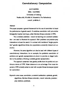
Fig. 2. Process of Coevolutionary Genetic Algorithm
3* **14 1** *
H-Individual P-Individual
schema
transcription
Superposition
3 2 1 04 02 2 312 1
H-Indiv. Superposed Individual (a) Host Dependent
3 2 1 14 02 2 112 3 Superposed H-Individual
schema
Fig. 3. Mechanism of superposition operator
Random-Sampled Individual in the schema (b) Random-Sampling
Framework We adopt Coevolutionary Genetic Algorithm to solve CSPs. As depicted in Fig.2, we have two GA populations: H-GA (Host GA) and P-GA (Parasite GA). The H-GA is a traditional GA, in other words, it searches for good solutions in the given problem. In this paper, as the traditional GA, we use SGA including roulette wheel selection with elite strategy, two point crossover and normal mutation. The P-GA searches for the good schemata in the H-GA. Each individual in P-GA consists of the alleles of H-Indiv.’s, and “∗” representing a schema in the H-GA. As depicted in the figure, two genetic operators, i.e., superposition and transcription, play the role to communicate (propagate) genetic information between the H-GA and the P-GA. These operators are described following subsections. Superposition Operator The individuals of the P-GA called P-individuals (P-indiv.’s) represent schemata in the H-GA. Namely, each P-indiv. consists of the alleles used in H-GA and “∗” (don’t care symbol), which represent a schema in the H-GA. The superposition operator copies the genetic information of a P-indiv.e xcept for “don’t care symbol” (“∗”), onto one of the individuals of H-GA called H-individuals (H-indiv.’s) in order to calculate the fitness of the P-indiv. Thus, the evolutionary process of this layered population can be regard as a coevolution of individual at different levels of abstraction (cf. Fig. 2). Fitness Evaluation of P-GA P-GA searches for useful schemata in H-GA. Here, the useful schemata in H-GA may be defined as follows: (1) undiscovered useful schemata or simply (2) useful schemata, i.e., those with high average fitness values. If we can discover schemata denoted in (1), the evolution of H-GA is promoted and guided into satisfiable solutions by suggesting the genetic information of the schemata. Also, from a point of view of constraint satisfaction, useful schemata in the sense of (2) are approximated by the evaluation of consistency between the specified gene. In this paper, we introduce three methods of the fitness evaluation for P-indivduals, called (a) HostDepended, (b) Random-Sampled, and (c) Constraint-
partial solution (schema)
Consistency check among specified variables (c) Constraint-Satisfaction
Fig. 4. Depictions of Fitness Evaluation for P-Indiv.
Satisfaction, respectively. These methods are described as follows: (a) Host-Dependent If a schema information discovered by P-GA is already discovered by H-GA, the H-GA will receive no effective information from this “discovery” by P-GA. Hence, we let P-GA to search for “undiscovered” useful schemata in HGA, and the fitness evaluation of a P-indiv. is given as follows: First, the fitness value Fj of a P-indiv., say, j is calculated in the following way where the fitness function of H-indiv. i and Pindiv. j are represented as fi and Fj , respectively. The superposing (superposition) operation of each P-indiv. onto H-indiv.’s is carried out ntry times. (i) First, ntry H-indiv.’s to be superposed by P-indiv. j are randomly selected. (ii) These selected H-indiv.’s are denoted as i1 , . . ., in , and the resultant superposed H-indiv.’s are denoted as ˜i1 , . . ., ˜in . (iii) Then, to calculate the fitness value of P-indiv. j, the effect of each of the superposition operations is evaluated as the contribution of the superposition operation to each H-indiv. defined as follows: j FHD =
ntry X
max(0, f˜ik − fik ),
(k = 1, . . . , n) .
k=1
That is, “positive contribution” of this superposition operation. If the difference is negative, then the contribution of this operation is regard to be 0. (b) Random-Sampling Generally speaking, the fitness value of a schema is calculated as the average fitness value of all individuals belonging to the schema. It is difficult, however, to calculate the fitness values of all individuals when the order of schemata is small. In this manner, the fitness
P-indiv. ordering randomly
choosing allel which is minimizing the number of constraint violations against "3" choosing allel which is minimizing the number of constraint violations against "3"&"4"
*
1
*
3
2*
*
3
*
1
2
1
2
*
4
2
1
2
*
4
1
*
3
1
*
3
*
3
*
4
re-order to original ordelring
3
tion operation is given as ( ˆk Pparasite fmaxf−f , fˆk > 0 min Ptranscription = 0 otherwise,
* 4
* 3
4
*
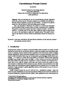
*
Fig. 5. Process of our Genetic Repair Operator for P-indiv. value is calculated as follows: (i) First, new genetic information k is generated by substituting “don’t care symbol” to alleles randomly selected. Then, the fitness value of the genetic information is calculated ntry times iteratively and the fitness value of P-Indiv. is defined as the accumulation of the fitness values, that is, j FRS =
ntry X
fk .
k=1
(c) Constraint-Satisfaction When we adopt GAs to solve CSPs, we can regard schemata as partial solutions, and can inspect the consistency of labels involved in the partial solution whether constraints are satisfied or not. In this fitness evaluation method, the satisfaction difficulty of 2compound constraint between variables i, k is defined as follows: � if constraint is violated − log T1ik fpik = 1 otherwise, log 1−T ik where, Tik denote the proportion of negative constraints. Hence, fitness of P-indiv. is given by X j fpik , FCS = i,k∈sp(j)
where, sp(j) denote the set of specified gene loci in certain P-indiv. However, it should note that every partial satisfiable solutions are not always contained in satisfiable solutions. Transcription Operator The transcription operator serves as means of transmitting the effective genetic information searched by the P-GA to the H-GA. This operator propagate genetic information in P-GA to H-Indiv. by probabilistically replacing the original H-indiv. ik with superposed H-indiv. ˜ik . The probability of applying the transcrip-
where fmax and fmin denote the maximum fitness value and the minimum fitness value in the H-GA, respectively, and hence Pparasite is set to be constant such that 0 < Pparasite < 1. Genetic Repair Operator P-GA is able to assemble good solutions from partial solutions effectively, provided that such partial solutions are consistent. Hence, we adopt Genetic Repair Operator (GRO) to keep consistency of P-individual, namely, partial solutions or schemata. As depicted in Fig. 5, the processes of this operator are carried out as follows: First, for each specified gene locus, the ordering of repair is randomly assigned, where a specified gene locus denotes a gene locus which is not assigned to ‘don’t care symbols’. The reason why the ordering is randomly assigned is to avoid converging into certain local optima. Next, according to this ordering, repair method based on consistency check is performed such that the number of constraint violations between a gene in the present order and genes in the previous order is minimized. In section 4, we will adopt two kinds of GRO as the genetic operator of the P-GA, namely, the GRO described above and GRO with mutation. The GRO with mutation adopts the ordinal mutation operator as pre processor of GRO in order to keep diverse and consistent genetic information in the P-GA population. 4. EXPERIMENTAL RESULTS In this paper, we carry out several experiments based on various general CSPs that are generated randomly for a wide variety of “density” and “tightness” of constraint conditions in the CSPs that are the basic measures of characterizing CSPs and are described in section 2. The general CSPs are randomly generated as follows: First, specify the tightness and density in the sense in section 2. Next, for all combination of two indices, decide whether unit constraint relation is set to each of the pairs of variables by taking account of the value of density. Finally, for all unit constraint relations, the number of the unit-label constraint relationships is set to be directly proportional to the tightness. In first and second experiments, general CSPs with 50 variables such that the size of domains for each of variables is set to be 10 are examined. Also, as GA parameters, following settings are used: The population size of SGA, H-GA and P-GA are set to be 200, 150 and 50, respectively. The GA parameters for the SGA and the H-GA are set to be of the same value, the probability Pc of crossover, the probability Pm of
���
��
��
��
�������
�������
�������
�������
�
�
�
�
���
���
���
���
���
���
���
���
���
���
���
���
��
��
��
��
��
��
��
��
���
���
���
��
���
��
���
�
��
���
��
�����������
������� � � � � � � � � � � � � � � �� �� �� �� �� �� �� � � � � � � � �� �� ��������� � � � � � � �� �� �� �� � � � � � � � � �� �������
���
���
��
��
���
��
�����������
�
������� � � � � � � � � � � � � � � �� �� �� �� �� �� �� � � � � � � � �� �� ��������� � � � � � � �� �� �� �� � � � � � � � � �� �������
���
��
���
�����������
�
���
�����������
�
������� � � � � � � � � � � � � � � �� �� �� �� �� �� �� � � � � � � � �� �� ��������� � � � � � � �� �� �� �� � � � � � � � � �� �������
������� � � � � � � � � � � � � � � �� �� �� �� �� �� �� � � � � � � � �� �� ��������� � � � � � � �� �� �� �� � � � � � � � � �� �������
Fig. 6. Temporal behavior of the maximum firnss in the populations: SGA (1st COLUMN), CGA with Host-Dependent (HD, 2nd COLUMN), CGA with Random-Sampling (RS, 3rd COLUMN) and CGA with Constraint-Satisfaction (CS, 4th COLUMN); the horizontal, vertical and depth axes in these graphs denote the variety of density and tightness, maximum fitness value and the number of generations
mutation and the numbers of the elitist are set to be 0.8, 0.01 and 5, respectively. Those for the P-GA are set to be Pc = 0.8 and Pm = 0.05. The elitist strategy is not used in the P-GA. Also, the number of runs for each of the tuple (tightness, density) is set to be 100. First of all, we compare SGA with each of our CGAs using different fitness evaluation for P-indiv., i.e., host-dependent (HD), random-sampling (RS) and constraint satisfaction (CS), in terms of the changes of best fitness for various values of density and tightness. In this experiments, the GRO described in previous section are not adopted. Fig. 7 shows simulation results for this experiment. The graphs in this figure denote the results for SGA, HD, RS and CS, respectively. The horizontal, vertical and depth axes of these graphs indicate the kinds of couples of density and tightness, maximum fitness value in the SGA or H-GA population for each generations, and the number of generations, respectively. As depicted in this figure, our CGA with HD outperforms the others. In tight problems, such tendencies are notable. In loose constraint problems, otherwise, the performance of them is almost similar. The reason why such phenomena are observed is regarded as follows: it is easily possible that satisfiable partial solutions are contained in satisfiable solutions in more tight problems. Moreover, it is difficult to discover such satisfiable partial solutions in more tight problems. That is, to find partial satisfiable solutions is very significant in more tight problems. Our hostdependent fitness evaluation method for the P-GA evaluates the ”contribution” of a superposition operator. Next, we apply GRO and GRO with mutation to the CGA with HD. As depicted in Fig. 7, by applying the GRO to P-GA, CSPs are solved quite effectively. The GRO can discover partial satisfiable solutions rapidly, hence the performance of the CGA is improved ex-
���������
��������� � �
�������
�������
�
�
���
���
���
���
���
���
��
��
��
��
���
��
���
���
��
���
�
��
���
��
�����������
������� � � � � � � � � � � � � � � �� �� �� �� �� �� �� � � � � � � � �� �� ��������� � � � � � � �� �� �� �� � � � � �� �� �� �������
���
�����������
�
������� � � � � � � � � � � � � � � �� �� �� �� �� �� �� � � � � � � � �� �� ��������� � � � � � � �� �� �� �� � � � � �� �� �� �������
Fig. 7. Temporal behavior of the maximum firnss in the populations: HD with repair (HD+repair, 1st COLUMN) and HD with repair + mutation (HD+repair+mut, 2nd COLUMN)
tremely. Moreover, in loose constraint problems, the GRO with mutation can solve CSPs effectively. It is terrible difficult to solve such problems because, even if we can find partial satisfiable solutions, it is rarely involved in satisfiable solutions. Namely, almost optima in such problems are not global optima, i.e., satisfiable solutions, but local optima. However, by incorporating a mutation operator into Genetic Repair Operator, the P-GA population can keep both the diversity and the consistency of genetic information. Also, we investigate the sensitivity of the parameter ntry which denotes the number of the superposition operators for a P-individual. A comparison based on the changes of maritimum fitness in H-GA population and P-GA population is shown in Fig. 8. As depicted in this figure, the parameter ntry varies from 5 to 50 for the couple (density and tightness) = (70, 70). The upper graph and lower graph in the figure denote
q
Max Fitness
1 0.8 ntry= 5 ntry=10 ntry=20 ntry=50
0.6
p q
Max Fitness
0.4 0.6
p
ntry= 5 ntry=10 ntry=20 ntry=50
0.4 0.2 0
0
50 Generations
p
100
Fig. 9. A depiction of “latent” structured CSPs
Fig. 8. Experimental results on General CSP: the average value of maximum fitness in the H-GA (UPPER) and the P-GA (LOWER)
5. CONCLUSION For various values of density and tightness, computer simulations confirmed us the effectiveness of our CGA in terms of the number of fitness evaluations and the success ratio. Especially, for tight CSPs, the repair operator worked quite effectively. In tight CSPs, it is usually very difficult to discover satisfiable schemata. Moreover, such satisfiable schemata involve useful information in searching for satisfiable solutions, provided that such schemata could have been discovered. The repair operator could discover such schemata quite well. Also, we examined “structured” CSPs involving latent “cluster” structures among the variables in the CSPs. That is, the variables in the CSPs are composed of several tightly interconnected clusters that are weak-
Max Fitness
the changes of the maximum fitness in the H-GA population and the P-GA population, respectively. The upper graph in this figure shows that the search performances against various ntry are roughly the same as each other. Because of computational effort, ntry is set to be 5. Finally, we examined “structured” CSPs involving latent “cluster” structures among the variables in the CSPs. That is, the variables in the CSPs are composed of several tightly interconnected clusters that are weakly connected with each other. As depicted in Fig. 9, cluster structured CSPs used in this paper are generated by two parameters p and q, where p denote a proposition which decides connectivity between cluster CSPs, and q denote the tightness between two variables in certain cluster CSPs. In this paper, the parameters p and q are set to 30 and 80, respectively. Our CGA can solve such structured problems very well through detecting such clusters by naturally reflecting them as P-Indiv.’s (schemata in H-GA) as depicted in Fig. 10. The GRO with mutation might serve as a mean of detector for latent schemata strucure.
0.95
0.8
0.65
SGA HD+repair w mut HD+repair HD
0.5 0
20
40 60 Generations
80
100
Fig. 10. the changes of maximum fitness in the H-GAs and SGA for structured CSPs
ly connected with each other. Our CGA could solve such structured problems very well through detecting such clusters by naturally reflecting them as P-Indiv.’s (schemata in H-GA). We also examind various methods of evaluating the fitness values of P-Indiv.’s, which elucidated the characteristics of our CGA. References [1] [2] [3] [4] [5]
[6] [7]
E. Tsang: “Foundation of Constraint Satisfaction”, Academic Press, 1993. D. E. Goldberg: “Genetic Algorithm in Search, Optimization, and Machine Learning”, Addison-Wesley, 1989. W. D. Hills: “Co-Evolving Parasites Improve Simulated Evolution as an Optimization Procedure”, Artificial Life II, pp.313-324, 1992. J. Paredis: “Co-evolutionary Constraint Satisfaction”, Proc. of PPSN III, pp.46-55, 1994. R. G. Reynolds and C. Chung: “A Self-adaptive Approach to Representation Shifts in Cultural Algorithms”, Proceedings of the 3rd International Conference of Evolutionary Computation, pp.94-99, 1996. A. N. Aizawa: “Evolving SSE: A Stochastic Schemata Exploiter”, Proceedings of the 1st International Conference of Evolutionary Computation, pp.525-529, 1994. H. Handa, N. Baba, O. Katai, T. Sawaragi and T. Horiuchi: “Genetic Algorithm involving Coevolution Mechanism to Search for Effective Genetic Information”, Proceedings of the 4th International Conference on Evolutionary Computation, pp.709-714, 1997.