Cognitive Network Interference- Modeling and ... - Semantic Scholar

This full text paper was peer reviewed at the direction of IEEE Communications Society subject matter experts for publication in the IEEE ICC 2011 proceedings

Cognitive Network Interference - Modeling and Applications Alberto Rabbachin∗ , Tony Q.S. Quek† , Hyundong Shin‡ and Moe Z. Win§ ∗ Joint

Research Centre European Commission 21027 Ispra, Italy, for Infocomm Research, A∗ STAR, 1 Fusionopolis Way, #21-01 Connexis, Singapore 138632, ‡ Department of Electronics and Radio Engineering, Kyung Hee University, 446-701 Korea, § Massachusetts Institute of Technology Cambridge, MA 02139, USA.

† Institute

Abstract—Opportunistic spectrum access creates the opening of under-utilized portions of the licensed spectrum for reuse, provided that the transmissions of secondary radios do not cause harmful interference to primary users. Therefore, it is important to characterize the effect of cognitive network interference due to such secondary spectrum reuse. In this paper, we show how a new statistical model for aggregate interference of a cognitive network, which accounts for the sensing procedure, secondary spatial reuse protocol, and environment-dependent conditions such as path loss, shadowing, and channel fading can be used to assess the aggregate interference in specific environments. Specifically, we consider scenarios like power controlled primary network, secondary network with interference avoidance mechanism, and non-circular coverage region.

I. I NTRODUCTION Opportunistic spectrum access creates the opening of underutilized portions of the licensed spectrum for reuse, provided that the transmissions of secondary radios do not cause harmful interference to primary users. To enable secondary users to accurately detect and to access the idle spectrum, cognitive radio (CR) has been proposed as the enabling technology [1]– [3]. Moreover, the CR network can implement a detect-andavoid protocol where the transmission power levels of the CR devices are based on the sensed power of the primary network signals. Spectrum sharing is however challenging due to the uncertainty associated with the aggregate interference in the network. Such uncertainty can be resulted from the unknown number of interferers and unknown locations of the interferers as well as channel fading, shadowing, and other uncertain environment-dependent conditions [4], [5]. Therefore, it is crucial to incorporate such uncertainty in the statistical interference model in order to quantify the effect of the cognitive network interference on the primary network system performance.1 A unifying framework for characterizing the network interference was proposed to investigate a variety of issues involving aggregate interference generated asynchronously in a wireless environment subject to path loss, shadowing, and multipath fading [6]. This framework has also been used 1 Throughout this paper, we refer to the aggregate interference generated by secondary users sharing the same spectrum with the primary user as cognitive network interference.

to study the coexistence issues in heterogeneous wireless networks [7]–[11]. To address the coexistence problem arose by secondary cognitive networks, it is of great importance to accurately model the aggregate interference generated by multiple active secondary users in the network [12]–[15]. In this paper, we briefly discuss our cognitive interference model proposed in [16], which accounts for sensing procedure, secondary spatial reuse protocol, and environment-dependent conditions like path loss, shadowing, and channel fading. We show how this model can be applied into different scenarios like a primary network with power control and a secondary network with interference avoidance mechanism. Moreover, our framework allows us to model the cognitive network interference generated by secondary users in a limited or finite region, taking into account the shape of the region and the position of the primary user. As an example, we show how our model can be used to analyze the aggregate interference generated by femtocell base stations. The paper is organized as follows. Section II presents the system model. Section III derives the instantaneous interference distribution. Section IV demonstrates applications of our statistical model for cognitive network interference. Section V provides numerical results to illustrate the effectiveness of our framework for characterizing the coexistence between primary and secondary networks in terms of various system parameters. Section VI gives the conclusion. II. S YSTEM M ODEL For cognitive networks, the secondary users need to sense channels before transmission in order not to cause harmful interference to a primary network. In this paper, we consider the primary network in frequency division duplex mode. Therefore, to detect the presence of active primary users, the secondary user senses the primary users’ uplink channel. Furthermore, we consider the secondary network as a simple ad-hoc network where secondary users join or exit the network, and sense or access the channel independently without coordinating with other secondary users As such, there exists the possibility that secondary users can transmit at the

978-1-61284-231-8/11/$26.00 ©2011 IEEE


same time regardless of their distances between each other.2 A. Cognitive Network Activity Model The activity of each secondary user depends on the strength of the received uplink signal transmitted by the primary user. In the following, we consider a single-threshold protocol. In this case, the ith secondary user is active if KPp Yi ≤ β, Ri2b

(1)

or equivalently, Ri−2b Yi ≤ ζ,

(2)

is the normalized where β is the activating threshold; ζ threshold; Pp is the transmitted power of the primary user; Yi is the squared fading path gain of the channel from the primary user to the ith secondary user; K is the gain accounting for the loss in the near-field; Ri is the distance between the primary and the ith secondary user; and b is the amplitude pass-loss exponent.3 We assume that Yi ’s are independent and identically distributed (IID) with the common cumulative distribution function (CDF) FY (·). Therefore, the activity of the secondary network users can be represented by the Bernoulli random variable: (3) 1[0,ζ] Ri−2b Yi ∼ Bern FYi Ri2b ζ , β KPp

with the indicator function defined as 1, if p ≤ x ≤ q 1[p,q] (x) = 0, otherwise,

P {|S| = k} =

(λAR )k −λAR e , k!

B. Interference Model The interference signal at the primary receiver generated by the ith cognitive interferer can be written as (5) Ii = PI Ri−b Xi , where PI is the interference signal power at the limit of the near-far region;4 Ri is the distance between the ith cognitive interferer and the primary receiver; and Xi is the perdimension fading channel path gain of the channel from the ith cognitive interferer to the primary receiver.5 In the following, we assume that Xi ’s are IID with common probability density function (PDF) fX (·), which are mutually independent of Yi ’s. We consider that the secondary users are spatially scattered according to an homogeneous Poisson point process in a two-dimensional plane R2 , where the victim primary user is assumed to be located at the center of the region. Let S ⊂ Z+ a more intelligent medium access control protocol that involves a form of coordination or local information exchange is feasible for the secondary network, our results can still serve as a worst-case scenario analysis. 3 For brevity, we assume that the noise effect is negligible on the primary detection procedure as in [14]. 4 We consider the near-far region limit at 1 meter. 5 Note that X = {H }, where H is the complex path gain of the channel i i i from the ith cognitive interferer to the primary receiver.

k = 0, 1, 2, . . .

(6)

where λ is the spatial density (in nodes per unit area). Furthermore, we assume that the region R is constrained in the annulus prescribed by two radius dmin and dmax , which are minimum and maximum distances from the primary receiver, respectively.6 This allows us to consider a scenario where the secondary users are located within a limited region. III. I NSTANTANEOUS I NTERFERENCE D ISTRIBUTION To characterize the cognitive network interference, we derive the cumulants for the cases of full network activity (all secondary users are active) and regulated activity (each secondary user is regulated by a spatial reuse protocol) in Section III-A and III-B, respectively. A. Full Activity In this case, the cognitive network interference is generated by all the secondary users present in the region R and can be written as −b PI Ri Xi . (7) Ifa = i∈S

(4)

where the value one of the Bernoulli variable denotes that the secondary user is active.

2 When

be the index set of secondary users in a region R ⊂ R2 . Then the probability that k secondary users lie inside R depends only on the total area AR of the region, and is given by [17]

Zfa

By using [6, Theorem 3.1], the CF of Zfa can be expressed as dmax

1 − exp jωxr−b ψZfa (jω) = exp −2πλ X

dmin

×fX (x) rdrdx) ,

(8)

√ where j = −1. Using (8), we can then calculate the nth cumulant of the interference Zfa as follows: 1 dn ln ψZfa (jω) κZfa (R) (n) = jn dω n ω=0 dmax = 2πλ xn r1−nb fX (x) drdx X

=

dmin

2πλ 2−nb d μX (n) . − d2−nb max nb − 2 min

(9)

Using the cumulant of Zfa (R), we can obtain the nth cumulant of the cognitive network interference Ifa for the full activity case as follows: n/2

κIfa (n) = PI

κZfa (R) (n) .

(10)

6 Note that R in (5) can be smaller than 1. Therefore, the received i interference power can be larger than PI but it is finite since dmin > 0.


B. Regulated Activity - Single-Threshold Protocol In this spatial reuse protocol, the activity of the secondary users in the region R is regulated by the single normalized threshold ζ according to (3). Therefore, the cognitive network interference for the single-threshold protocol can be written as −b PI Ri Xi , (11) Ist = i∈Ast

Zst (ζ;R)

where Ast defines the index set of active secondary users in the region R: (12) Ast = i ∈ S : 1[0,ζ] Ri−2b Yi = 1 .

perfect power control, Pp is set such that Pp |Hp |2 /(Rp2b ) ≥ P , where P is the minimum required power level. For discrete power control, the set of possible power levels are finite. Assuming that there are L possible transmit power levels P1 , P2 , . . . , PL , we have the following probability mass function (PMF) for Pp at these power levels: P {Pp = P } = ⎧ 2b P Rp ⎪ ⎪ for = 1, ⎪ ⎪P |Hp |2 ≤ P1 , ⎪ ⎪ ⎨ P R2b P P−1 < |Hp |p2 ≤ P , for = 2, 3, . . . , L − 1, ⎪ ⎪ ⎪ 2b ⎪ P Rp ⎪ ⎪ for = L, ⎩P |Hp |2 > PL ,

Similar to (8), the CF of Zst (ζ; R) can be expressed as ψZst (ζ;R) (jω) =

exp −2πλ

X

Y

dmax

(17)

1 − exp jωxr−b

dmin

× 1[0,ζ] r−2b y fX (x) fY (y) rdrdydx , (13) from which the cumulant κZst (ζ;R) (n) can be derived and expressed as follow: κZst (ζ;R) (n) =

2πλ μX (n) 2−nb dmin − d2−nb FY d2b max min ζ nb − 2 nb−2 2 − nb 2b (pt) 2b 2b , dmin ζ, dmax ζ +ζ μY 2b 2b 2−nb (pt) 2b 0, dmin ζ, dmax ζ . − dmax μY (14) Using the cumulant of Zst (ζ; R), we can obtain the nth cumulant of the cognitive network interference Ist for the single-threshold protocol as follows: n/2

st

n/2

= PI

L

KPp

P {Pp = P } κZ

=1

st

β KP

;R

(n) .

(18)

B. Effect of Secondary Interference Avoidance

κIst (n) = PI

which can be determined empirically. In this case, the nth cumulant of the cognitive network interference for the singleβ . threshold protocol can be written as where ζ = KP n/2 κIst (n) = E PI κZ (n) β ;R

κZst (ζ;R) (n) .

(15)

Remark 1: As ζ → ∞, the second and third terms in (14) vanish and hence, lim κIst (n) = κIfa (n) ,

ζ→∞

(16)

as expected. Therefore, the full activity can be viewed as an extreme case of the single-threshold spatial reuse such that ζ → ∞. IV. A PPLICATIONS A. Effect of the Primary Network Power Control Power control is often used in cellular systems to overcome the near-far problem. If the primary network uses power control, the transmitting power of the primary user varies depending on the distance Rp and channel gain Hp between the base station and primary receiver. Therefore, the transmit power Pp is random and it is important to understand the effect of power control on the cognitive network interference. Under

Instead of allowing all the active secondary users in the same class to transmit at the same power, we can also employ secondary power control, which will be effective in reducing interference and improving power efficiency [18], [19]. In addition, we can effectively design a more power-efficient secondary network if the knowledge of the secondary users’ positions is available. For example, each secondary user avoids transmitting using on-off power control if the average received signal-to-noise-ratio at its desired receiver is very low. Hence, with the location-awareness, we can regulate each secondary user to transmit only if its desired secondary receiver is within a certain maximum transmission range R , which corresponds to the maximum distance beyond which reliable transmission is not possible. Let Ps and Rs be the random variables that represent the secondary transmit power and the distance from the intended receiver, respectively. Then, for the singlethreshold spatial reuse protocol with power control, the nth cumulant of the cognitive network interference becomes:7 κIst (n) = μ√Ps (n) κZst (ζ;R) (n) .

(19)

If the intended receiver is the nearest neighbor, then Rs ∼ Rayleigh (1/ (2πλr )) follows from the properties of Poisson point processes, where λr is the density of secondary receivers. 7 The nth moment μ√ (n) depends on the power control and intended Ps receiver selection strategies of the secondary network. For example, we have Ps ∼ PI Bern (FRs (R )) for the on-off secondary power control with the maximum transmission range R . Hence, n/2

μ√Ps (n) = PI n/2

and μ√Ps (n) → PI

FRs (R ) ,

as R → ∞ (no power control).


Aggregate interference power [dBm] 30 −20 meters

25 −40

20

−60

15 10 10

20

30

40

50

60

−80

meters

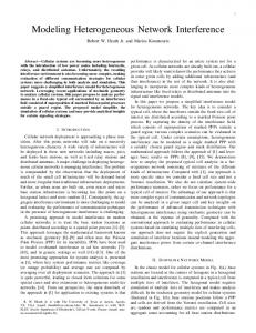
Fig. 1. Circular-section approximation of the non-circular region. The green square represents the primary user. Different colored sections correspond to different secondary user densities.

Fig. 2. Aggregate interference power generated by femtocell base stations placed with density λ = 0.01 users/m2 in the first and third apartment of the row above and in the third and fifth apartment of the row below for PI = 0 dBm, walls absorbing 20 dB of the radio signal, and |Hi | ∼ Nakagami (2, 1).

expressed as C. Non-circular Regions When the primary and secondary users are confined in a limited or finite region, the position of the primary user and the shape of the region affect the distribution of the distance between the primary and secondary users and, therefore, also that of the aggregate interference. In the framework developed in Sections II and III, we implicitly consider the polar coordinate system and place the primary user at the center of the region. This coordinate system is natural for analyzing the interferers scattered in a circular section. To extend this framework to a non-circular region, we can first divide the area of interest into infinitesimal circular sections (see for example, Fig. 1) and use (23) to approximate the nth cumulant of the cognitive network interference. Using this approach, we can also consider any position of the primary user, shadowing with multiple obstacles, and areas with different densities within the region of interest. For example, consider the single-threshold protocol in an non-circular environment with obstacles and regions with different densities such that the whole region R can be divided into different subregions R0 , and R1 , R2 , . . . , RL . Due to presence of the obstacles, some of these L subregions experience additional attenuation behind those obstacles. Then, the cognitive network interference can be written as

Ist

=

L =0

PI,

Ri−b Xi ,

i∈Ast,

Zst (ζ β˘ ;R )

(20)

where Ast, = i ∈ S ∩ R : 1[0,ζ β˘ ] Ri−2b Yi = 1 .

(21)

For = 1, 2, . . . , L, PI, and β˘ account for an additional attenuation if the subregion R is behind the obstacle, and PI,0 = PI and β˘0 = 1. The CF of Zst ζ β˘ ; R ) can be

ψZst (ζ β˘ ;R ) (jω) = exp −θ λ

1[0,ζ β˘ ] r

X

−2b

Y

b

1 − exp jωxr−b

a

y fX (x) fY (y) rdrdydx .

(22)

where a and b are the limits of the subregion R ; λ is the node density in the subregion and θ is the angle covered by R . If the obstacle is present, the angle θ corresponds to the angle covered by the obstacle. For a single obstacle placed at distance d from the origin, we have two subregions in front and behind the obstacle: (a1 , b1 ) = (dmin , d) and (a2 , b2 ) = (d, dmax ), respectively. The nth cumulant of the cognitive network interference for the single-threshold protocol in the presence of shadowing can be written as κIst (n) =

L =0

n/2

PI, κZst (ζ β˘ ;R ) (n)

(23)

where the cumulant κZst (ζ β˘ ;R ) (n) is obtained from κZst (ζ;R) (n) in (14) by replacing ζ, 2π, dmin , and dmax with ζ β˘ , θ , a , and b , respectively. 1) Femtocells: With the approach proposed for non-circular regions, the aggregate interference model can be used to measure the aggregate interference generated by femtocells. Femtocells form underlay networks that are used to extend the range and to enhance the network capacity of macrocell cellular networks. Femtocell base stations are deployed in an uncoordinated manner to increase the coverage and network capacity of the macrocell network [20]. Since femtocell base stations are randomly placed and are not coordinated among them with the macrocell network, they can become a potential cause of harmful interference to the macrocell users. It is then of great importance to assess the interference generated by femtocell base stations taking into account the environment where the base stations are deployed. The state-of-the-art technology do not consider cognitive femtocell base stations, therefore by using the tool defined in (23) with the cumulants expressed for the full network activity by (9) instead of κZst (ζ β˘ ;R ) (n) allows to characterize the statistics of the


0

0.3

10

PU at the center of the square PU at the center of the low density region PU at the up-right corner of the square

power control on power control off

0.25 10

0.07

0.2

0.06 fIfa (x)

Cognitive network interference

−1

−2

10

0.15 0.05 0.1

0.04

−3

10

−0.1−0.05 0 0.05 0.1 0.05

−4

10

−6

−5

10

−4

10

−3

10

−2

10

10

Activating threshold β Fig. 3. Variance of the cognitive network interference Ist for the singlethreshold protocol in the presence of primary power control as a function of the activating threshold β. λ = 0.1 users/m2 , K = 0 dBm, PI = 0 dBm, |Hp | ∼ Rayleigh (1/2), dminp = 1 meter, and dmaxp = 1000 meters. The power levels of the primary user are −5, −15, −25, and −35 dBm with the minimum required power level P = −95 dBm.

−2

Cognitive network interference

10

−4

10

−6

10

−8

10

λ = 0.01 λ = 0.001 λ = 0.0001 λ = 0.00001

−10

10

10

20

30

40

50

60

70

80

Maximum transmission range R (meters)

90

100

Fig. 4. Variance of the cognitive network interference Ifa for full activity (ζ → ∞) in the presence of the on-off secondary power control as a function of the maximum transmission range R of the secondary users when λ = 0.01, 0.001, 0.0001, and 0.00001 users/m2 . PI = 0 dBm, Ps ∼ Bern (FRs (R )), Rs ∼ Rayleigh (1/ (2πλ√ r )), λr = λ, and Nakagamim fading for primary and secondary links Yi ∼ Nakagami (2, 1) and |Hi | ∼ Nakagami (2, 1).

aggregate interference generated by femtocell base stations in any environment. In Fig. 2, the aggregate interference is calculated in one of the reference environment chosen in the femtocells standardization process. V. N UMERICAL RESULTS In this section, we illustrate the use of cognitive network interference model to provide insight into the coexistence

0 −1.5

−1

−0.5

0

0.5

1

1.5

x Fig. 5. PDF of the cognitive network interference Ifa at the primary user (PU) in a (200 × 200)-meter square (see Fig. 1) for full activity (ζ → √ ∞). PI = 0 dBm and Nakagami-m fading for primary and secondary links Yi ∼ Nakagami (2, 1) and |Hi | ∼ Nakagami (2, 1). The secondary spatial density is equal to λ = 0.01 users/m2 in the red sections, whereas λ = 0 users/m2 (i.e., no secondary users) in the yellow sections.

between primary and secondary networks. In numerical examples, we consider dmin = 1 meter, dmax = 60 meters, b = 1.5, and Rayleigh fading for both primary and secondary signals unless differently specified. The effect of power control on the cognitive network interference is illustrated in Fig. 3, where the variance of the cognitive network interference Ist for the single-threshold protocol as a function of the activating threshold β is depicted in the presence of primary power control. In this example, K = 0 dBm and the density and transmit power of the secondary users are λ = 0.1 users/m2 and PI = 0 dBm, respectively. The primary user is distributed in a circular area defined by minimum and maximum distances dminp = 1 meter and dmaxp = 1000 meters from the base station, respectively, and its communication link experiences Rayleigh fading, i.e., |Hp | ∼ Rayleigh (1/2). For the primary power control policy, we set four power levels −5, −15, −25, −35 in dBm and the minimum required power level to P = −95 dBm. We can see from the figure that if the primary network uses power control, the variance of the cognitive network interference increases for all the values of β. This is due to the fact that when the primary user is close to the base station, its transmission power decreases. As a consequence, the secondary users will increase their activity, leading to a larger number of active secondary users. In Fig. 4, the variance of the cognitive network interference Ifa as a function of the maximum transmission range R of the secondary users for the case of full activity (i.e., ζ → ∞) is depicted in the presence of the on-off secondary power control for various values of λ. In this example, √ Yi ∼ Nakagami (2, 1) and |Hi | ∼ Nakagami (2, 1). For the secondary power control policy, we set PI = 0 dBm,


Ps ∼ Bern (FRs (R )), Rs ∼ Rayleigh (1/ (2πλr )), and 2 λr = λ. Hence, μ√Ps (n) in (19) becomes 1−e−πλr R , which reveals that the interference power increases and approaches exponentially to one (i.e., PI = 0 dBm without power control) as the transmission range R increases. We can see from Fig. 4 that the cognitive interference power reduces, especially at low values of λ, as the range R decreases. Fig. 5 shows the PDFs of the cognitive network interference Ifa at the primary user in a (200 × 200)-meter square (see Fig. 1) for the case of full activity (ζ → ∞) and PI = 0 dBm. The √ primary and secondary links have Nakagami-m fading, i.e., Y ∼ Nakagami (2, 1) and |Hi | ∼ Nakagami (2, 1); and the square region has two different secondary spatial densities: λ = 0.01 in the red sections and λ = 0 (i.e., no secondary users) in the yellow sections. The PDFs fIfa (x) are plotted for three cases of the primary user location: i) at the center of the large square, ii) at the center of the low (zero) density region, and iii) at the up-right corner of the large square. We can observe from Fig. 5 that the the cognitive network interference becomes less severe as the primary user moves to the corner. This is due to the fact that the distance between the primary and secondary users increases when the primary user is located at the corner. Moreover, using this framework, we can also consider a nonuniform spatial distribution of the secondary users in the region of interest. Therefore, our statistical interference model enables us to characterize the position where the primary user is less vulnerable to the effect of cognitive network interference. VI. C ONCLUSIONS In this paper, we showed how our statistical model for aggregate interference of cognitive networks, which accounts for the sensing procedure, the spatial distribution of nodes, secondary spatial reuse protocol, and environment-dependent conditions can be applied in different scenarios. In particular, we considered scenarios like a primary network with power control, a secondary network with interference avoidance mechanism, and network with non-circular coverage regions. The framework developed here enables us to characterize cognitive network interference for successful deployment of future cognitive networks. Lastly, we showed how our proposed model can also be used to analyze the effect of inter-tier interference in femtocell networks. R EFERENCES [1] FCC, “Notice of proposed rule making, in the matter of facilitating opportunities for flexible, efficient and reliable spectrum use employing cognitive radio technologies (et docket no. 03-108) and authorization and use of software defined radios (et docket no. 00-47), FCC 03-322,” FCC, Tech. Rep., 2003. [2] S. Haykin, “Cognitive radio: brain-empowered wireless communications,” IEEE J. Select. Areas Commun., vol. 23, no. 2, pp. 201–220, Feb. 2005. [3] A. Goldsmith, S. A. Jafar, I. Maric, and S. Srinivasa, “Breaking spectrum gridlock with cognitive radios: An information theoretic perspective,” Proc. IEEE, vol. 97, no. 5, pp. 894–914, May 2009. [4] R. Tandra and A. Sahai, “SNR walls for signal detection,” IEEE Trans. Sel. Topics Signal Processing, vol. 2, no. 1, pp. 4–17, Feb. 2008.

[5] R. Tandra, S. M. Mishra, and A. Sahai, “What is a spectrum hole and what does it take to recognize one: extended version,” Proc. IEEE, vol. 97, no. 5, pp. 824–848, May 2009. [6] M. Z. Win, P. C. Pinto, and L. A. Shepp, “A mathematical theory of network interference and its applications,” Proc. IEEE, vol. 97, no. 2, pp. 205–230, Feb. 2009. [7] P. C. Pinto and M. Z. Win, “Communication in a Poisson field of interferers – Part I: Interference distribution and error probability,” IEEE Trans. Wireless Commun., vol. 9, no. 7, pp. 2176–2186, Jul. 2010. [8] ——, “Communication in a Poisson field of interferers – Part II: Channel capacity and interference spectrum,” IEEE Trans. Wireless Commun., vol. 9, no. 7, pp. 2187–2195, Jul. 2010. [9] A. Rabbachin, T. Q. S Quek, P. C. Pinto, I. Oppermann, and M. Z. Win, “Non-coherent UWB communication in the presence of multiple narrowband interferers,” IEEE Trans. Wireless Commun., vol. 9, no. 11, pp. 3365–3379, Nov. 2010 [10] P. C. Pinto, A. Giorgetti, M. Z. Win, and M. Chiani, “A stochastic geometry approach to coexistence in heterogeneous wireless networks,” IEEE J. Sel. Areas Commun., vol. 27, no. 7, pp. 1268–1282, Sep. 2009. [11] P. C. Pinto and M. Z. Win, “Spectral characterization of wireless networks,” IEEE Wireless Commun. Mag., vol. 14, no. 6, pp. 27–31, Dec. 2007. [12] E. Salbaroli and A. Zanella, “Interference analysis in a Poisson field of nodes of finite area,” IEEE Trans. Veh. Technol., vol. 58, no. 4, pp. 1776–1783, Apr. 2009. [13] H. Inaltekin, M. Chiang, H. V. Poor, and S. B. Wicker, “On unbounded path-loss models: effect of singularity on wireless network performance,” IEEE J. Select. Areas Commun., vol. 27, no. 7, pp. 1078–1092, Jul. 2009. [14] A. Ghasemi and E. S. Sousa, “Interference aggregation in spectrumsensing cognitive wireless networks,” IEEE Trans. Sel. Topics Signal Processing, vol. 2, no. 1, pp. 41–56, Feb. 2008. [15] R. Menon, R. M. Buehrer, and J. H. Reed, “On the impact of dynamic spectrum sharing techniques on legacy radio systems,” IEEE Trans. Wireless Commun., vol. 7, no. 11, pp. 4198–4207, Nov. 2008. [16] A. Rabbachin, T. Q. S. Quek, H. Shin, and M. Z. Win, “Cognitive network interference,” IEEE J. Select. Areas Commun., vol. 29, no. 2, pp. 480–493, Feb. 2011. [17] J. Kingman, Poisson Processes, 1st ed. Oxford University Press, 1993. [18] N. Bambos and S. Kandukuri, “Power controlled multiple access (pcma) schemes for next-generation wireless packet networks,” IEEE Trans. Commun., vol. 9, no. 3, pp. 58–64, Sep. 2002. [19] G. J. Foschini and Z. Miljanic, “A simple distributed autonomous power control algorithm and its convergence,” IEEE Trans. Veh. Technol., vol. 42, no. 4, pp. 641–646, Nov. 1993. [20] V. Chandrasekhar, J. G. Andrews, and A. Gatherer, “Femtocell networks: A survey,” IEEE Commun. Mag., vol. 46, no. 9, pp. 59–67, Sep. 2008.