Signal Processing and Communications Department. DOCTORAL ... interference
management in cognitive radio networks in which certain interaction is allowed ...
DOCTORAL DISSERTATION · 2011
INTERFERENCE AND NETWORK MANAGEMENT IN COGNITIVE COMMUNICATION SYSTEMS
Gonzalo Vázquez Vilar
University of Vigo Signal Processing and Communications Department
DOCTORAL DISSERTATION EUROPEAN MENTION INTERFERENCE AND NETWORK MANAGEMENT IN COGNITIVE COMMUNICATION SYSTEMS Author: Gonzalo V´azquez Vilar Directed by: Roberto L´opez Valcarce Carlos Mosquera Nartallo
2011
DOCTORAL DISSERTATION EUROPEAN MENTION INTERFERENCE AND NETWORK MANAGEMENT IN COGNITIVE COMMUNICATION SYSTEMS Gonzalo V´azquez Vilar Directed by: Roberto L´opez Valcarce Carlos Mosquera Nartallo
EXAMINATION COMMITTEE
President:
Fernando P´erez Gonz´alez
Board members:
Wilfried Gappmair Santiago Zazo Bello Ashish Pandharipande
Board secretary:
Josep Sala Alvarez
Thesis defense:
Vigo, June 29, 2011
This edition:
July 5, 2011
The wireless channel is a complicated animal. A. Paulraj
Research is to see what everybody else has seen, and to think what nobody else has thought. A. Szent-Gy¨orgyi
Acknowledgements First of all, I want to thank my advisors Roberto and Carlos for their guidance and encouragement in the development and preparation of this dissertation. Without them this thesis would not exist. I would also like to acknowledge all the people I met during these last two years and who participated at any point in the work of this thesis. Specially, I would like to thank Nuria Gonz´ alez Prelcic, Josep Sala, Sudharman K. Jayaweera, David Ram´ırez, and Ashish Pandharipande, as well as the members from the groups of SPCOM (Technical Univ. of Catalonia UPC) and GTAS (University of Cantabria). Additionally I want to acknowledge all the people that, through my blog Spectral Holes, helped me to understand several issues behind Cognitive Radio. I learned from all of them. Other people who have also contributed to this thesis, but in a different way, are my lab colleagues, Marcos, Norberto, Enrique, Marta, Eli and Debora. I want to thank all of them for doing my stay pleasant and enjoyable. Also my friends Yoli, Borja, Paco and Edu, who shared my lunch-time relax during this period of my life. And last but not least, I want to acknowledge the support of my family. I thank my parents, Gonzalo and Lidia, my sister, Marta, and my girlfriend Alba for their (not small) patience and (huge) love.
Abstract The key idea behind Cognitive Radio (CR) is to allow opportunistic access to temporally and/or geographically unused licensed bands, avoiding conflicts with the rightful license owners in those bands. To achieve this, novel interference management algorithms are required to limit the interference seen by the primary (licensed) users. A key aspect of any interference management scheme is spectrum monitoring, that allows to detect and track primary users. This PhD. Thesis contributes to the field of CR in two different ways. First, we address the problem of primary user monitoring using novel detection schemes which exploit multiple antennas, wideband processing, and the available a priori knowledge about primary transmissions. Then, we propose a general framework for interference management in cognitive radio networks in which certain interaction is allowed between primary and secondary systems. Specifically, the detection problems investigated in this thesis include multiantenna detection exploiting a priori spectral information when the noise statistics are assumed known. In this setting we will also derive novel diversity order analysis of the proposed detectors. The case of multiantenna detection under unknown noise statistics is covered under different hypotheses, including both the detection of primary signals with spatial rank larger than one and detection in presence of spatially unstructured noise. Additionally we study the problem of multichannel monitoring. In this context, wideband acquisition can be performed using traditional analog to digital converters or the recently proposed analog to information converters. When the channelization of the primary network is assumed known, we show that guard bands and weak channels can be used to improve detection performance, both when the detection is performed from a set of samples at Nyquist rate, or from a set of compressed measurements. Finally, we propose a general framework for interference management in cogni-
vi
tive radio networks in which the primary network is allowed to dynamically adjust the tolerable interference margin to be met by the secondary system. In particular, we propose a game theoretical formulation which allows us to study the performance gain which can be expected from this limited interaction between primary and secondary systems. Moreover, we show that certain architectures fulfilling these requirements are implementable in practice and present good performance in both static and dynamic environments.
Publications The following is a list of journal and conference publications that have been produced as a result of the work on this thesis.
Journal publications 1. Josep Sala, Gonzalo Vazquez-Vilar, and Roberto L´opez-Valcarce. Multiantenna detection in unknown spatially correlated noise in cognitive radio networks. Signal Processing, IEEE Transactions on, 2011. In review. 2. Gonzalo Vazquez-Vilar, Roberto L´opez-Valcarce, and Josep Sala. Multiantenna detection of multicarrier primary signals exploiting spectral a priori information. Wireless Communications, IEEE Transactions on, 2011. In review. 3. Gonzalo Vazquez-Vilar and Roberto L´opez-Valcarce. Wideband spectrum sensing exploiting guard bands and weak channels. Signal Processing, IEEE Transactions on, 2011. Accepted for publication. 4. David Ram´ırez, Gonzalo Vazquez-Vilar, Roberto L´opez-Valcarce, Javier V´ıa, and Ignacio Santamar´ıa. Detection of rank-P signals in cognitive radio networks with uncalibrated multiple antennas. Signal Processing, IEEE Transactions on, 2011. In press. 5. Gonzalo Vazquez-Vilar, Carlos Mosquera, and Sudharman K. Jayaweera. Primary user enters the game: Performance of dynamic spectrum leasing in cognitive radio networks. Wireless Communications, IEEE Transactions on, 9(12):3625–3629, December 2010.
vii
viii
6. Sudharman K. Jayaweera, Gonzalo Vazquez-Vilar, and Carlos Mosquera. Dynamic Spectrum Leasing (DSL): A new paradigm for spectrum sharing in cognitive radio networks. Vehicular Technology, IEEE Transactions on, 59(5):2328–2339, June 2010.
Conference publications 1. Gonzalo Vazquez-Vilar, Roberto L´opez-Valcarce, and Ashish Pandharipande. Detection diversity of multiantenna spectrum sensors. In 2011 IEEE International Conference on Acoustics, Speech and Signal Processing (ICASSP 2011), Prague, Czech Republic, May 2011. 2. David Ram´ırez, Gonzalo Vazquez-Vilar, Roberto L´opez-Valcarce, Javier V´ıa, and Ignacio Santamar´ıa. Multiantenna detection under noise uncertainty and primary user’s spatial structure. In 2011 IEEE International Conference on Acoustics, Speech and Signal Processing (ICASSP 2011), Prague, Czech Republic, May 2011. 3. Roberto L´ opez-Valcarce, Gonzalo Vazquez-Vilar, and Josep Sala. Multiantenna spectrum sensing for cognitive radio: overcoming noise uncertainty. In The 2nd International Workshop on Cognitive Information Processing (CIP 2010), Elba Island (Tuscany), Italy, June 2010. 4. Georges El-Howayek, Sudharman K. Jayaweera, Kamrul Hakim, Gonzalo Vazquez-Vilar, and Carlos Mosquera. Dynamic spectrum leasing (DSL) in dynamic channels. In ICC’10 Workshop on Cognitive Radio Interfaces and Signal Processing (ICC’10 Workshop CRISP), Cape Town, South Africa, May 2010. 5. Gonzalo Vazquez-Vilar, Roberto L´opez-Valcarce, Carlos Mosquera, and Nuria Gonz´ alez-Prelcic. Wideband spectral estimation from compressed measurements exploiting spectral a priori information in cognitive radio systems. In 2010 IEEE International Conference on Acoustics, Speech and Signal Processing (ICASSP 2010), Dallas, U.S.A., March 2010. ´ 6. Roberto L´ opez-Valcarce, Gonzalo Vazquez-Vilar, and Marcos Alvarez D´ıaz. Multiantenna detection of multicarrier primary signals exploiting spectral a
ix
priori information. In 4th International Conference on Cognitive Radio Oriented Wireless Networks and Communications (Crowncom 2009), Hannover, Germany, June 2009. 7. Roberto L´ opez-Valcarce and Gonzalo Vazquez-Vilar. Wideband spectrum sensing in cognitive radio: Joint estimation of noise variance and multiple signal levels. In 2009 IEEE International Workshop on Signal Processing Advances for Wireless Communications (Spawc 2009), Perugia, Italy, June 2009.
Contents 1 Introduction
1
1.1
Cognitive Radio: Motivation . . . . . . . . . . . . . . . . . . . . . .
1
1.2
Previous work . . . . . . . . . . . . . . . . . . . . . . . . . . . . . . .
2
1.2.1
Spectrum Monitoring . . . . . . . . . . . . . . . . . . . . . .
3
1.2.2
Interference Management . . . . . . . . . . . . . . . . . . . .
7
Contributions . . . . . . . . . . . . . . . . . . . . . . . . . . . . . . .
7
1.3.1
Multiantenna and multichannel detection of primary users . .
8
1.3.2
DSL: an Interference Management Scheme . . . . . . . . . . .
10
1.4
Structure of the thesis . . . . . . . . . . . . . . . . . . . . . . . . . .
11
1.5
Notation . . . . . . . . . . . . . . . . . . . . . . . . . . . . . . . . . .
11
1.3
2 Calibrated Multiantenna Detection
13
2.1
Introduction . . . . . . . . . . . . . . . . . . . . . . . . . . . . . . . .
14
2.2
System model . . . . . . . . . . . . . . . . . . . . . . . . . . . . . . .
14
2.3
Problem formulation . . . . . . . . . . . . . . . . . . . . . . . . . . .
17
2.3.1
Neyman-Pearson detector . . . . . . . . . . . . . . . . . . . .
17
2.3.2
Detection with multiple antennas . . . . . . . . . . . . . . . .
19
2.3.3
Generalized energy detector . . . . . . . . . . . . . . . . . . .
20
Parameter estimation and detection . . . . . . . . . . . . . . . . . .
21
2.4.1
21
2.4
Selection Combining detector . . . . . . . . . . . . . . . . . .
xi
xii
CONTENTS
2.4.2
Equal Gain Combining detector . . . . . . . . . . . . . . . . .
22
2.4.3
Maximal Ratio Combining detector . . . . . . . . . . . . . . .
24
Detection diversity in fading environments . . . . . . . . . . . . . . .
25
2.5.1
High SNR diversity order analysis . . . . . . . . . . . . . . .
26
2.5.2
Daher-Adve diversity order analysis . . . . . . . . . . . . . .
28
2.6
Numerical results and discussion . . . . . . . . . . . . . . . . . . . .
32
2.7
Conclusions . . . . . . . . . . . . . . . . . . . . . . . . . . . . . . . .
40
2.A Statistical analysis for large data records . . . . . . . . . . . . . . . .
42
2.A.1 Generalized Energy Detector . . . . . . . . . . . . . . . . . .
42
2.A.2 Selection Combining Detector . . . . . . . . . . . . . . . . . .
43
2.A.3 Equal Gain Combining detector . . . . . . . . . . . . . . . . .
44
2.A.4 Maximal Ratio Combining detector . . . . . . . . . . . . . . .
47
2.B Asymptotic analysis of gL (x) . . . . . . . . . . . . . . . . . . . . . .
48
2.5
3 Multiantenna Detection under Unknown Noise Statistics
51
3.1
Introduction . . . . . . . . . . . . . . . . . . . . . . . . . . . . . . . .
52
3.2
Problem formulation . . . . . . . . . . . . . . . . . . . . . . . . . . .
53
3.2.1
System model . . . . . . . . . . . . . . . . . . . . . . . . . . .
53
3.2.2
Hypothesis testing problem . . . . . . . . . . . . . . . . . . .
55
Detection of rank-P signals in spatially uncorrelated noise . . . . . .
56
3.3.1
Spatially uncorrelated iid noise process . . . . . . . . . . . . .
56
3.3.2
Spatially uncorrelated non-iid noise process . . . . . . . . . .
58
3.3.3
Numerical results and discussion . . . . . . . . . . . . . . . .
63
Detection of rank-1 signals in spatially correlated noise . . . . . . . .
67
3.4.1
Genie-aided detectors . . . . . . . . . . . . . . . . . . . . . .
68
3.4.2
GLRT detector . . . . . . . . . . . . . . . . . . . . . . . . . .
70
3.4.3
Asymptotic performance analysis . . . . . . . . . . . . . . . .
81
3.4.4
Numerical results and discussion . . . . . . . . . . . . . . . .
85
3.3
3.4
CONTENTS
xiii
3.5
Conclusions . . . . . . . . . . . . . . . . . . . . . . . . . . . . . . . .
88
3.A Proof of Lemma 3.2 . . . . . . . . . . . . . . . . . . . . . . . . . . .
91
T −1 . . . . . . . . . . . 3.B Detailed computation of (ILK + (hΣ hH Σ ) ⊗ C)
92
3.C Proof of Lemma 3.7 . . . . . . . . . . . . . . . . . . . . . . . . . . .
92
3.D Proof of Lemma 3.8 . . . . . . . . . . . . . . . . . . . . . . . . . . .
93
3.E Proof of Theorem 3.2 . . . . . . . . . . . . . . . . . . . . . . . . . . .
94
4 Wideband Spectrum Sensing
99
4.1
Introduction . . . . . . . . . . . . . . . . . . . . . . . . . . . . . . . . 100
4.2
Problem formulation . . . . . . . . . . . . . . . . . . . . . . . . . . . 101
4.3
4.4
4.5
4.2.1
Wideband acquisition . . . . . . . . . . . . . . . . . . . . . . 101
4.2.2
Signal model . . . . . . . . . . . . . . . . . . . . . . . . . . . 102
4.2.3
Hypothesis testing problem . . . . . . . . . . . . . . . . . . . 103
Wideband spectrum sensing at Nyquist rate . . . . . . . . . . . . . . 104 4.3.1
GLRT detection . . . . . . . . . . . . . . . . . . . . . . . . . 104
4.3.2
Orthogonal frequency-flat signals in white noise . . . . . . . . 108
4.3.3
Statistical analysis . . . . . . . . . . . . . . . . . . . . . . . . 114
4.3.4
Numerical results and discussion . . . . . . . . . . . . . . . . 116
Compressed spectrum sensing . . . . . . . . . . . . . . . . . . . . . . 121 4.4.1
Estimation from compressed measurements . . . . . . . . . . 121
4.4.2
Quasi-GLRT detection . . . . . . . . . . . . . . . . . . . . . . 127
4.4.3
Numerical results and discussion . . . . . . . . . . . . . . . . 128
Conclusions . . . . . . . . . . . . . . . . . . . . . . . . . . . . . . . . 130
4.A Proof of Theorem 4.1 . . . . . . . . . . . . . . . . . . . . . . . . . . . 131 4.B Proof of Theorem 4.2 . . . . . . . . . . . . . . . . . . . . . . . . . . . 132 4.C Proof of Proposition 4.1 . . . . . . . . . . . . . . . . . . . . . . . . . 133 4.D Proof of Proposition 4.2 . . . . . . . . . . . . . . . . . . . . . . . . . 133 4.E Analysis of the detectors Test 1 and 2 . . . . . . . . . . . . . . . . . 134
xiv
CONTENTS
4.F Proof of Proposition 4.3 . . . . . . . . . . . . . . . . . . . . . . . . . 137 4.G Proof of Corollary 4.1 . . . . . . . . . . . . . . . . . . . . . . . . . . 138 5 Dynamic Spectrum Leasing
141
5.1
Introduction . . . . . . . . . . . . . . . . . . . . . . . . . . . . . . . . 141
5.2
System model . . . . . . . . . . . . . . . . . . . . . . . . . . . . . . . 143
5.3
Performance gain of DSL based schemes . . . . . . . . . . . . . . . . 146
5.4
5.5
5.3.1
Performance metric
. . . . . . . . . . . . . . . . . . . . . . . 147
5.3.2
Performance analysis . . . . . . . . . . . . . . . . . . . . . . . 148
5.3.3
Example . . . . . . . . . . . . . . . . . . . . . . . . . . . . . . 150
5.3.4
Numerical results . . . . . . . . . . . . . . . . . . . . . . . . . 152
General formulation for practical DSL schemes . . . . . . . . . . . . 153 5.4.1
Non-cooperative game model . . . . . . . . . . . . . . . . . . 154
5.4.2
Nash equilibrium . . . . . . . . . . . . . . . . . . . . . . . . . 156
5.4.3
Best response adaptations and implementation issues . . . . . 157
5.4.4
Performance analysis . . . . . . . . . . . . . . . . . . . . . . . 159
Conclusions . . . . . . . . . . . . . . . . . . . . . . . . . . . . . . . . 171
5.A Proof of Theorem 5.1 . . . . . . . . . . . . . . . . . . . . . . . . . . . 172 6 Conclusions
173
6.1
Future work . . . . . . . . . . . . . . . . . . . . . . . . . . . . . . . . 174
6.2
Concluding remarks . . . . . . . . . . . . . . . . . . . . . . . . . . . 176
List of Tables 1.1
Notation used in this Thesis. . . . . . . . . . . . . . . . . . . . . . .
2.1
Summary of the proposed multiantenna detectors under known noise statistics in independent Rayleigh fading. ‡ Conjecture. . . . . . . .
3.1
12
40
Summary of the GLRT for multiantenna detection under unknown noise statistics. ‡ Proposed.
. . . . . . . . . . . . . . . . . . . . . .
xv
90
List of Figures 2.1
Theoretical versus empirical distributions for a DVB-T OFDM signal with L = 2: (a)-(d), and for a square root raised cosine signal with rolloff factor 1/2 and L = 4: (e)-(h). . . . . . . . . . . . . . . . . . .
2.2
33
Detection ROC curves of the detectors with (a) L = 2 and (b) L = 4 antennas assuming the same instantaneous per antenna SNR. Lines represent analytical results while markers show simulation results. .
2.3
Detection performance versus the SNR spread factor κ for PF A = 0.05, L = 4, K = 512 and average SNR equal to −5 dB. . . . . . . .
2.4
34
35
Detection performance versus the SNR under spatial fading. PF A = 0.05, L = 4, K = 256. (a) Ricean versus Rayleigh fading. OFDM signal. (b) Exploiting spectral information under Rayleigh fading. GSM signal. . . . . . . . . . . . . . . . . . . . . . . . . . . . . . . . .
2.5
High SNR and Daher-Adve diversity orders. (a) High SNR detection performance. (b) Detection performance around P¯D = 1/2. Solid lines: simulation results. Dashed lines: analytical approximations. .
2.6
. . . . . . . . . . . . . . . . . . . . . . . . . . . . . . . . .
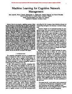
ROC curves (SNR= −8 dB, P = 1, L = 4, K = 128) (a) without noise power mismatch and (b) with noise power mismatch.
3.3
39
Misdetection probability versus P assuming (a) iid noise and (b) noniid noise.
3.2
38
Comparison of the different detectors. (a) Daher-Adve diversity order d. (b) Minimum operational SNR. . . . . . . . . . . . . . . . . . . .
3.1
37
. . . . .
64
66
Misdetection probability versus SNR for different detectors. Same scenario as in Fig. 3.2(b), with PFA = 0.01 and 0.1. . . . . . . . . . . xvii
67
xviii
LIST OF FIGURES
3.4
Distribution of the statistic −2 log T for L = 4 and K = 128. (a)
Under H0 (b) Under H1 . . . . . . . . . . . . . . . . . . . . . . . . . .
3.5
85
ROC curve showing the detection performance for OFDM and square root raised cosine signals when ρ = 0.15, L = 2 and K = 512. . . . .
87
3.6
PD performance versus SNR for fixed PF A = 0.05, L = 4 and K = 128. 88
4.1
False alarm and missed detection performance in a setting with M = 4 channels. (a) Test 1 (analytical). (b) Test 2 (analytical). (c) QGLRT (empirical). . . . . . . . . . . . . . . . . . . . . . . . . . . . . . . . . 117
4.2
Complementary ROC curves in a setting with M = 8 channels, for activity factor (a) a = 0.1 and (b) a = 0.9. . . . . . . . . . . . . . . . 118
4.3
Detector performance with frequency selective channels. . . . . . . . 119
4.4
Analytical performance of Test 2 as a function of the number of channels M . The sample size is given by K = 128M 2 . (a) Probability of misdetection. (b) Probability of false alarm. . . . . . . . . . . . . . . 120
4.5
Complementary ROC curves in a setting with M = 16 channels, K/N = 128/2048, for an activity factor (a) a = 0.1 and (b) a = 0.3.
4.6
128
Example of reconstruction of a mixed analog/digital broadcasting television band. . . . . . . . . . . . . . . . . . . . . . . . . . . . . . . 129
5.1
Secondary system 2-user rate region for different values of Q0 . . . . . 147
5.2
Primary/secondary users average performance in a time varying environment. (a) Primary user performance. (b) Secondary user performance. . . . . . . . . . . . . . . . . . . . . . . . . . . . . . . . . . 152
5.3
Primary user utility u0 for a fixed secondary interference I0 in a singleuser secondary system.
5.4
. . . . . . . . . . . . . . . . . . . . . . . . . 160
System behavior for identical secondary users when g(γ) = g (1) (γ). (a) Secondary utility. (b) Best-response functions. . . . . . . . . . . 161
5.5
System behavior for identical secondary users when g(γ) = g (2) (γ). (a) Secondary utility. (b) Best-response functions. . . . . . . . . . . 162
5.6
Game outcome assuming identical secondary users for a quasi-static scenario versus the number of secondary users K. . . . . . . . . . . . 163
LIST OF FIGURES
5.7
xix
System performance of the DSL game in quasi-static environments assuming identical secondary users. (a) Primary user utility. (b) Secondary user reward function.
5.8
. . . . . . . . . . . . . . . . . . . . 163
Game outcome in the presence for a quasi-static scenario versus the number of secondary users K. . . . . . . . . . . . . . . . . . . . . . . 164
5.9
System performance of the DSL game in quasi-static environments. (a) Primary user utility. (b) Secondary user reward function. . . . . 165
5.10 Outcome averaged over the fading for two different values of the weighting coefficient λs versus a growing channel variation rate �. (a) Game outcome. (b) Probability of undesired operation. . . . . . 168 5.11 Outcome averaged over the fading for two different values of the weighting coefficient λs versus a varying channel estimation period L. (a) Game outcome. (b) Probability of undesired operation. . . . . 169 5.12 Game outcomes averaged over fading for a quasi-static scenario and for time-varying scenario for a varying number of secondary users K. 170 5.13 System performance averaged over fading for a quasi-static scenario and for time-varying scenario. (a) Primary user utility. (c) Secondary reward function. . . . . . . . . . . . . . . . . . . . . . . . . . . . . . 170
Chapter 1
Introduction Contents 1.1
Cognitive Radio: Motivation
. . . . . . . . . . . . . . . .
1
1.2
Previous work . . . . . . . . . . . . . . . . . . . . . . . . .
2
1.3
1.1
1.2.1
Spectrum Monitoring . . . . . . . . . . . . . . . . . . . . .
3
1.2.2
Interference Management . . . . . . . . . . . . . . . . . . .
7
Contributions . . . . . . . . . . . . . . . . . . . . . . . . . .
7
1.3.1
Multiantenna and multichannel detection of primary users .
8
1.3.2
DSL: an Interference Management Scheme . . . . . . . . . . 10
1.4
Structure of the thesis . . . . . . . . . . . . . . . . . . . .
11
1.5
Notation . . . . . . . . . . . . . . . . . . . . . . . . . . . . .
11
Cognitive Radio: Motivation
In the recent years we have witnessed a constant increase in the price of the spectral resources. The main reason is the rising demand of spectrum as a result of emerging communication standards and services. However this scarcity of spectral resources happens while most of the allocated spectrum is underutilized. This paradox occurs only due to the inefficiency of traditional static spectrum allocation policies, which translates in a waste of spectral resources (FCC, 2002, 2003). Most of the useful spectrum is allocated to licensed users (e.g. mobile carriers, TV broadcasting companies) that do not transmit at all the geographical locations all the time. If this spectrum is opened for unlicensed use (e.g. private users, short range networks, ...) it is highly likely that a vast array
2
Chapter 1. Introduction
of new services will appear. One example of this is the huge innovation that has occurred in WiFi and Bluetooth operating in unlicensed bands, even though these two standards share just scraps of spectrum with many other technologies. The wireless industry has considerable interest in the development of dynamic spectrum access (DSA) as a means to improve spectral efficiency (FCC, 2002, 2003). Cognitive radio (CR) (Mitola and Maguire Jr., 1999) is receiving considerable attention as the enabling technology to achieve DSA in licensed bands. The key idea behind CR is to create smarter radios which are aware of, and can adapt to, their environment. Hence, in licensed bands CR nodes will monitor primary users in order to transmit in temporally and/or spatially unused slots. For example, the U.S. Federal Communications Commission (FCC) has recently issued a Second Report and Order (FCC, 2010), allowing operation on an unlicensed basis in the TV white spaces of VHF and UHF bands to both fixed and portable devices. While this order requires secondary users to access a database with information of the available resources, it is expected that these first steps start a major change to DSA in most of the spectrum once the CR technology is mature enough. One of the problems pointed out in FCC (2010) is that the available sensing technology is not reliable enough to guarantee that the interference produced to licensed (primary) users is kept at sufficiently low levels. Wireless propagation phenomena such as shadowing and fading pose significant challenges to the reliable detection of primary users. The received primary signal may be very weak, resulting in very low Signal-to-Noise Ratio (SNR) operation conditions and “hidden node” situations. Hence novel powerful spectrum monitoring techniques are required in order to increase CR network agility (Akyildiz et al., 2008). On the other hand, CR schemes may lead to very complex networks, in which primary and secondary users coexist in dynamic environments. This may lead to unexpected behavior and/or an impact on system performance. Hence, new schemes and analytical tools are required to control and model the interactions between the different elements of the system.
1.2
Previous work
While CR is a relatively novel area (Mitola’s landmark paper appeared in 1999 (Mitola and Maguire Jr., 1999)), it has received significant research interest in the last few years. In this section we present the most relevant previous work directly related
1.2 Previous work
3
to this thesis.
1.2.1
Spectrum Monitoring
Spectrum monitoring is based on the detection of weak signals from primary transmitters through the local observations of cognitive users, either individually or in a collaborative fashion. While cooperative sensing has the potential to overcome the effects of shadowing (Ganesan and Li, 2007a,b), it still relies on standalone detectors whose performance should be optimized. Three schemes are generally used for sequential individual sensing of primary channels, each of them requiring different degrees of knowledge and synchronization with the primary network: 1. Matched filter detection: If the secondary user is locked1 to the primary network, the optimal detection strategy in stationary Gaussian noise is matched filtering (Kay, 1998). Note that matched filter detection schemes require full synchronization with the primary network and thus they are difficult to implement in the low SNR conditions, which cognitive networks are expected to work in. 2. Feature based detection: Certain properties of the primary signal, such as the presence of any pilots or cyclostationary features, could in principle be exploited in order to obtain powerful detectors. However, such approaches become very sensitive to synchronization errors (Cabric, 2008). With very low SNR, the synchronization loops of the monitoring system cannot be expected to provide the required accuracy for the carrier frequency and/or clock rate estimates. 3. Asynchronous detectors: These detection schemes do not assume any synchronization with the primary signal. Hence they rely on other signal properties such as certain temporal and/or spatial structure. Among these, the most popular one is the energy detector, which does not require (or exploit) any a priori knowledge about the signal structure. The detector reduces to integrating received energy in a given frequency band and comparing it to a noise level dependent threshold. However, computation of the threshold in energy 1
Meaning that both frequency and timing synchronization loops are locked to a given set of signals.
4
Chapter 1. Introduction
detection requires knowledge of the noise variance. Any uncertainty regarding this parameter translates to severe performance degradation, so that the detection/false alarm requirements may not be satisfied (Tandra and Sahai, 2008). The reasons exposed motivate the search for asynchronous detectors robust to noise uncertainty, two possibilities being the use of multiple–antenna sensors and wideband monitoring covering multiple frequency channels. Moreover, if certain information about the primary network, such as channelization and modulation, is available to the spectrum monitor, it should be exploited to increase detection performance. In this thesis we will consider that this knowledge can be summarized as the spectrum shape / temporal correlation of the received signal. Several authors considered the problem of exploiting temporal structure of the received signal. Under the assumption that the power spectral density (psd) of the signal is completely known, Zhang et al. (2010b) derive the optimal Neyman-Pearson detector for both scalar and vector-valued signals. However, in spectrum sensing applications the propagation channel is unknown, and thus only partial knowledge of the second-order statistics is available in practice. A possible approach in that case is to neglect this partial knowledge, and consider test statistics that quantify the departure of the sample temporal autocorrelation matrix of the observations from the noise temporal covariance (Zeng and Liang, 2009a,b). Under the assumption that the signal is bandlimited, while its actual bandwidth, spectral shape and carrier frequency are unknown, Derakhtian et al. (2009) propose a generalized likelihood ratio test (GLRT) based scheme. Alternatively, metrics quantifying the distance of the sample correlation matrix from a “candidate” matrix summarizing a priori knowledge can be used: in the single–antenna setting, for example, Perez-Neira et al. (2009) assume the signal psd known up to a scaling and a shift, respectively modeling uncertainty about the power level and carrier frequency of the signal. Also assuming a single antenna, Quan et al. (2011) adopt a similar approach when the carrier frequency is known, as it often occurs in practice: for instance, for frequency division multiple access (FDMA) primary networks with public channelization parameters. However, all these works either assume that temporal correlation of the primary signal is unknown to the receiver or they do not consider the multiantenna and wideband settings.
1.2 Previous work
5
Multiantenna detection The gain offered by multiantenna processing in energy detection schemes was analyzed in Pandharipande and Linnartz (2007) under the assumption of channel information available to the secondary system. This assumption is not realistic in practice and the channel needs to be estimated. Assuming a temporally white Gaussian model for both signal and noise, spatially white noise with unknown (equal) variance across antennas, and an unknown spatial covariance matrix for the signal, several detectors have been proposed in the literature. We are particularly interested in the works based on the generalized likelihood ratio test (GLRT), since this approach usually results in simple detectors with good performance (Mardia et al., 1979). Under rank-1 spatial covariance for the signal and assuming iid noises, the GLRT is derived in Besson et al. (2006) and its application to CR was presented in Taherpour et al. (2010); Wang et al. (2010). When the signal covariance matrix is unstructured, and the noise assumed iid, the GLRT is the well-known test for sphericity (Mauchly, 1940), which was applied to CR in Lim et al. (2008); Zhang et al. (2010a). In these works the authors derived the GLRT for primary signals with spatial rank P > 1 under the assumption of iid noises with known variance. In Wilks (1935) the GLRT was derived for the case of an unstructured signal covariance matrix for non-iid noises. This detector was later applied to array signal processing in Leshem and Van der Veen (2001a,b). Other detectors which can handle different (unknown) noise variances have been proposed in Boonstra and Van der Veen (2003); Zeng and Liang (2009b). However, all of these works either assume rank-1 primary signals or unstructured primary signals. Moreover, they do not exploit any available information about the spectral shape of the primary signals. Once a multiantenna detector is proposed its performance must be evaluated. In order to quantify and compare the performance gain of multiantenna systems in fading environments, several metrics have been considered, including different concepts of detection diversity. One option is to adopt a definition analogous to the one from the communications literature for a certain performance tradeoff (between the probabilities of detection and false alarm), as proposed in Duan et al. (2010). A similar asymptotic definition based on J-divergence is given in Kim et al. (2009). In the context of radar, diversity order is however a low-SNR concept. For example, Daher and Adve (2010) define diversity order as the slope of the average probability of detection (P¯D ) curve with respect to the SNR at P¯D = 0.5.
6
Chapter 1. Introduction
Wideband detection In order to improve detection performance, the sensing system may also perform simultaneous acquisition of multiple frequency channels. This scheme improves the agility of the detector since multiple channels are processed at once and it provides the spectrum monitor with additional information to estimate the noise statistics as we will see in Chapter 4. This is mainly due to the availability of guard bands between adjacent channels, as well as to the fact that the presence of unused/weak channels within the subband can be exploited for noise variance estimation. Wideband spectrum sensing has been previously considered by several authors. In Hwang et al. (2010), knowledge of the noise variance is assumed, but the bandwidths and central frequencies of primary transmissions, as well as their number, are assumed unknown and estimated in turn. In the setting of Taherpour et al. (2008, 2009) primary system channelization is known, and the noise variance is regarded as unknown. However, these methods do not exploit a priori information about the psd of primary transmissions, and they assume that a minimum number of unused channels exist in the subband under examination. In a wideband setting, it may not be feasible to acquire the received signal at Nyquist rate. Novel sampling methods allow the reconstruction of the received signals from a set of compressed measurements if certain properties are met (Donoho, 2006). The key technology allowing this is compressive sensing, which is able to construct sparse solutions from a set of underdetermined equations. Several authors have applied compressed sensing to the detection of primary users in cognitive radio systems. Assuming a spectrum model consisting of several flat bandpass signals, and considering the edges between them, the observed signal is sparse in the “spectral edges domain”. This fact is used in Tian and Giannakis (2007) to propose a spectrum reconstruction algorithm from compressed samples of the signal autocorrelation estimate. This method was extended in Polo et al. (2009) in order to process directly a compressed version of the received signal (and not of its autocorrelation). These methods do not assume information about the primary network channelization, so that the spectral edges could occupy any position within the frequency band.
1.3 Contributions
1.2.2
7
Interference Management
In order to improve spectral efficiency, the wireless industry has prompted proposals for various dynamic spectrum access (DSA) approaches. A DSA scheme in which secondary users are allowed to opportunistically access the spectrum on the basis of no-interference to the primary (licensed) users, denoted as hierarchical access, is arguably the method that has received the most attention in recent literature. Various architectures have been proposed and investigated in recent years to achieve hierarchical dynamic sharing of licensed bands (see Kim et al. (2008); Le and Hossain (2008); Xing et al. (2007); Fattahi et al. (2007); Etkin et al. (2007); Menon et al. (2008) and references therein). A common assumption in these works is that the licensed users which own the spectrum rights are unaware of the presence of secondary users. Hence the burden of interference management relies mainly on the secondary system. In particular, either (i) there is a maximum interference level that the primary system is willing to tolerate, and the secondary powers/activity are to be adjusted within this constraint, or (ii) secondary users are allowed to opportunistically access the spectrum on the basis of no-interference to the primary (licensed) users. As opposed to this is the the concept of dynamic spectrum leasing (DSL), first presented in Jayaweera and Li (2009). A DSL scheme is characterized by the active role of the primary user, which may interact with the secondary system in order to define the allowed interference cap. This scheme allows the system to adapt to changing environmental conditions and may lead to a better spectral utilization.
1.3
Contributions
This thesis treats different aspects of a cognitive radio system. On the one hand, assuming a non-interfering DSA network we propose and analyze novel asynchronous multiantenna detectors and wideband detection schemes. Then, in the last chapter, we will study a DSA system in which certain interference is allowed at primary users, namely a DSL network.
8
Chapter 1. Introduction
1.3.1
Multiantenna and multichannel detection of primary users
In the previous section we showed the importance of deriving powerful asynchronous detectors for cognitive radio systems. To this end we need to exploit any available information about the primary network. In most of the analysis in this thesis we assume that the modulation / channelization of the primary network is known to the spectral monitor, which translates into a priori knowledge on the spectral shape of the primary transmissions. Additionally, we focus our study on Gaussian signals. The reasons for adopting a Gaussian model for the primary signal are as follows. First, under asynchronous sampling, the actual distribution is unknown; and since the noise is assumed Gaussian as well, the Gaussian pdf for the signal is the least informative one for the detection problem. Second, if the primary system uses multicarrier modulation with a sufficiently large number of subcarriers (which is the case in e.g. broadcasting applications), the Gaussian model is accurate (Tellado, 2000). Third, this model is tractable and leads to useful detectors under other distributions: note that Gaussianity is a common assumption in the development of signal detectors, either explicitly or implicitly, as many ad hoc methods that limit themselves to the use of second-order statistics of the observations can often be derived from a Gaussian model (the Energy Detector is the most prominent example). The main contributions of this thesis in spectrum monitoring are the following: • Derivation and analysis of different multiantenna detectors exploit-
ing a priori knowledge of the spectral shape of the primary transmissions when the noise statistics are assumed known. From the (non-implementable) Neyman-Pearson optimal detector we derive a family of practical multiantenna detectors with different levels of complexity. This will allow us to study both the advantages of exploiting spectral information and multiantenna processing under different scenarios.
• Diversity order analysis of multiantenna detection systems in cog-
nitive radio. In order to compare and rank the different detectors in fading environments we propose the use of two different performance metrics which reflect the diversity gain obtained by multiantenna systems. The first is analogous to the one used in communications and measures the asymptotic slope of the probability of misdetection with respect to the SNR (in log-log scale) for increasing SNRs. The second is borrowed from the radar community and
1.3 Contributions
9
is related to the behavior of the probability of detection around the point at which it equals 1/2. These key measures show the advantage of multiantenna processing when detecting primary signals. • Multiantenna detection of primary signals with spatial rank larger than one when the noise statistics are assumed unknown. Under the
Gaussian assumption, we derive the GLRT when both signal and noise are assumed temporally white and the primary signal may present an arbitrary spatial rank larger than one, both for spatially iid noises and when the noise is spatially uncorrelated but not necessarily iid. We emphasize the practical implications of this scenario. A primary signal with spatial rank larger than one will occur, for example, if multiple independent users (e.g. from adjacent cells) simultaneously access the same frequency channel. Alternatively, many state-of-the-art communication standards consider the simultaneous transmission of different data streams through multiple antennas to achieve multiplexing gain and/or the use of space-time codes to enhance spatial diversity. For these systems, the signal received at the multiantenna sensor will exhibit a spatial rank equal to the number of independent streams or the spatial size of the code, respectively. On the other hand, tolerances in the components of the analog frontends at different antennas will result in deviations of the noise level from antenna to antenna, and as it turns out, detectors derived under the iid assumption are very sensitive to these calibration errors. • Derivation and analysis of multiantenna detection of primary signals under strong interference. Assuming strong interference, modeled as temporally white noise with arbitrary spatial covariance matrix, we derive the GLRT for detection of primary signals with known temporal structure. We additionally propose a low SNR asymptotic analysis of this detector which can be tightened in the SNR range of interest. This analysis shows the existing tradeoff between the spectral shape of the primary signal and detection performance when the spatial structure of the signal is masked by the noise. This scenario may occur in the presence of strong cochannel interference generated by other secondary users. In this case, the secondary contributions can be modeled as noise with arbitrary and unknown spatial covariance. • Wideband detection in the presence of unknown noise level. Intu-
itively, if multiple primary channels are simultaneously acquired and channel-
10
Chapter 1. Introduction
ization information is available, the guard bands between adjacent channels could be used to estimate the noise power. We will show that when considering the problem of GLRT detection of one of the channels, not only the guard bands but also the empty/weak channels are used to improve the noise estimate. This analysis shows the advantages of performing wideband detection instead of channel-by-channel scanning. • Wideband detection from compressed measurements. We propose a primary user detection scheme from a set of compressed samples based on the
GLRT when the channelization of the primary network is assumed known. From a maximum a posteriori formulation we establish a connection between the estimation problem of the unknown parameters and certain compressed sensing techniques. Additionally, we propose a simple iterative procedure that conducts to similar detection performance as by using more complex convex optimization schemes.
1.3.2
DSL: an Interference Management Scheme
A DSL based paradigm allows certain amount of secondary interference at the primary system. Then primary user detection becomes less important in comparison to interference management. The main contribution in this section is the study of a family of DSL architectures showing their interference management capabilities. • Performance gain of DSL based paradigms. We present a theoretical analysis of the performance gain obtained by allowing a certain amount of interaction between primary and secondary systems. To this end, we define a family of performance metrics and propose a Stackelberg game formulation for the interactions between primary and secondary systems. We show that the performance gain obtained by allowing this interaction can be indeed large in dynamic environments. • Practical DSL scheme. Finally, we analyze certain practical DSL schemes which are shown to have a unique Nash equilibrium. In the stationary regime, the global performance of the system can be assumed to be the performance at the (unique) Nash equilibrium, which makes its analysis tractable. Moreover, the proposed DSL schemes show a graceful degradation under dynamic conditions and thus perform well in practice.
1.4 Structure of the thesis
1.4
11
Structure of the thesis
This thesis is divided in two different parts. In the first we address different spectrum monitoring schemes, focusing on multiantenna and wideband detectors. Then, in the second part, we propose a general framework for interference management in cognitive radio networks. In Chapter 2 we will study the problem of multiantenna detection exploiting a priori spectral information when the noise statistics are assumed known. In this chapter we will also pose the diversity order analysis of the proposed detectors. The case of multiantenna detection under unknown noise statistics will be covered in Chapter 3, including both the detection of primary signals with spatial rank larger than one, and detection in the presence of spatially unstructured noise. Chapter 4 covers the topic of wideband acquisition and detection, both when the band is acquired at Nyquist rate and when the detection must be performed from a set of compressed measurements. The analysis of a family of DSL schemes is presented in Chapter 5. Concluding remarks, as well as future lines of research, are included in Chapter 6.
1.5
Notation
Any non-standard notation used in this thesis is defined for the particular chapter at the point where the symbols first occur. For reader’s reference, we also include a comprehensive list of the notation in Table 1.1.
Symbol
Description
0 is the background noise power, assumed known and equal at all the antennas1 .
• The noise processes at different antennas are assumed statistically independent, i.e. E[nl nH n ] = IK 11(l = n).
By introducing the vectors
y1 . .. y= . , yL
n1 . .. n= . , nL
h1 . .. h= . , hL
(2.2)
the model (2.1) can be compactly written as y = h ⊗ s + σn.
(2.3)
Without loss of generality we assume E[|sk |2 ] = 1, since the signal power can be
absorbed into the channel vector h. Then, the average SNR per antenna is given by ||h||22 . E[||h ⊗ s||22 ] ζ= = . Lσ 2 E[||σn||22 ] 1
(2.4)
Since the noise variance is assumed known at each of the antennas, the derivation can be trivially extended to the case of different noise levels by rescaling the input signals so that all present noise variances equal to one.
16
Chapter 2. Calibrated Multiantenna Detection
Primary signal model In order to protect primary users from interference, the operational range of spectrum sensors must include primary signals well below decodability levels; in such situations, attempting to synchronize with the potentially present primary signal is unrealistic. Hence, we regard {sk } as a wide-sense stationary random process with
power spectral density (psd) Sss (eω ). We additionally adopt a Gaussian model for the primary signal. . Then we have that s ∼ CN (0, C), where C = E[ssH ]. Provided that the chan-
nelization and modulation parameters of the primary system are fixed and public (as would be the case, e.g., for broadcast networks), then Sss (eω ) is known (and so is C). Note that C is Toeplitz with ones on the diagonal. In general, {sk } will be colored (and C 6= I) as a result of interchannel guard bands, pulse shaping, etc.
In the sequel we will find useful the following asymptotic eigendecomposition of the primary signal temporal covariance matrix. Let C = UΛUH with Λ = diag(λ0 λ1 · · · λK−1 ) be an eigendecomposition of
C, and let W be the K ×K orthonormal IDFT matrix. As K → ∞ (long observation time) we have the following asymptotic result (Kay, 1998): λk → Sss (e
2πk K
),
0 ≤ k ≤ K − 1.
(2.5)
This result is based on the asymptotic equivalence of the sequences of matrices {C} and WΓWH }, where Γ = diag{Sss (1)Sss (e2π/K ) · · · Sss (e2π(K−1)/K )} for K = 1,
2,. . . (Gray, 2006), which has been exploited extensively in the literature; as shown in Zhang et al. (2010c), the loss in detection performance when adopting the approximation C ≈ WΛWH
(2.6)
often becomes negligible even for moderate values of K. The following spectral shape parameters will feature in the statistical analysis of the detectors: . 1 ¯bn = tr{Cn } = K ≈
K−1 1 X n λk K k=0 Z π 1 S n (eω )∂ω 2π −π ss
(2.7) for K → ∞.
(2.8)
2.3 Problem formulation
17
Note that ¯b1 = 1 since E[|sk |2 ] = 1. For white {sk }, C = I so that ¯bn = 1 for all n (in general, one has ¯bn ≥ 1 by Jensen’s inequality).
2.3
Problem formulation
The Neyman-Pearson lemma results in optimal detectors in the sense that the probability of detection is maximized for a given probability of false alarm (Kay, 1998). While in our setup the NP test is not implementable in practice it will lead to a series of practical detectors with a strong connection to the diversity combining techniques employed in communications (Simon and Alouini, 2004).
2.3.1
Neyman-Pearson detector
Based on the LK × 1 vector y from (2.3), and under the Gaussian model, the corresponding hypothesis test is given by H0 :
y ∼ CN (0, R0 )
(primary is absent)
(2.9)
H1 :
y ∼ CN (0, R1 )
(primary is present)
(2.10)
where we have introduced . R0 = σ 2 I, . R1 = σ 2 I + hhH ⊗ C,
(2.11) with
khk22
> 0.
(2.12)
This is a composite test (Kay, 1998), since h is unknown. Let now . G = hhH ⊗ C.
(2.13)
The NP test for this Gaussian detection problem is an estimator-correlator (Kay, ˆ exceeds a threshold, where z ˆ is the minimum mean 1998) declaring H1 true if yH z . squared error (MMSE) estimator of z = h ⊗ s given y and h. After some straightforward manipulations we obtain
ˆ = GR−1 z 1 y,
(2.14)
18
Chapter 2. Calibrated Multiantenna Detection
so that . ˆ TNP = yH z
(2.15)
= yH G(σ 2 I + G)−1 y
(2.16)
= yH (hhH ⊗ C)(σ 2 I + hhH ⊗ C)−1 y.
(2.17)
Note that this test cannot be directly implemented, since it requires knowledge of hhH . Single-antenna case At this point it is instructive to consider the single-antenna case. If L = 1, then G = |h|2 C, and the NP test statistic can be written as TNP =
X k∈B
|h|2 λk |vk |2 , σ 2 + |h|2 λk
(2.18)
. where v = [v0 v1 · · · vK−1 ]T = UH y, so that B ⊂ {0, 1, . . . , K − 1} is the set of indices of nonzero eigenvalues of C. In view of (2.5), for large K one has v ≈ WH y
(the DFT of the observations), and B is the support of Sss (eω ). In the following
asymptotic cases, the NP test becomes independent of |h|2 :
ˆ≈ • High SNR case: if |h|2 λk � σ 2 for all k ∈ B, then yH z
P
k∈B
|vk |2 . Thus the
NP test reduces to an Energy Detector (ED) over the spectral support of the ˆ ≈ vH v = yH y, i.e. the standard primary signal. If C is full rank, then yH z energy detector.
• Low SNR case: if |h|2 λk � σ 2 for all k ∈ B, then the NP test declares H1 true P if k∈B λk |vk |2 = yH Cy exceeds a threshold. This is also the Locally Most Powerful (LMP) test for this problem, derived from weak signal detection
theory (Kay, 1998). In contrast to the ED test, it makes use of the available information about the primary signal spectrum, since yH Cy can be interpreted 1/2
as the energy at the output of a filter with frequency response Sss (eω ) (a matched filter) fed by the observations y.
2.3 Problem formulation
2.3.2
19
Detection with multiple antennas
However, with L > 1 antennas, neither in the high nor low SNR regimes does the dependence of the NP test with hhH disappear. In the following we will focus in the case of asymptotically small SNR, of interest in Cognitive Radio systems. For asymptotically small SNR, if we make use of the first-order Taylor expansion R−1 1
≈
1 I, σ2
one has that the test TNP is proportional to . T0 = yH (hhH ⊗ C)y =
L X L X
hi h∗j yiH Cyj
(2.19) (2.20)
i=1 j=1
= gH Cg,
(2.21)
where we defined L
g = gMRC
. X ∗ = hl yl .
(2.22)
l=1
Here, as in the single-antenna case, T0 can be interpreted as the energy at the output of a matched filter, which now is fed by a linear combination g of the signals received at each of the antennas. We use the subscript MRC since this processing is akin to the Maximal Ratio Combining technique for multiantenna receivers (Simon and Alouini, 2004), by which the signals collected at each of the antennas are phasedaligned and combined with optimal weighting to maximize the SNR at the combiner output and prior to the demodulation stage. Note that the computation of the NP test statistic for low SNR does not require knowledge of the total channel gain, but . ¯= only of the spherical component h h/khk2 . The threshold can be set to achieve a given false alarm rate under H0 , i.e. under khk2 = 0. Now if we neglect the magnitude gains of the channel coefficients in (2.22), then g can be approximated as L
. X −θl yl g ≈ gEGC = e
(2.23)
l=1
. where θl = arg{hl }. In this case we correct the phase of the signals received at each
of the antennas before the linear combination. This is analogous to the Equal Gain Combining (EGC) technique in diversity reception.
20
Chapter 2. Calibrated Multiantenna Detection
The resemblance with different diversity combining techniques suggests a third detector based on Selection Combining (SC). In this case g is approximated by the signal at the branch with highest SNR: . g ≈ gSC = ym
with m = arg max |hi |2 .
(2.24)
1≤i≤L
Note that if the channel gains at all branches have similar magnitudes, then gEGC ≈ gMRC . On the other hand, when one of the channel gains is much larger than the remaining ones, then gSC ≈ gMRC .
However, as the reader should have noted, none of these three schemes (MRC, EGC and SC) is directly implementable, since they depend on unknown channel parameters. In order to avoid this problem, one option is to replace the unknown parameters by their corresponding estimates. Inspired by the Generalized Likelihood Ratio (GLR) approach, in Section 2.4 we present different scenarios in which the Maximum Likelihood (ML) estimates of the unknown parameters can be obtained; substituting these ML estimates in the corresponding statistics will in turn yield practical detectors. An alternative approach in order to handle the unknown parameters hi is to disregard antenna crosscorrelation and assume equal weighting for the energy estimates at the different antennas. In this case we obtain the following detector:
2.3.3
Generalized energy detector
By disregarding in T0 the cross terms depending on hi h∗j for i 6= j and assuming
|hi | ≈ |hj | for i 6= j, (2.20) reduces to TGED
L H1 1 X H = y Cy ≷ γGED , i i KLσ 2 H0
(2.25)
i=1
where the scaling factor (KLσ 2 )−1 was introduced for convenience and γGED is the decision threshold. We refer to this test as “Generalized Energy Detector” (GED), as it merely collects the (spectrally weighted) energy at all the branches. Notice that this detector is applicable to distributed settings with L collaborating single-antenna sensors: each node reports its local statistic yiH Cyi (scaled by the inverse of the local noise variance, if different nodes are affected by different noise levels) to a Fusion Center, where all such statistics are added together.
2.4 Parameter estimation and detection
21
The asymptotic performance of this detector is analyzed in Appendix 2.A.1, showing that for sufficiently large K and for a fixed threshold γGED , the probabilities of false alarm and detection are respectively given by !
PFA = Q
√
γGED − 1 KL p ¯b2
PD = Q
√
γGED − (1 + ζ ¯b2 ) KL p L¯b4 ζ 2 + 2¯b3 ζ + ¯b2
,
(2.26) ! .
(2.27)
Note that the performance of the GED test depends only on the average SNR ζ, ¯ of the channel vector. but not on the spherical component h
2.4
Parameter estimation and detection
In order to derive the low SNR ML estimates of the unknown parameters under the different models, we first obtain the likelihood function of the estimation problem. The log-likelihood function under H1 is log f (y | h) = − log det R1 −yH R−1 1 y, where
R1 depends on h as per (2.12). In the low SNR regime, using the fact that log(1 + x) ≈ x for small |x|, we can approximate
log det R1 ≈ KL log σ 2 +
tr G . σ2
(2.28)
On the other hand, R−1 1
� �−1 � � 1 1 1 1 = 2 I + 2G ≈ 2 I − 2G . σ σ σ σ
(2.29)
Thus, noting that tr G = tr hhH tr C = khk22 K, for low SNR one has log f (y | h) ≈ −KL log σ 2 −
2.4.1
Kkhk22 kyk2 yH Gy − 2 + . σ2 σ σ4
(2.30)
Selection Combining detector
The SC detector is based on the approximation (2.24), and thus requires the estimation of the index l of the antenna with largest SNR. ML estimation of this index in the general case is difficult, and thus we resort to the low SNR approximation (2.30); in addition, we will assume that h = hel , where el is the l-th unit vector. The rea-
22
Chapter 2. Calibrated Multiantenna Detection
son for this is that, as mentioned above, the SC approach is expected to provide close-to-optimal performance in scenarios in which the SNR at one of the antennas is dominant. Under this assumption, one has khk22 = |h|2 and yH Gy = |h|2 ylH Cyl in (2.30). Therefore, the ML estimate of l is just ˆl = arg maxl yH Cyl . The resulting decision l
rule is given by yH Cyl H1 . TSC = max l 2 ≷ γSC , 1≤l≤L Kσ H0
(2.31)
where the scaling factor (Kσ 2 )−1 does not affect the test. Thus, the SC detector picks the antenna with largest spectrally weighted energy and uses that energy as statistic. Note that this amounts to an OR fusion rule, applicable to distributed settings: the channel is declared busy if the spectrally weighted energy at any of the L nodes exceeds a threshold. In that case, only one bit of information has to be sent to the Fusion Center by each node, in contrast with the GED scheme. In Appendix 2.A.2 the asymptotic performance analysis of the SC detector is given. For large K and for a local threshold γSC , we obtain the global false alarm rate PFA = 1 −
1−Q
γ −1 pSC ¯b2 /K
!!L .
(2.32)
On the other hand, the probability of detection cannot be expressed in closed form, although it can be straightforwardly computed by means of a multivariate Gaussian integration routine; see Appendix 2.A.2. It must be noted that, in contrast with GED, the performance of the SC detector does depend on the spherical component of the channel vector.
2.4.2
Equal Gain Combining detector
For EGC detection, an estimate of the phases {θi }L i=1 introduced at the different
branches is needed in order to combine the respective signals as per (2.23). Considering again the low SNR approximation (2.30), it is seen that in order to obtain the ML estimates we must maximize the following quantity w.r.t. θ1 , . . . , θM : yH Gy =
L X L X n=1 m=1
|hn ||hm |ynH Cym e−(θm −θn ) .
(2.33)
2.4 Parameter estimation and detection
23
. Let anm = |hn ||hm |ynH Cym . Since anm = a∗mn , it is clear that yH Gy = ≤
L X
amm + 2
m=1 L X m=1
L L X X n=1 m=n+1
amm + 2
L L X X n=1 m=n+1
n. These constitute a set of L(L − 1)/2 (linear) conditions on our L free parameters, which in
general cannot be satisfied if L > 3. Nevertheless, careful inspection of the resulting P −θˆl y reveals that it is a function of the detection statistic gH Cg with g = L l l=1 e . ˆ ˆ ˆ phase differences θmn = θm − θn only. Thus, if we take these phase differences as our free optimization variables and neglect the dependence among them, the corresponding ML estimates are θˆmn = arg{ynH Cym }. This yields the following EGC
detection rule:
TEGC
. =
L L H1 1 XX H |y Cy | ≷ γEGC , n m KLσ 2 H0
(2.35)
n=1 m=1
which is intuitively satisfying: the lack of knowledge about the phase differences is sidestepped by considering the modulus of the crosscorrelation terms. Unfortunately, finding the distribution of TEGC (under either hypothesis) is intractable. An asymptotic Gaussian approximation is used in Appendix 2.A.3, showing that for large K for a given threshold γEGC ,
�
L−1 2
q
π¯b2 K
�
γEGC − 1 + √ , q PFA ≈ Q KL � 2L − 1 + (1 − L) π2 ¯b2 ! √ γEGC − (1 + κζ ¯b2 ) PD ≈ Q Kp ¯b4 (κζ)2 + 2¯b3 κζ + ¯b2
(2.36)
(2.37)
. ¯ 2 . Note that (2.37) is a function of the scaled average where κ = khk21 /khk22 = khk 1
SNR per antenna κζ, and that the scaling term κ ∈ [1, L] achieves its maximum
value when all elements of h have the same magnitude. Note that it is precisely in such scenarios that one expects the EGC detector to perform best.
24
Chapter 2. Calibrated Multiantenna Detection
2.4.3
Maximal Ratio Combining detector
For MRC detection, an estimate of the spherical component of the channel vector . ¯ = h/khk2 is needed. Let us introduce the data matrix Y = h [ y1 · · · yM ]. ¯ must Focusing again on the low SNR approximation (2.30), the ML estimate of h maximize yH Gy = yH (hhH ⊗ C)y = hH (YH CY)∗ h
¯ H (YH CY)∗ h. ¯ = khk22 h
(2.38)
¯ is the unit-norm eigenvector of (YH CY)∗ associated to This is achieved when h its largest eigenvalue (up to a phase term ejφ which does not affect the test). This results in the following scaled MRC detection rule: . λmax (YH CY) H1 TMRC = ≷ γMRC . Kσ 2 H0
(2.39)
Note that neither TEGC nor TMRC lend themselves to distributed implementation, since they require the computation of (spectrally weighted) crosscorrelations across the different antennas. The statistical analysis of the MRC detector amounts to finding the distribution of the largest eigenvalue of the random matrix YH CY under each hypothesis. For a general covariance matrix C, this remains an open problem. In Appendix 2.A.4 we present the analysis for a special case of practical interest: strictly bandlimited primary signals using a fraction B of the total channel bandwidth, and with flat psd within their passband. In this case, the distribution of TMRC under H0 asymptotically
follows a (shifted and scaled) Tracy-Widom distribution, which can be used to set the threshold γMRC for a given probability of false alarm. For fixed threshold γMRC the asymptotic probability of detection is given by � � 1 γMRC − δ1 + K(δLδ1 −1) √ ≈ Q δ1 / K
PDEGC . where δ1 = 1 + ¯b2 Lζ.
(2.40)
2.5 Detection diversity in fading environments
2.5
25
Detection diversity in fading environments
In the analysis of the previous section we considered that the SNR at each antenna is fixed. In practical conditions this is unlikely to occur. Consider a slow fading scenario in which the channel gains remain constant during the sensing window. Then h becomes a random variable and for a fixed threshold, the probability of detection PD is a random variable with expected value given by . ¯ = P¯D (ζ) Eζ {PD } =
Z
∞
fζ (ζ)PD (ζ) dζ,
(2.41)
0
. with fζ (ζ) the probability density function (pdf) of ζ, and ζ¯ = Eζ {ζ} the mean value of the SNR.
In the following we will assume that h can be modeled with a Ricean distribution (Simon and Alouini, 2004). This accounts for the line-of-sight (LOS) component and for the non-line-of-sight (NLOS) scattering. Hence at each realization we can model the channel vector as r � �r q η ¯ 1 ˜ 2 ¯ h = ζσ h+ h , 1+η 1+η
(2.42)
where ζ¯ denotes the average SNR and η stands for the Rice factor, the LOS channel . θ 2θ ¯ is defined as h ¯ = component h [e e · · · eLθ ] with θ ∼ U(0, 2π) modeling the ˜ is a zero-mean complex relative phase of the antennas of a uniform linear array, h Gaussian vector modeling the NLOS channel component with iid components ∼ CN (0, 1), and independent of θ.
The worst-case scenario in terms of detection performance is given by the NLOS channel, i.e. η = 0 with pure Rayleigh fading. We will see next that in this scenario the probability of misdetection (asymptotically) decreases only linearly with the SNR (in log scale) with a slope that is given by the asymptotic detection diversity of system. However, this asymptotic measure does not reflect the true detection performance of a detector in the SNR range of interest. To overcome this problem we will also present an analysis based on the diversity measure first proposed by Daher and Adve in the context of radar, related to the probability of detection around the SNR at which P¯D = 1/2.
26
Chapter 2. Calibrated Multiantenna Detection
2.5.1
High SNR diversity order analysis
We restrict here our analysis to the worst case given by iid Rayleigh fading scenarios2 , i.e. (2.42) with η = 0. In this case, the instantaneous SNR ζ = khk2 /(Lσ 2 ) is gamma-distributed (Simon and Alouini, 2004): fζ (ζ) =
LL ζ L−1 ¯ ζ > 0. exp {−Lζ/ζ}, (L − 1)! ζ¯L
(2.43)
We will next present the analysis for the GED. This analysis can be extrapolated with minor changes to the MRC detector. First, from (2.27), the probability of misdetection of the GED for a fixed threshold γGED is given by . PMD = 1 − PD ¯ (1 + ζ b2 ) − γGED = Q q . L¯b4 ζ 2 +2¯b3 ζ+¯b2 KL
(2.44) (2.45)
Using a first-order Taylor approximation of the argument of the Q-function in (2.44) about ζ = 0, one finds that in the low SNR regime,
PMD
i h ¯b2 + ¯¯b3 (1 − γGED ) (1 − γGED ) b p2 ≈ Q ζ+p . ¯b2 /KL ¯b2 /(KL)
(2.46)
In a fading environment, PMD in (2.46) becomes a random variable. Its mean value can be upper bounded by noting that 1 Q(x) ≤ e−x/2 , 2
x ≥ 0.
(2.47)
Note that this bound is looser than the more usual expression Q(x) ≤ e−x
2 /2
/2.
However, it will allow us to obtain a tight upper bound on the asymptotic slope of the probability of misdetection. By using this bound in (2.46) and then averaging 2
The analysis can be readily extended to Rayleigh fading with a certain correlation matrix Υ. The resulting asymptotic diversity will depend on the rank of Υ. We refer the interested reader to L´ opez-Valcarce et al. (2009).
2.5 Detection diversity in fading environments
27
. over h, the average probability of detection P¯MD = E[PMD ] can be bounded as P¯MD
) 1 − γGED p 2 b¯2 /(KL) ¯b2 + ¯¯b3 (1 − γGED ) . pb2 × E exp −ζ 2 b¯2 /(KL)
1 ≤ exp 2
(
(2.48)
Using similar steps to those in (Larsson and Stoica, 2003, Sec. 4.4), one finds that P¯MD ≤ CL ζ¯−L ,
(2.49)
where . 1 CL = exp 2
(
1−γ p GED 2 b¯2 /(KL)
)
2 ¯b2 +
p b¯2 L/K ¯b3 ¯b2 (1
− γGED )
L
(2.50)
is a constant independent of the average SNR. Hence the diversity order, that is, the slope of P¯MD versus the SNR when plotted on a log-log scale, is upper bounded by the number of antennas L of the receiver system. This shows the advantage of having multiple antennas for channel sensing under fading conditions even when considering the simple GED detector. By carrying a similar analysis, the MRC detector can be shown to present the same asymptotic diversity order in Rayleigh fading environments. Note that this analysis cannot be applied to EGC and SC detectors, since their performance depends on the actual SNR at each of the antennas and not on the global instantaneous SNR. If we define . 1 ζ = 2 [ |h1 |2 |h2 |2 · · · |hM |2 ]T , σ
(2.51)
so that ζ = [ζ1 · · · ζM ]T is the vector with the instantaneous SNR at each of the an-
tennas, an approximate analysis of the SC detector follows. The average probability of misdetection is in this case given by P¯MD =
Z fζ (ζ)PMD (ζ)∂ζ
(2.52)
where fζ (ζ) factorizes given the independent Rayleigh fading assumption. On the other hand, as it was shown in Appendix 2.A.2, PMD (ζ) does not factorize due to the present signal component. However, in low SNR conditions the correlation present
28
Chapter 2. Calibrated Multiantenna Detection
will be small and we may approximate P¯MD ≈
L �Z Y 0
l=1 ∞
�Z = 0
∞
(l) fζl (ζl )PMD (ζl )∂ζl
(1) fζ1 (ζ1 )PMD (ζ1 )∂ζ1
�
�L
(2.53) . = P˜MD
(2.54)
(l)
where PMD (ζl ) corresponds to the probability of misdetection of a single-antenna system with the instantaneous SNR given by ζl and in (2.54) we used the symmetry between antennas. Now, the misdetection probability at each of the antennas can be upper bounded using (2.49) with L = 1. Then one obtains the approximation P¯MD ≈ P˜MD ≤ C1L ζ¯−L ,
(2.55)
and, as a result, GED, MRC, and SC detectors cannot have a diversity order larger than L. In fact, as we will numerically show in Section 2.6 the diversity order bound is tight in the high SNR regime for the proposed detectors. Hence the four of them achieve full asymptotic diversity in uncorrelated Rayleigh fading.
2.5.2
Daher-Adve diversity order analysis
The asymptotic diversity order analysis presented in the previous section is a highSNR concept. However, spectrum sensors for CR systems are expected to provide high detection performance at much lower SNR values. This calls for a different definition of the diversity order better suited to the detection problem. In the context of radar processing, Daher and Adve (2010) define diversity order as the slope of the average probability of detection (P¯D ) curve with respect to the SNR at P¯D = 0.5. This notion of diversity is more adequate to CR networks because (i) it indicates a minimum operational SNR from which a detection scheme starts working reasonably well (i.e. P¯D ≥ 0.5) and (ii) describes how fast P¯D approaches 1 from this minimum operational SNR.
In this section, we characterize different spectrum sensing schemes in independent Rayleigh fading in terms of the Daher-Adve diversity order. As opposed to Daher and Adve (2010), in which the steering vectors are assumed known and a single snapshot is used per sensor for detection, when sensing on wireless channels,
2.5 Detection diversity in fading environments
29
the channel is not known and sensing times are longer in order to acquire several signal samples. Let the minimum operational SNR ζ¯∗ of the detector be defined by P¯D (ζ¯∗ ) = 0.5. Following Daher and Adve (2010), the diversity order d is defined as ¯ . ∂ P¯D (ζ) d= , ∂ ζ¯ ζ= ¯ ζ¯∗
with
1 P¯D (ζ¯∗ ) = . 2
(2.56)
. Unfortunately, P¯MD = E[PMD ] does not admit a closed-form solution for any of the detectors presented. In the high SNR asymptotic analysis we resorted to an upper bound of PMD which allowed us to obtain the analytical integral which is tight for high SNR. However, it is not possible to use a similar approach here since we are interested in intermediate SNRs. In order to obtain an approximation of the diversity order we propose the following first-order piecewise approximation of PMD (ζ), where ζ ∗ is such that PMD (ζ ∗ ) = 0.5:
PMD (ζ) ≈ . where ζ1 = ζ ∗ −
ζ=
ζ ∗,
i.e.
1 2a ,
. ζ2 = ζ ∗ +
1, 1 2
− a(ζ −
0 < ζ < ζ1 , ζ ∗ ),
ζ1 < ζ < ζ2 ,
0,
1 2a
(2.57)
ζ > ζ2 ,
and a is the negative of the slope of PM D (ζ) at
∂PMD (ζ) ∂PD (ζ) . a=− . ∗= ∂ζ ∂ζ ζ=ζ ∗ ζ=ζ
(2.58)
Using (2.43) and (2.57), one obtains P¯MD =
∞
Z
fζ (ζ)PMD (ζ) ∂ζ � � � � Lζ2 Lζ1 ≈ a ζ2 Γ , L − ζ1 Γ ,L ζ¯ ζ¯ � � � � ��� Lζ2 Lζ1 ¯ −ζ Γ ,L + 1 − Γ ,L + 1 ζ¯ ζ¯
(2.59)
0
�
(2.60)
where the incomplete Gamma function is defined as . Γ(x, α) =
1 Γ(α)
Z
x
tα−1 e−t ∂t,
0
. R∞ with Γ(α) = 0 tα−1 e−t ∂t denoting the standard Gamma function.
(2.61)
30
Chapter 2. Calibrated Multiantenna Detection
Taking derivatives in (2.59), and after some algebra, one arrives at the following approximation for the Daher-Adve diversity order � � ∗ � ∗ � �� ζ ζ 1 1 d ≈ a gL ¯∗ + ¯∗ − gL ¯∗ − ¯∗ , ζ 2aζ ζ 2aζ
(2.62)
. where gL (x) = Γ(Lx, L + 1). While (2.62) may look like a rough approximation of the diversity order, we will show in Section 2.6 that it effectively captures the behavior of P¯D in Rayleigh fading environments. We proceed now to compute the parameters ζ ∗ and a for the different detection schemes. GED detector performance Using the asymptotic distribution (2.27), one readily obtains the parameters ζ ∗ and a for the GED detector: 1 ∗ ζGED = ¯ (γGED − 1) , b r2 � �−1/2 ¯ ¯b3 KL¯b2 2 b4 L(γGED − 1) ¯3 + 2(γGED − 1) ¯2 + 1 aGED = , 2π b2 b2
(2.63) (2.64)
where we used that the derivative of the Q-function is given by 1 ∂Q(x) = √ exp (−x2 ). ∂x 2π
(2.65)
Now, finding the value of ζ¯∗ at which (2.59) equals 0.5 is not straightforward. ∗ However, an obvious candidate is ζ¯∗ ≈ ζGED , since the instantaneous probability of . ∗ misdetection satisfies PMD (ζGED ) = 0.5. With �GED = 2aGED1 ζ ∗ , this yields GED
dGED ≈ aGED [gL (1 + �GED ) − gL (1 − �GED )] ,
(2.66)
∗ where both aGED and ζGED depend on the system parameters K, L, ¯bi and PFA .
Noting that the bracketed term in (2.66) is less than 1, the following upper bound is obtained:
r dGED < aGED
0, we have that3 gL (1+�) → 1 whereas gL (1−�) → 0. 3
Intermediate steps can be found in Appendix 2.B.
2.5 Detection diversity in fading environments
31
Thus, for large L, dGED ≈ aGED . Remark 2.1. From (2.67), Daher-Adve diversity order of the�GED detector under � p uncorrelated Rayleigh fading is asymptotically bounded by O KL¯b2 . Moreover, ∗ for small values of ζ¯ this bound becomes asymptotically tight, i.e. for a small minimum operational SNR, dGED grows with the square root of the number of antennas L multiplied by the parameter ¯b2 = tr{C2 }/K. Since ¯b2 ≥ 1 with equality for
temporally white primary signals, we have that Daher-Adve diversity increases with the temporal correlation of the primary signals. Moreover, for larger values of ¯b2 we attain a lower minimum operational SNR (2.63), hence increasing the operational range of the detector. MRC detection performance In this case, the parameters for the first-order piecewise approximation of (2.40) are � p 1 � ∗ ζMRC = ¯ β + (2 + β)2 − 4γMRC , 2b2 L r L KL2¯b22 1 − K(¯b2 Lζ)2 aMRC = , 2π 1 + ¯b2 Lζ where β = γMRC −
K+L K ,
(2.68) (2.69)
so that r dMRC < aMRC
1, the advantage of the iterative scheme alterntng-GLRT over the asymptotic GLRT decreases. This can be explained from the fact that, as the total SNR is divided among a growing number of dimensions, the effective SNR per dimension decreases and one gets closer to the asymptotic regime for which asympt-GLRT was derived. Noise mismatch effect on detection performance We now investigate the effect of a noise level mismatch at the different antennas on the different detectors. In order to focus on this effect we fix P = 1. Figure 3.2 shows the corresponding receiver operating characteristic (ROC) curves in a scenario with iid noises and with non-iid noises. In Fig. 3.2(a) we can see that for an scenario with iid noises (noise powers at each antenna equal to 0 dB) the iidGLRT test, corresponding to the GLRT under this model, yields the best detection performance, whereas the detectors designed for disparate noise variances suffer a noticeable penalty. From the detectors designed for uncalibrated receivers, it is seen that the GLRT based schemes, both asymptotic and iterative, behave similarly and outperform the Hadamard ratio detector. The heuristic detector based on statistical covariances (Zeng and Liang, 2009b) presents almost the same performance as
Chapter 3. Multiantenna Detection under Unknown Noise Statistics
1
1
0.9
0.9
0.8
0.7
iid-GLRT Sphericity alterntng-GLRT Lim et al. asympt-GLRT Hadamard Covariance
0.6
0.5 0
0.1 0.2 0.3 0.4 False Alarm Probability
(a)
0.5
Detection Probability
Detection Probability
66
0.8
0.7
iid-GLRT Sphericity alterntng-GLRT Lim et al. asympt-GLRT Hadamard Covariance
0.6
0.5 0
0.1 0.2 0.3 0.4 False Alarm Probability
0.5
(b)
Figure 3.2: ROC curves (SNR= −8 dB, P = 1, L = 4, K = 128) (a) without noise power mismatch and (b) with noise power mismatch. the Hadamard ratio test, while the detector of (Lim et al., 2008) suffers a penalty compared to the GLRT for the same model. Fig. 3.2(b) shows the ROC curves for a similar scenario, but with different noise variances across the antennas, now given by 0, −1, 1.5 and −0.5 dB. Note that the performance of the detectors designed for uncalibrated receivers has not changed with respect to that in Fig. 3.2(a), whereas that of the detectors based on the iid noise assumption is severely degraded. Asymptotic GLRT performance for finite SNR values Although the asymptotic GLRT detector (asympt-GLRT ) given by (3.34) is appealing due to its computational simplicity, it is not clear how much can be gained when the iterative scheme (alterntng-GLRT ) is used in order to implement the exact GLRT. Fig. 3.3 shows the missed detection probability of the detectors versus the SNR in a scenario similar to that of the previous subsection (P = 1, L = 4, K = 128, different noise levels at each of the antennas fixed to 0, −1, 1.5 and −0.5
dB respectively). The probability of false alarm is fixed to PFA = 0.01 and 0.1. In Fig. 3.3 it is seen that, as expected, for very low SNR values the asymptotic detector presents the same performance as the alternating minimization scheme. However, as the SNR increases, the GLRT outperforms the detector derived for asymptotically
3.4 Detection of rank-1 signals in spatially correlated noise
Misdetection Probability
10
10
10
67
0
PF A = 0.01 PF A = 0.1
−1
−2
−3
10 −10
Hadamard asympt-GLRT alterntng-GLRT −9
−8
−7 −6 −5 Average SNR [dBs]
−4
−3
−2
Figure 3.3: Misdetection probability versus SNR for different detectors. Same scenario as in Fig. 3.2(b), with PFA = 0.01 and 0.1.
low SNR, as it could be expected. Note, however, that the performance loss of the asymptotic detector is rather small, and therefore it offers a good tradeoff between performance and complexity.
3.4
Detection of rank-1 signals in spatially correlated noise
In the previous section we assumed the noise process uncorrelated across antennas. While this accurately models the thermal noise effects, other contributions such as cochannel interference will present spatial correlation. In this section no assumptions are made about Σ2 other than to have full rank. Under the Gaussianity assumption, if we do not impose any constraint on the the spatial covariance of the noise process, we must resort to additional information (other than spatial) in order to detect the primary signal. To this end, in this section, we assume that the primary signal presents certain temporal correlation which translates into C 6= IK . The matrix C is assumed to be available to the spectral monitor as a priori information. In this section we will restrict our study
to primary signals of rank one, thus, H = hH with h an L × 1 vector and S = s is
68
Chapter 3. Multiantenna Detection under Unknown Noise Statistics
K × 1. Then we have that the received signal reduces to Y = shH + NG.
(3.40)
In the following we will find useful to define the maximum achievable SNR as . ρ = hH Σ−2 h = khΣ k22 ,
(3.41)
where the prewhitened channel is given by . hΣ = Σ−1 h.
(3.42)
Note that ρ = hH Σ−2 h is the maximum SNR that can be obtained at the output of a linear combiner (beamformer), i.e. if we let x = Yv = shH v + NGv with v the L × 1 beamformer, then the SNR of x is given by . ζ=
E[vH hsH shH v] vH hhH v , = E[vH GH NH NGv] vH Σ2 v
(3.43)
which attains its maximum value ζ = hH Σ−2 h for v = Σ−2 h. As in the previous section h and Σ2 = GH G are modeled as deterministic and unknown. However, as a preliminary step before the derivation of the GLRT for this problem, we study the optimal detector assuming a priori knowledge of h and Σ2 .
3.4.1
Genie-aided detectors
If h and Σ2 are assumed known the optimal detector is given by the Neyman-Pearson test. Let us consider the whitened received signal, defined as . yΣ = (Σ−T ⊗ I) y,
(3.44)
as the new input to the detector. It is easy to see that in this case the system model corresponds to the one considered in Chapter 2 when σ 2 = 1. Hence, following similar steps the optimal NP test can be found to be � �� �−1 H T H T TNP = yΣ yΣ (hΣ hH Σ ) ⊗ C ILK + (hΣ hΣ ) ⊗ C
(3.45)
where we have defined the whitened channel as hΣ = Σ−1 h. Using the definition of the Kronecker product and the Matrix Inversion Lemma, we have that the inverse
3.4 Detection of rank-1 signals in spatially correlated noise
69
T −1 can be rewritten as3 [ILK + (hΣ hH Σ ) ⊗ C] T −1 T [ILK + (hΣ hH = ILK − (hΣ hH Σ ) ⊗ C] Σ ) ⊗ C(ρ),
(3.46)
where we defined . C(ρ) = C1/2 (IK + ρC)−1 C1/2 .
(3.47)
Note that C(0) = C, whereas C(ρ) ≈ 1/ρIK for ρ → ∞. Applying this result to (3.45) we obtain
� H T TNP = yΣ (hΣ hH Σ) � H T = yΣ (hΣ hH Σ) � H T = yΣ (hΣ hH Σ) � H T = yΣ (hΣ hH Σ) � H T = yΣ (hΣ hH Σ)
�� � T ⊗ C ILK − (hΣ hH Σ ) ⊗ C(ρ) yΣ � H T ⊗ C − (hΣ hH Σ hΣ hΣ ) ⊗ (CC(ρ)) yΣ � T ⊗ C − (hΣ hH Σ ) ⊗ (ρCC(ρ)) yΣ � ⊗ (C(IK − ρC(ρ))) yΣ �� ⊗ C(IK + ρC)−1 yΣ
(3.48) (3.49) (3.50) (3.51) (3.52)
H −2 where in (3.50) we have used that hH Σ hΣ = h Σ h = ρ and in (3.52) we made use
of the identity IK − ρC(ρ) = (IK + ρC)−1 . We now apply the property tr(AT BH CD) = vec(B)H (A ⊗ C) vec(D)
(3.53)
in (3.52) to obtain, after some straighforward manipulations, H −1 TNP = hH Σ YΣ C(IK + ρC) YΣ hΣ
= hH Σ−2 YH C(IK + ρC)−1 YΣ−2 h
(3.54) (3.55)
. where we have defined YΣ = vec(yΣ ) = YΣ−1 . Note that v = Σ−2 h corresponds to the optimum beamformer, which maximizes the SNR at its output x = Yv. Then the NP test can be written as TNP = xH C(IK + ρC)−1 x ≈ xH WΛ(IK + ρΛ)−1 WH x,
(3.56) (3.57)
where have made use of the asymptotic EVD of the covariance matrix C ≈ WΛWH , 3
Intermediate steps can be found in Appendix 3.B.
70
Chapter 3. Multiantenna Detection under Unknown Noise Statistics
first introduced in (2.5). By examining (3.57) the structure of the NP test becomes clear. First, the received signal is fed through the optimal spatial beamformer x = Yv. This signal is then transformed into the frequency domain by applying the FFT transform WH and fed through the optimal Wiener filter ω
F (e ) =
�
Sss (eω ) 1 + ρSss (eω )
�1/2 ,
(3.58)
before the energy of the resulting signal is compared against a threshold. That is, the optimal NP detector relies on two key components. The first is the optimum beamformer v which maximizes the received SNR by discarding the noise-only spatial dimensions. In second place we have an optimum Wiener filter which acts as a matched filter in the temporal domain. At this point it is instructive to consider the following asymptotic cases, in which the structure of this filter simplifies: • In the high SNR regime, ρ → ∞, i.e., F (eω ) → ρ−1/2 and the detector amounts
to comparing the energy at the output of the optimum beamformer kxk2 =
xH x with a given threshold.
• In the low SNR regime, ρ → 0, so that C(IK + ρC)−1 → C, and the test reduces to comparing xH Cx against a threshold.
However, neither h nor Σ2 can be assumed known and need to be estimated. The ML estimation of these parameters under both Hypothesis conducts to the GLRT detector.
3.4.2
GLRT detector
We now proceed to the derivation of the GLRT based on (3.40), as presented in (3.9). ML parameter estimation under H0 Under H0 the signal covariance is given by R0 = (Σ2 )T ⊗ IK where Σ2 is unstruc-
tured.
Lemma 3.5. Under H0 , the ML estimate of the (unstructured) noise covariance matrix is given by
ˆ2 = R ˆ = 1 YH Y. Σ K
(3.59)
3.4 Detection of rank-1 signals in spatially correlated noise
71
Proof. Under H0 the log-likelihood reduces to � � ˆ −2 , log f (Y | Σ) = −LK log π − K log det(Σ2 ) − K tr RΣ
(3.60)
ˆ (Magnus and Neudecker, 1999). which is maximized for Σ2 = R ML parameter estimation under H1 Under H1 , the log-likelihood is given by log f (y | R1 ) = −LK log π − log det(R1 ) − yH R−1 1 y,
(3.61)
R1 = (Σ2 )T ⊗ IK + (hhH )T ⊗ C.
(3.62)
with
Note that (3.61) offers little information about the ML estimates of Σ2 and h. However, from the structure of R1 in (3.62) it is apparent that spatial and temporal correlations are separable in terms of the Kronecker product. Using this fact, we derive next a simpler expression for (3.61) which will allow us to reduce the optimization problem in Σ2 and h to a scalar optimization problem. First, the inverse of R1 can be written as � �−1 R1−1 = (Σ2 )T ⊗ IK + (hhH )T ⊗ C � � � �−1 � −1 T � = (Σ−1 )T ⊗ IK ILK + (Σ−1 hhH Σ−1 )T ⊗ C (Σ ) ⊗ IK −2 T
= (Σ
−2
) ⊗ IK − (Σ
H
−2 T
hh Σ
) ⊗ C(ρ)
(3.63) (3.64) (3.65)
where in the last step we used (3.46). Now applying the property (3.53) some straightforward algebra yields −2 H −2 H −2 H yH R−1 1 y = tr{Σ Y Y − Σ hh Σ Y C(ρ)Y}.
(3.66)
On the other hand, using a generalization of Sylvester’s determinant identity4 4
det(A + UVH ) = det(A) det(I + VH A−1 U).
72
Chapter 3. Multiantenna Detection under Unknown Noise Statistics
to Kronecker products, we can rewrite the determinant term in (3.61) as � log det(R1 ) = log det (Σ2 )T ⊗ IK + (hhH )T ⊗ C = K log det(Σ2 ) + log det(IK + ρC).
(3.67) (3.68)
Substituting (3.68) and (3.66) into the log-likelihood (3.61) yields log f (y | hΣ , Σ) = −LK log π − K log det Σ2 − log det(IK + ρC) � � −1 H −1 − tr Σ−2 YH Y + tr hΣ hH . (3.69) Σ Σ Y C(ρ)YΣ Defining a new parameter space In order to maximize (3.69) we will find useful to replace the parameter space {hΣ , Σ−2 } by a more convenient form. First, using the following identity: IK − ρC(ρ) = (IK + ρC)−1 , we may reorganize the terms in (3.69) to obtain
¯ Σ , Σ−2 ) = −LK log π − K log det Σ2 − log det(IK + ρC) log f (y | ρ, h � � � ¯ Σh ¯ H Σ−1 YH YΣ−1 − tr h ¯ Σh ¯ H Σ−1 YH (IK + ρC)−1 YΣ−1 . − tr IL − h Σ Σ
(3.70)
. ¯Σ = where we have introduced the unit-norm vector h hΣ /khΣ k2 . This step is important in what follows because it divides the spatial contribution of the prewhitened received signal YΣ−1 in two different terms: one orthogonal and one collinear to the prewhitened channel hΣ , respectively. We now define the two quasi-orthogonal contributions to the inverse of the spatial covariance matrix of the noise Σ−2 = W⊥ + Wk as � . ¯ Σh ¯ H Σ−1 = U⊥ ∆⊥ UH , W⊥ = Σ−1 IL − h Σ ⊥ . −1 ¯ ¯ H −1 H Wk = Σ hΣ hΣ Σ = δk uk uk ,
(3.71) (3.72)
where U⊥ ∆⊥ UH ⊥ denotes the economy-size eigendecomposition of the matrix W⊥ (of rank L − 1), and the economy-size eigendecomposition of the rank-1 matrix Wk is given by δk uk uH k . Then we have the following result:
Lemma 3.6. The log-likelihood (3.70) can be rewritten in terms of a new parameter
3.4 Detection of rank-1 signals in spatially correlated noise
73
¯ ρ, U⊥ , ∆⊥ , uk , δk } as space given by {h, ¯ δk , uk , ∆⊥ , U⊥ ) = log f (y | ρ, h,
¯ H uk |2 − log det(IK + ρC) − LK log π + K log det ∆⊥ + K log δk + K log |h
−1 H H H − tr{U⊥ ∆⊥ UH ⊥ Y Y} − tr{δk uk uk Y (IK + ρC) Y}, (3.73)
. ¯= with h h/khk2 . Proof. We have that U⊥ is an L × (L − 1) semiunitary matrix. Its nullspace is given ¯ since by the direction h � ¯ = Σ−1 IL − h ¯ Σh ¯ H Σ−1 h ¯ W⊥ h Σ � � H h −2 −2 −2 hh = Σ −Σ −2 Σ H khk2 h Σ h � −2 � H 1 h Σ h = 0. = Σ−2 h − Σ−2 h H −2 khk2 h Σ h
(3.74) (3.75) (3.76)
¯ defines a unitary matrix and the full eigenvalue decomposition As a result [U⊥ h] ¯∆ ¯ H , where we defined ˜ ⊥ [U⊥ h] of W⊥ is given by W⊥ = [U⊥ h] . ˜⊥ = ∆
"
#
∆⊥ 0
.
(3.77)
Now, the determinant of Σ−2 can be rewritten as det Σ−2 = det(W⊥ + Wk ) � � ¯∆ ¯ H + uk δk uH ˜ ⊥ [U⊥ h] = det [U⊥ h] k � � ¯ ¯ H uk δk uH [U⊥ h] ˜ ⊥ + [U⊥ h] = det ∆ k
(3.78) (3.79) (3.80)
¯ adj(∆ ¯ H uk ˜ ⊥ ) + δk uH [U⊥ h] ˜ ⊥ ) [U⊥ h] = det(∆ k
(3.81)
T ¯ ¯H = δk uH k [U⊥ h] [eL det(∆⊥ )eL ] [U⊥ h] uk
(3.82)
¯ ¯H = δk uH k h det(∆⊥ ) h uk
(3.83)
¯ H uk |2 det(∆⊥ ), = δk |h
(3.84)
where in (3.81) we have used that (see e.g. (Lancaster and Tismenetsky, 1985, p. 65)) det(X +yz T ) = det(X)+z T adj(X)y where adj(·) denotes the adjugate matrix, ˜ ⊥ ) = 0 and that the adjugate matrix of a and in (3.82) we have used that det(∆
74
Chapter 3. Multiantenna Detection under Unknown Noise Statistics
diagonal matrix with the i-th diagonal entry equal to zero, is the zero matrix except for the (i,i)-th component. Substituting (3.71), (3.72), (3.84) in the likelihood expression given in (3.70) we obtain the desired result. ¯ Σ , Σ−2 }, we exThat is, in order to maximize (3.70) with respect to {ρ, h
pressed the log-likelihood in terms of an alternative set of parameters, namely ¯ ρ, U⊥ , ∆⊥ , uk , δk }. Note that the number of degrees of freedom of the two sets {h, of parameters is the same. The first set of parameters presents L2 degrees of free¯ Σ and 1 in the dom in the Hermitian matrix Σ−2 , 2L − 1 in the unitary vector h
effective SNR ρ, that is, a total of L2 + 2L degrees of freedom. On the other hand, ¯ defines an unitary matrix with L2 − L degrees of freedom, {uk , δk } define [U⊥ h] a complex vector with 2L degrees of freedom, and ∆⊥ and ρ present L − 1 and 1 degrees of freedom respectively, adding up to a total of L2 + 2L degrees of freedom.
Additionally, it is possible to establish a biunivocal mapping between the two sets ¯ Σ , the matrices W⊥ and Wk can be computed using of parameters. Given Σ−2 , h ¯ Σ as (3.71)-(3.72), and viceversa, given W⊥ , Wk , we may compute Σ−2 , h Σ−2 = W⊥ + Wk ,
¯Σ = h
Σuk . kΣuk k2
(3.85)
Hence, the maximization can be carried out over the new set of parameters given ¯ ρ, U⊥ , ∆⊥ , uk , δk }. by {h, Compressing the log-likelihood We must now maximize the log-likelihood with respect to the unknown parameters. Let us define to this end the “orthogonal component” of the observations as . ¯h ¯ H )YH Y(IL − h ¯h ¯ H ). (YH Y)⊥ = (IL − h
(3.86)
¯ = 0. It then ¯ = 0, which in turn implies that U⊥ h We recall from (3.76) that W⊥ h H H H follows that UH ⊥ Y YU⊥ = U⊥ (Y Y)⊥ U⊥ . Consider now an economy-size EVD
of the rank-(L − 1) matrix (YH Y)⊥ : (YH Y)⊥ = UY⊥ ∆Y⊥ UH Y⊥ .
(3.87)
3.4 Detection of rank-1 signals in spatially correlated noise
75
¯ = 0, and therefore UY⊥ h ¯ = 0. Since both U⊥ , UY⊥ are Observe that (YH Y)⊥ h L × (L − 1) matrices with orthonormal columns, and both of them are orthogonal to ¯ it follows that U⊥ , UY⊥ span the same subspace. Hence, there the same vector h, must exist an (L − 1) × (L − 1) unitary matrix UΩ such that U⊥ = UY⊥ UΩ .
(3.88)
Using the definition of UΩ in (3.88), the log-likelihood function can be written as ¯ uk , δk , ∆⊥ , UΩ ) = log f (y | ρ, h,
¯ H uk |2 − log det(IK + ρC) − LK log π + K log det ∆⊥ + K log δk + K log |h
H −1 − tr{UΩ ∆⊥ UΩ ∆Y⊥ } − δk uH k Y (IK + ρC) Yuk . (3.89)
The only term depending on UΩ is − tr{UΩ ∆⊥ UΩ ∆Y⊥ }. For the diagonal el-
ements of ∆Y⊥ sorted in non-increasing order and the diagonal elements of ∆⊥
sorted in non-decreasing order (to be checked later) the term − tr{UΩ ∆⊥ UΩ ∆Y⊥ }
is maximized with respect to UΩ for (Fraikin et al., 2008) ˆ Ω = IL−1 . U
(3.90)
ˆ ⊥ is straightforward and Now, the maximization of (3.89) with respect to δk and ∆ yields H −1 −1 δˆk = K(uH k Y (IK + ρC) Yuk ) ,
ˆ ⊥ = K∆−1 . ∆ Y⊥
(3.91) (3.92)
Note that indeed since the diagonal elements of ∆Y⊥ are sorted in non-increasing order, the diagonal elements of ∆⊥ are sorted in non-decreasing order. Hence the assumption in obtaining (3.90) was right. Substituting (3.90), (3.91) and (3.92) into (3.89), we obtain the compressed log-likelihood function ¯ uk ) = −LK log π + LK log K − LK + K log |h ¯ H uk |2 log f (y | ρ, h, h i H −1 − log det(IK + ρC) − K log uH k Y (IK + ρC) Yuk − K log det(∆Y⊥ ). (3.93) In order to proceed now, the following result will be useful. Lemma 3.7. Let A be an L × L invertible matrix, and let G be an unitary matrix
76
Chapter 3. Multiantenna Detection under Unknown Noise Statistics
partitioned as G = [g1 G⊥ ] where g1 is L × 1 and G⊥ is L × (L − 1). Then it holds
that
H −1 det(GH ⊥ AG⊥ ) = g1 A g1 det(A).
(3.94)
Proof. The proof can be found in Appendix 3.C. Observe that, since UH Y⊥ UY⊥ = IL−1 , one has H ∆Y⊥ = UH Y⊥ (Y Y)⊥ UY⊥ H = UH Y⊥ (Y Y)UY⊥ ,
(3.95) (3.96)
¯ = 0. Since the matrix where the second step follows from the fact that UY⊥ h ¯ UY⊥ ] is unitary, we can apply the result from Lemma 3.7 to obtain [h ¯ det(YH Y). ¯ H (YH Y)−1 h) det(∆Y⊥ ) = (h
(3.97)
Therefore, the log-likelihood (3.93) reads as ¯ uk ) = log f (y | ρ, h,
¯ H uk |2 − log det(IK + ρC) −LK log π + LK log K − LK + K log |h h i � H H −1 � H −1 H ¯ ¯ − K log uH k Y (IK + ρC) Yuk − K log h (Y Y) h − K log det(Y Y). (3.98) ¯ and uk amounts to minimizing Maximizing (3.98) with respect to h ¯ H (YH Y)−1 hu ¯ H YH (IK + ρC)−1 Yuk h k . ¯ H uk |2 |h
(3.99)
To this end, we can apply the following result: Lemma 3.8. Let A1 and A2 be two L × L Hermitian matrices, and let . uH A1 u1 uH 2 A2 u2 J(u1 , u2 ) = 1 . H |u1 u2 |2
(3.100)
The minimum of J is given by the smallest eigenvalue of the matrix A1 A2 (which
3.4 Detection of rank-1 signals in spatially correlated noise
77
is also the smallest eigenvalue of A2 A1 ), and it is attained, when u?1 /c1 = eigenvector of A2 A1 associated to its smallest eigenvalue,
(3.101)
u?2 /c2 = eigenvector of A1 A2 associated to its smallest eigenvalue,
(3.102)
with c1 and c2 two arbitrary nonzero complex scalars. Proof. The proof can be found in Appendix 3.D. Therefore, the optimum value of (3.99) is given by � . χ = λmin (YH (IK + ρC)−1 Y)(YH Y)−1 ,
(3.103)
¯ and uk , up to a complex scaling factor, are respecwhereas the ML estimates of h tively given by ˆ¯ = eigenvector of (YH (I + ρC)−1 Y)(YH Y)−1 associated to λ , h min K H
−1
ˆ k = eigenvector of (Y Y) u
H
(Y (IK + ρC)
−1
Y) associated to λmin ,
(3.104) (3.105)
where with some abuse of notation we used λmin to denote the smallest eigenvalue of the corresponding matrix. Consider now the singular value decomposition (SVD) of the data matrix H Y = UY SY VY
(3.106)
where UY is K × L with orthonormal columns; SY is L × L diagonal, with the singular values of Y; and VY is L × L unitary. Then, it is easily seen that χ can be written as
� −1 χ = λmin UH Y (IK + ρC) UY .
(3.107)
With this, the compressed log-likelihood under H1 can be finally written as π . `1 = −LK(1 + log ) − K log det YH Y K � H −1 H −1 � λ−1 min (Y (IK + ρC) Y)(Y Y) + K max log , ρ≥0 det1/K (IK + ρC) which must be maximized only over the scalar parameter ρ.
(3.108)
78
Chapter 3. Multiantenna Detection under Unknown Noise Statistics
GLRT detector From Lemma 3.5 the compressed log-likelihood under the hypothesis 0 is given by `0 = max log f (y | R0 )
(3.109)
= −LK(1 + log
(3.110)
Σ2
π ) − K log det (YH Y). K
Therefore, the GLRT statistic (3.9) is found to be `1 −`0
T =e
� H −1 λ−K min UY (IK + ρC) UY , = max ρ≥0 det(IK + ρC)
(3.111)
whose computation involves a maximization with respect to a scalar parameter only. It is interesting to note that the dependence of the GLRT statistic T with the data is via UY only. Hence this is a sufficient statistic for this problem, and the GLRT discards the spatial information contained in {SY , VY }. To the best of our knowledge, there is no closed-form solution to the maximization of −K . λ (UH (IK + ρC)−1 UY ) , t(ρ) = min Y det(IK + ρC)
ρ ≥ 0,
(3.112)
in the general case. We conjecture that t(ρ) is a quasi convex function on ρ, and therefore its maximization can be efficiently carried out by numerical means (Boyd and Vandenberghe, 2004). In the next subsections we focus on two particular cases of practical significance for which the maximization with respect to ρ (and therefore the GLRT statistic) can be obtained in closed form. First, we consider the case of bandpass signals with constant psd within the passband. Then we will study the case of arbitrary spectra in the low SNR regime, i.e. when the SNR goes to zero. GLRT for ideally flat bandpass signals Using the asymptotic EVD of the covariance matrix C ≈ WΛWH that we introduced in (2.5), we have that, for large K the GLRT statistic is given by T = max ρ≥0
H −1 H λ−K min (UY W(IK + ρΛ) W UY ) . det(IK + ρΛ)
(3.113)
3.4 Detection of rank-1 signals in spatially correlated noise
79
We say that a signal is ideally flat bandpass if its psd takes only two values, either zero or a certain constant. This translates into the diagonal of the matrix Λ which presents BK nonzero values, with B denoting the occupied bandwidth fraction. Moreover, due to the normalization of C, namely tr C = K, we have that the nonzero elements of Λ are equal to 1/B. Using these properties of the matrix Λ, it is easy to see that, for ideally flat bandpass signals, the test can be written as 1/K Tflat
= max
H λ−1 min (UY W(IK −
(1 +
ρ≥0
ρ H 1+ρ/B Λ)W UY ) ρ/B)B
(3.114)
�−1 � ρ H H B λmax (UY WΛW UY ) (1 + ρ/B) ρ≥0 1 + ρ/B � � � �−1 ρ B = min 1 − λmax (1 + ρ/B) , ρ≥0 1 + ρ/B �
� = min 1 −
(3.115) (3.116)
. where with some abuse of notation we defined λmax = λmax (UH Y CUY ). By taking the derivative of the function to minimize, it is straightforward to find that the minimum in ρ ≥ 0 is obtained at
?
ρ =
0,
λmax −1
1/B−λmax ∞,
if 0 < λmax ≤ 1;
(3.117)
, if 1 < λmax ≤ 1/B; if λmax > 1/B.
However, it is easily shown that λmax ≤ 1/B. To see this, write Λ =
1 2 BJ ,
where J
is a diagonal matrix with ones in the positions where Λ has nonzero values. Then λmax (UH Y CUY ) =
1 kJWH UY xk2 max B x6=0 kxk2
(3.118)
H H But it is clear that kJWH UY xk2 ≤ kWH UY xk2 = xH UH Y WW UY x = x x =
kxk2 . Hence λmax ≤ 1/B.
Therefore the test results in � �B � B 1 1−B for 1 ≤ λmax ≤ 1/B, 1/K 1 1−B B − λmax −B Tflat = λmax 1 otherwise,
(3.119)
which in the region 1 ≤ λmax ≤ 1/B can be shown to be non-decreasing in λmax . Hence, an equivalent asymptotic GLRT detector for flat bandpass signals is given
80
Chapter 3. Multiantenna Detection under Unknown Noise Statistics
by H1 . 0 T 0 = λmax (UH Y CUY ) ≷ γ .
(3.120)
H0
Note that this is a closed-form detector that can be implemented without much complexity, and it is thus adequate for practical systems. Asymptotic GLRT in the low SNR regime We study now the behavior of the GLRT statistic T from (3.111) when the SNR is small. This low SNR regime is of interest in cognitive radio scenarios, in which spectrum sensors must provide reliable decisions regarding the presence of primary transmissions which may be very weak, due to signal fading and shadowing. Using the definition of t(ρ) in (3.112) we have that the GLRT statistic can be written as T = max t(ρ). ρ≥0
(3.121)
Consider now the following first-order Taylor approximations around ρ = 0: (IK + ρC)−1 = IK − ρC + o(ρ), det(IK + ρC) = 1 + ρ tr{C} + o(ρ),
(3.122) (3.123)
where the “little-o” notation indicates a function that goes to zero faster than ρ as ρ → 0, i.e. f (ρ) ∈ o(ρ) if limρ→0
f (ρ) ρ
= 0. Now note that
−1 H λmin (UH Y (IK + ρC) UY ) = λmin (UY (IK − ρC)UY + o(ρ))
= λmin (UH Y (IK − ρC)UY ) + o(ρ) = 1 − ρ λmax (UH Y CUY ) + o(ρ),
(3.124) (3.125) (3.126)
where the second step follows from the fact that, if A(ρ) ∈ / o(ρ), then lim
ρ→0
1 [λmin (A(ρ) + o(ρ)) − λmin (A(ρ))] ρ � � � � xH A(ρ)x xH o(ρ)x xH A(ρ)x = min lim + lim − min lim ρ→0 ρxH x x6=0 ρ→0 x6=0 ρ→0 ρxH x ρxH x = 0.
(3.127) (3.128)
3.4 Detection of rank-1 signals in spatially correlated noise
81
Therefore one has � log t(ρ) = −K log 1 − ρλmax (UH Y CUY ) + o(ρ) − log (1 + ρ tr{C} + o(ρ)) (3.129) �
= Kρ λmax (UH Y CUY ) −
�
tr{C} + o(ρ), K
(3.130)
where we have made use of the fact that log(1 + aρ) = aρ + o(ρ). Consider the hypothetical scenario in which the parameter ρ were known. In that case, the GLRT statistic is directly t(ρ). In low SNR, (3.130) shows that this GLRT is equivalent to the test λmax (UH Y CUY ) −
tr{C} H1 00 ≷ γ , K H0
(3.131)
which does not make use of the value of ρ. That is, for sufficiently low SNR, knowledge of ρ becomes irrelevant, and the GLRT can be rephrased as H1
0 T 0 = λmax (UH Y CUY ) ≷ γ ,
(3.132)
H0
whether ρ is known or unknown. Note that this is the same test as (3.120), which was derived for a specific signal spectrum with general SNR. Remark 3.3. The fact that the test T 0 is the GLRT for these two cases of particular interest suggest that it is likely to offer good performance in other scenarios as well. Indeed, in Section 3.4.4 numerical results will be presented that confirm this point.
3.4.3
Asymptotic performance analysis
In this section we derive the analytical performance of the proposed detector in the asymptotic regime when K → ∞. In the Section 3.4.4 numerical results will be presented, showing that this asymptotic distribution approximates well the empirical data even for moderate values of K. Asymptotic distribution in the weak signal regime While the GLRT approach to signal detection is not necessarily optimal, it usually offers good detection performance (Mardia et al., 1979). Moreover, the asymptotic distribution of the GLRT statistic under both hypotheses in the weak signal regime
82
Chapter 3. Multiantenna Detection under Unknown Noise Statistics
is known under certain regularity conditions (Kay, 1998). If we denote by realvalued θ the set of unknown parameters under the hypothesis H1 which are fixed to θ = θ0 under H0 , and by φ the set of real-valued unknown parameters free under both hypotheses, the asymptotic distribution of the GLRT statistic T is given by ( 2 log T ∼
χ2Q χ02 Q (λ)
under H0 ,
under H1 ,
(3.133)
where χ2Q denotes a central chi-squared distribution with Q degrees of freedom, χ02 Q (λ) denotes a non-central chi-squared distribution with Q degrees of freedom and non-centrality parameter λ. Theorem 3.1. The asymptotic (as K → ∞) distribution of the GLRT test statistic
T given in (3.111), under H0 and under H1 as θ → θ0 , is given by (3.133), with parameters
Q = 2L − 1,
(3.134)
λ = 0.
(3.135)
Proof. The value of Q is given by (Kay, 1998) the cardinality of the set of (unknown) parameters fixed under H0 , given by θ. In our problem this set corresponds to the
real elements of the vector h fixed to h = 0 under H0 . However, since this vector features in the likelihood function as hhH we may fix one of its components to be real without loss of generality. Hence, we obtain a total number of Q = 2L − 1 free real degrees of freedom.
Now, the value of λ is given by (Kay, 1998) h i [F (θ , φ)] (θ1 − θ0 ), λ = (θ1 − θ0 )T [F (θ0 , φ)]θ,θ − [F (θ0 , φ)]θ,φ [F (θ0 , φ)]−1 0 φ,θ φ,φ (3.136) where θ1 is the true value of the parameter vector θ, θ0 corresponds to the fixed value of the parameter vector θ under the hypothesis H0 , F (θ0 , φ0 ) denotes the Fisher Information Matrix of the estimation problem evaluated at (θ0 , φ0 ) and [·]α0 ,β 0 denotes the submatrix corresponding to rows and the columns relative to the parameters α0 and β 0 respectively.
3.4 Detection of rank-1 signals in spatially correlated noise
83
We may rearrange the L2 real components of Σ−2 in a L × L matrix K as −2 i, . −2 1 [K]ij = for i = j, 2 [Σ ]ij −2 ={[Σ ]ij } for j < i.
(3.137)
Then, we may define the spaces for nuisance and non-nuisance parameters, respectively, as . φ = {vec(K)}, . θ = {a1 , . . . , aL , b1 , . . . , bL−1 },
(3.138) (3.139)
. . with a = [a1 · · · aL ]T = 0 concentrates its energy in a single frequency point, since in this case the spectral flatness measure (SFM) is minimum. This is not surprising, since these peaky signals are easier to detect in the presence of noise. From (3.133) we have that under H1 , the asymptotic mean of the statistic is
given by E[2 log T ] = Q + λ. On the other hand, using the result in Theorem 3.2 it is easy to see that lim E[2 log T ] = lim 2 log T˜(ρ)
K→∞
(3.145)
K→∞
= lim 2K log K→∞
tr{IK + ρ0 C}/K (det(IK + ρ0 C))1/K
.
(3.146)
Combining these two results, we have that for sufficiently large K, λ >> Q and we
3.4 Detection of rank-1 signals in spatially correlated noise
85
Iter-GLRT H0 (ρ = 0) Analytical
Simulation (ρ = 0.05) Simulation (ρ = 0.1) Simulation (ρ = 0.2) Analytical (λsph ) 0.1
pdf
pdf
0.1
0.05
0 0
0.05
5
10 15 Statistic 2 log T
20
0 0
25
(a)
20 40 Statistic 2 log T
60
(b)
Figure 3.4: Distribution of the statistic −2 log T for L = 4 and K = 128. (a) Under H0 (b) Under H1 . may approximate λ ≈ 2 log T˜(ρ). This fact suggests the use of . λsph = 2 log T˜(ρ) = 2K log
tr{IK + ρ0 C}/K (det(IK + ρ0 C))1/K
(3.147) (3.148)
as centrality parameter of the distribution under H1 . In Section 3.4.4 it will be shown
that this approximation offers a very accurate characterization of the distribution of the statistic for the SNR range of interest.
3.4.4
Numerical results and discussion
In this section we numerically study the performance of the proposed detectors via Monte Carlo simulations and test the accuracy of the analytical approximations. In each experiment we fix the empirical SNR ρ = hH Σ−2 h, while the actual channel h and the noise spatial covariance matrix Σ2 are randomly generated at each Monte Carlo realization5 . First, Fig. 3.4 compares the asymptotic analytical distributions with the simu5
At each realization Σ2 = GH G with G an L × L matrix with independent circular Gaussian entries. The vector channel h presents independent circular Gaussian components scaled to obtain a fixed value of ρ = hH Σ−2 h.
86
Chapter 3. Multiantenna Detection under Unknown Noise Statistics
lation results of the exact GLRT T given in (3.111) optimized6 over ρ and denoted here as iterative GLRT. The setup considered here is L = 4, K = 128, for the detection of a flat bandpass signal occupying half of the band. The covariance matrix is normalized as tr{C} = K. We observe an excellent agreement between the empirical results and the asymptotic distributions even for moderate values of K. In the next subsections, we compare the exact GLRT T , iterative GLRT, with the closed-form GLRT T 0 from (3.120), denoted here asymptotic GLRT, which has been shown to coincide with the GLRT for vanishing SNR or for rectangular psd of the primary signal. It is interesting to note that most of the proposed detectors in the literature cannot deal with the strong interference model considered in this section, since the full-rank spatial covariance matrix of the noise always masks the presence of the primary signal when the temporal correlation structure of the latter is ignored. In order to compare the proposed detectors against a suitable benchmark, and inspired by the GED derived in Chapter 2, we consider a generalized energy detector which assumes the noise level, i.e., the trace of Σ2 , to be available to the spectral monitor. Then, the detector compares TED =
tr{YH CY} tr{Σ2 }
(3.149)
against a threshold. Since any primary signal will increase the energy observed by the system, the expected TED under H1 will also be increased. Detection performance in low SNR. In Fig. 3.5 we show the empirical performance of the proposed detectors versus the analytical curves for a scenario with L = 4, K = 512, ρ = 0.2 (natural units) and two different primary psd. One corresponds to a DVB-T television signal7 (ETSI, 2004) with bandwidth B = 7.61 MHz quantized to 9-bit precision. This channel was downshifted to baseband and asynchronously sampled at fs = 16 MHz, thus in this case the occupied bandwidth fraction is 48%. A second curve shows the same scenario with a QAM primary signal shaped as a square root of a raised cosine filter with rolloff factor equal to 1 and sampled at twice the baud rate, thus occupying 6
Implemented using a gradient descent algorithm, initialized at ρ = 1, initial stepsize µ = 100, decreased to µ = µ/4 when the descent direction changes sign and stop condition |∂κ(ρ)/∂ρ| < 1e−5 (with a maximum number of iterations equal to 100). 7 8K mode, 64-QAM, guard interval 1/4, inner code rate 2/3.
3.4 Detection of rank-1 signals in spatially correlated noise
87
1 0.9 Detection Proability
0.8 DVB-T
0.7 0.6
Sqrt Raised Cosine (rolloff = 1)
0.5 0.4 0.3
Analytical (λsph ) iterative-GLRT asymptotic-GLRT ED detector
0.2 0.1 0.1
0.2
0.3 0.4 0.5 0.6 0.7 False Alarm Probability
0.8
0.9
Figure 3.5: ROC curve showing the detection performance for OFDM and square root raised cosine signals when ρ = 0.15, L = 2 and K = 512. the whole Nyquist bandwidth. As can be seen from Fig. 3.5, in these harsh SNR conditions, the energy detector offers a poor detection performance compared to the proposed schemes. Moreover, since we are in the low SNR regime, both the iterative and the asymptotic GLRT detectors show virtually the same performance, for both rectangular and squared root raised cosine primary signals. It is interesting to note the good match between the empirical results and the analytical curves, even for this moderate value of K. Fig. 3.5 also shows the effect of primary signal shaping. As it could be expected from the analytical results in the results in (3.133) and Theorem 3.2, the proposed detectors work noticeably better for less spectrally flat primary signals. The reason is that for fixed ρ, the DVB-T signal presents a smaller spectral flatness measure than the squared root raised cosine primary signals. Detection performance versus SNR. We now turn to study the loss incurred by the closed-form asymptotic GLRT detector T 0 from (3.120) with respect to the exact GLRT T given in (3.111) as the SNR increases. To this end, Fig. 3.6 shows the probability of detection achieved8 by the two detectors versus the average per antenna SNR = 10 log10 (ρ/L) for fixed PF A = 0.05 and the two primary signal types presented in the previous section. 8
Each point was computed using 106 Monte Carlo iterations.
88
Chapter 3. Multiantenna Detection under Unknown Noise Statistics
10
0
Sqrt Raised Cosine (rolloff = 1)
Misdetection Probability
DVB-T
10
10
10
10
−1
−2
−3
iterative-GLRT asymptotic-GLRT Analytical (λsph )
−4
−14
−12
−10
−8 SNR [dB]
−6
−4
−2
Figure 3.6: PD performance versus SNR for fixed PF A = 0.05, L = 4 and K = 128. The remaining system parameters are L = 4 and K = 128. First, we note that the asymptotic analytical results match reasonably well the empirical results for the SNR range of interest. In second place, it can be seen that for the DVB-T signal both the asymptotic GLRT detector and the exact iterative scheme offer the same performance, since the asymptotic GLRT coincides with the GLRT for rectangular spectra. However, with other kinds of power spectra (such as the squared root raised cosine), the asymptotic GLRT presents a performance penalty which increases with the SNR. This penalty, nevertheless, is not large, which makes the asymptotic GLRT detector a good candidate in settings in which computational complexity is an issue.
3.5
Conclusions
In this chapter we have studied the problem of multiantenna detection of primary signals in the presence of noise with unknown statistics. We derived the GLRT detectors under different assumptions on the noise spatial covariance matrix. First, we considered the problem of detecting vector-valued rank-P signals when the noise is assumed uncorrelated across the antennas. These detectors are robust to a mismatch in noise levels across the antennas and exploit the rank-P structure of the primary signals, including as particular cases several previous schemes derived either for P = 1 or for large P . Then, we considered the case of noise with arbitrary spatial structure. In this case a certain temporal structure is required for the primary
3.5 Conclusions
89
signal in order to make it distinguishable from the noise, and indeed the detection performance of the GLRT has been shown to be closely related to the sphericity ratio of the temporal covariance matrix IK + ρ0 C. The different GLRTs for the problem of multiantenna detection under unknown noise statistics are summarized in Table 3.1, with special emphasis on the cases treated in this chapter. The content of this chapter is mainly based in two journal articles derived from the preliminary work presented at the 2nd International Workshop on Cognitive Information Processing (CIP 2010) (L´opez-Valcarce et al., 2010). The theoretical results exposed in Section 3.3 (rank-P signal detection in presence of uncorrelated noises) have been obtained in collaboration with the Advanced Signal Processing Group (GTAS, University of Cantabria) under the national research project COMONSENS (CONSOLIDER-INGENIO 2010 CSD2008-00010), and constitutes a joint journal paper to appear in IEEE-TSP (Ram´ırez et al., 2011). The derivation and performance of the GLR detector under correlated noise (Section 3.4) constitute a joint work with the Signal Processing for Communications Research Group (SPCOM, Technical Univ. of Catalonia UPC) under the national research project SPROACTIVE (reference TEC2007-68094-C02-01/TCM) and COMONSENS in preparation to be submitted to IEEE-TSP as a joint paper (Sala et al., 2011).
90
Chapter 3. Multiantenna Detection under Unknown Noise Statistics
Noise structure Temporally Spatially
Signal structure Temporally Spatially
White Uncorrelated iid Sphericity Ratio Test 1
T KL =
White
Rank-P
ˆ) (R
1 trace L
L−P L
� log
White Uncorrelated non-iid Hadamard Ratio Test 1
Unstructured
ˆ) det1/L (R
White Uncorrelated iid ‡ Noise subspace sphericity � test � 1 PL 1 λi i=1 L log T KL = log QL − 1/L ( i=1 λi ) ˆ with λi the ordered eigenvalues of R.
TK =
White
PL 1 i=P +1 λi L−P QL 1/(L−P ) i=P +1 λi
(
�
)
White
Unstructured
ˆ) det(R QL ˆ [ R] i,i i=1
White Uncorrelated non-iid White Rank-P ‡ No closed-form solution. Alternating optimization scheme in Section 3.3.2. Asymptotic low SNR GLRT: Q 1 log T K ≈ −P − log Pi=1 βi e−βi ˆ with βi the ordered eigenvalues of the sample spatial coherence matrix C. White Unstructured ‡ No closed-form solution: 1
T K = maxρ
C
H −1 U ) λ−1 Y min (UY (IK +ρC)
(det(IK +ρC))1/K
Rank-1 .
Asymptotic low SNR GLRT (exact for square psd): . T 0 = λmax (UH Y CUY ). Table 3.1: Summary of the GLRT for multiantenna detection under unknown noise statistics. ‡ Proposed.
3.A Proof of Lemma 3.2
91
Appendix 3.A
Proof of Lemma 3.2
Since the EVD of R is R = U(Ψ2 + σ 2 I)UH , the log-likelihood is given by h � � �−1 i ˆ log f Y | H, σ 2 = −LK log π−K log det Ψ2 + σ 2 I −Ktr UH RU Ψ2 + σ 2 I , (3.150)
which, letting A =
log f Y | H, σ
2
�
ˆ UH RU,
can be rewritten as follows:
= −LK log π − K
P X i=1
� log ψi2 + σ 2 − K(L − P ) log σ 2
−K
P L X [A]i,i K X − [A]i,i . (3.151) 2 + σ2 σ2 ψ i i=1 i=P +1
Now (3.151) is maximized with respect to ψi2 and σ 2 for σ ˆ2 =
L X 1 [A]i,i , L−P
(3.152)
i=P +1
ψˆi2 = [A]i,i − σ ˆ2,
i = 1, . . . , P.
(3.153)
Now, substituting (3.152) and (3.153) in (3.151), it becomes P X � log f Y | H, σ 2 = −LK (log π + 1) − K log[A]i,i i=1
− K(L − P ) log
L X 1 [A]i,i L−P
! , (3.154)
i=P +1
ˆ and UH U = IL . It is easy which has to be maximized subject to A = UH RU to check that (3.154) is a Schur-convex (Jorswieck and Boche, 2007) function of [A]i,i , i = 1, . . . , L. Consequently, (3.154) is upper bounded by the i-th largest eigenvalue of A (Jorswieck and Boche, 2007), since the vector of eigenvalues majorizes any vector comprised by the diagonal entries of a given matrix. This upper ˆ = V, so that A is diagonal. From this result, the bound is attained by choosing U proof follows.
92
Chapter 3. Multiantenna Detection under Unknown Noise Statistics
Appendix 3.B
T Detailed computation of (ILK +(hΣ hH Σ) ⊗
C)−1
Let us define g = h∗Σ and let C1/2 be a Hermitian square root of C, i.e. C = C1/2 C1/2 , CH/2 = C1/2 . Making use of the matrix inversion lemma we have that (ILK + ggH ⊗ C)−1
= (ILK + (g ⊗ C1/2 )(gH ⊗ C1/2 ))−1
= ILK − (g ⊗ C1/2 )(IK + (gH ⊗ C1/2 )(g ⊗ C1/2 ))−1 (gH ⊗ C1/2 )
= ILK − (g ⊗ C1/2 )(IK + kgk2 C)−1 (gH ⊗ C1/2 )
(3.155) (3.156) (3.157)
Substituting back g = h∗Σ and noting that kgk2 = hH Σ−2 h = ρ we obtain T −1 T 1/2 (ILK + (hΣ hH = ILK − (hΣ hH (IK + ρC)−1 C1/2 ). Σ ) ⊗ C) Σ ) ⊗ (C
Appendix 3.C
(3.158)
Proof of Lemma 3.7
Assume that we have a square invertible matrix A and an unitary matrix G. We partition the unitary matrix G as G = [g1 G⊥ ], where g1 represents the first column and G⊥ the remaining ones. The inverse of GH AG can be written as a function of its determinant and adjugate matrix as (GH AG)−1 =
adj(GH AG) , det(GH AG)
(3.159)
GH (A)−1 G =
adj(GH AG) . det(A)
(3.160)
that can be rewritten as
. Let now e1 = [1 0 · · · 0]. Now we multiply both sides of the eq. (3.160) by eH 1 on
the left and e1 on the right to obtain
g1H (A)−1 g1 =
H eH 1 adj(G AG)e1 , det(A)
(3.161)
3.D Proof of Lemma 3.8
93
where we have made use that Ge1 = g1 . Note that H H eH 1 adj(G AG)e1 = [adj(G AG)]11
= det(GH ⊥ AG⊥ ).
(3.162) (3.163)
Plugging (3.163) into (3.161) we obtain the desired result: H −1 det(GH ⊥ AG⊥ ) = g1 (A) g1 det(A).
Appendix 3.D
(3.164)
Proof of Lemma 3.8
The function we want to minimize takes the form . uH A1 u1 uH 2 A2 u2 J(u1 , u2 ) = 1 , H |u1 u2 |2
(3.165)
where u1 and u2 represent any two vectors and A1 and A2 are two given Hermitian matrices. Then we can formally state the problem as {u?1 , u?2 } = arg min J(u1 , u2 ) {u1 ,u2 }
(3.166)
Note that J(u1 , u2 ) is invariant to scalings in u1 , u2 . Then, the minimization (3.166) is equivalent to H arg min uH 1 A1 u1 u2 A2 u2 , {u1 ,u2 }
2 2 subject to |uH 1 u2 | = c ,
(3.167)
where c2 is a positive constant. In order to solve (3.167) we construct the Lagrangian H H 2 2 L = uH 1 A1 u1 u2 A2 u2 − χ(|u1 u2 | − c ),
(3.168)
where χ denotes the Lagrange multiplier associated to the constraint. Now, from ∇uH L = 0 and ∇uH L = 0 we obtain, respectively: 1
2
H uH 2 A2 u2 · A1 u1 = χu2 u1 · u2 ,
H uH 1 A1 u1 · A2 u2 = χu1 u2 · u1 .
(3.169) (3.170)
94
Chapter 3. Multiantenna Detection under Unknown Noise Statistics
Note the symmetry between (3.169) and (3.170). By solving for the Lagrange multiplier from these two equations we have that χ=
H uH 1 A1 u1 u2 A2 u2 , H |u1 u2 |2
(3.171)
that is, the Lagrange multiplier coincides with the quantity we are minimizing. We substitute now the value of u2 from (3.170) and χ from (3.171) into (3.169) to obtain the simplified equality A2 A1 u1 = χu1 ,
(3.172)
and, by symmetry of the problem, it is easy to see that A1 A2 u2 = χu2 .
(3.173)
Hence the minimum of J(u1 , u2 ) is achieved at J(u?1 , u?2 ) = λmin (A1 A2 ) = λmin (A2 A1 )
(3.174)
u?1 = eigenvector of A2 A1 associated to its smallest eigenvalue,
(3.175)
u?2 = eigenvector of A1 A2 associated to its smallest eigenvalue.
(3.176)
Appendix 3.E
Proof of Theorem 3.2
First, note that the GLRT test statistic (3.111), can be rewritten as � −K λmin (YH Y)−1 (YH D(ρ)Y) T = max , ρ det(IK + ρC)
(3.177)
. with D(ρ) = (IK + ρC)−1 . From the signal model (3.40) we have that 1 1 1 E[YH AY] = E[hsH AshH ] + E[GH NH ANG] K K K 1 1 H H = h tr{E[ss ]A}h + GH tr{E[NNH ]A}G K K tr{CA} H tr{IK A} = h h+ GGH . K K
(3.178) (3.179) (3.180)
3.E Proof of Theorem 3.2
95
Now, noting that YH AY/K is a consistent estimator of its mean as K → ∞, the following asymptotic equivalence can be established
YH AY var tr(CA) H tr(A) 2 −→ hh + Σ , K K K
(3.181)
var
where we use the symbol −→ to denote stochastic convergence in variance, i.e. var
aK −→ bK
⇐⇒
lim E{|aK − bK |2 } = 0,
K→∞
(3.182)
var
so that in the matrix case −→ applies componentwise. Applying this result to the GLRT test statistic (3.177), in the limit we obtain � 2 −1 H λK [tr(CD(ρ))hhH + tr(D(ρ))Σ2 ] min [tr(C)hh + tr(IK )Σ ] . T −→ max ρ≥0 det(IK + ρC) (3.183) var
The minimum eigenvalue featuring in the numerator of the right-hand side of (3.183) is computed next. For a given eigenvalue δ with associated eigenvector v the following equality holds tr(C)hhH + KΣ2
�−1
� tr(CD(ρ))hhH + tr(D(ρ))Σ2 v = δv.
(3.184)
� Now, multiplying both sides of this equation by Σ−2 tr(C)hhH + KΣ2 on the left we obtain � s tr(CD(ρ))Σ−2 h + tr(D(ρ))v = δ s tr(C)Σ−2 h + Kv ,
(3.185)
. with s = hH v an scalar. Note that both sides of (3.185) present the same structure, namely they are the sum of a contribution parallel to Σ−2 h with a contribution parallel to the eigen vector v. Then it is easy to see that for ρ > 0 one eigenvector . corresponds to v = v1 = Σ−2 h/kΣ−2 hk2 . Moreover, every other eigenvector v = v⊥ must fulfill s = hH v⊥ = 0. If not, s 6= 0 and the first term of the sum would
result in a contribution parallel to v1 , i.e., it would be not orthogonal to v1 . Then, the eigenvalues associated to the eigenvectors v⊥ are equal and given by δ⊥ = tr(D(ρ))/K. On the other hand, the eigenvalue associated to v1 is given by δ1 =
tr{(IK + ρ0 C)(IK + ρC)−1 } , tr{IK + ρ0 C}
(3.186)
96
Chapter 3. Multiantenna Detection under Unknown Noise Statistics
. with ρ0 = hH Σ−2 h the true value of the effective SNR. Since C is positive definite and ρ > 0 it follows that δ1 is decreasing with ρ0 , i.e. for ρ0 ≥ 0, δ1 is upper bounded
by
tr{(IK + 0C)(IK + ρC)−1 } = δ⊥ . tr{IK + 0C}
δ1 ≤
(3.187)
Hence, λmin = δ1 is the smallest eigenvalue in (3.184) with v1 its associated eigenvector. Substituting (3.186) into (3.183) we obtain lim T = max ρ
K→∞
1 det(IK + ρC)
�
tr{IK + ρ0 C} tr{(IK + ρ0 C)(IK + ρC)−1 }
�K .
(3.188)
We will now show that the ρ maximizing the asymptotic GLRT is the true parameter ρ = ρ0 . Using the eigendecomposition of C = UH C ΛC UC we may isolate all the terms in (3.188) depending in ρ as . ζ(ρ) = log det(IK + ρΛC ) + K log tr{(IK + ρ0 ΛC )(IK + ρΛC )−1 }.
(3.189)
Now, if we denote by λ1 , . . . , λK the elements of the diagonal matrix ΛC , we have that the first and second derivatives of ζ(ρ) with respect to ρ are given by K
∂ζ(ρ) X λi = −K ∂ρ 1 + ρλi i=1
K X 1 + ρ 0 λi i=1
1 + ρλi
!−1
K X λi (1 + ρ0 λi ) i=1 !−2
(1 + ρλi )2
,
(3.190)
K K X X ∂ 2 ζ(ρ) λ2i 1 + ρ0 λi =− −K × (∂ρ)2 (1 + ρλi )2 1 + ρλi i=1 i=1 !2 ! K ! K K 2 X X X 1 + ρ0 λi (1 + ρ0 λi )λi λi (1 + ρ0 λi ) −2 , (3.191) 2 (1 + ρλi ) 1 + ρλi (1 + ρλi )3 i=1
i=1
i=1
respectively. Evaluating these derivatives at ρ = ρ0 we obtain: ∂ζ(ρ) = 0, ∂ρ ρ=ρ0 �2 K � X ∂ 2 ζ(ρ) λi 1 = − 2 (∂ρ) ρ=ρ0 1 + ρ0 λi K i=1
= xT x −
xT 1 , 1T 1
(3.192) K X i=1
λi 1 + ρ0 λi
!2 (3.193) (3.194)
3.E Proof of Theorem 3.2
97
where we have defined . x=
�
λ1 λK ··· 1 + ρ0 λ1 1 + ρ0 λK
�T .
(3.195)
From (3.192) we have that the first derivative equals zero at ρ = ρ0 , while from (3.194), using Cauchy-Schwarz inequality, it follows that ∂ 2 ζ(ρ)/(∂ρ)2 ≥ 0 when
evaluated at ρ = ρ0 . Hence ρ = ρ0 is a minimum of ζ(ρ). Finally, substituting the optimum value ρ = ρ0 into (3.188) we obtain the desired result.
Chapter 4
Wideband Spectrum Sensing Contents 4.1
Introduction
4.2
Problem formulation . . . . . . . . . . . . . . . . . . . . . 101
4.3
4.4
4.5
. . . . . . . . . . . . . . . . . . . . . . . . . . 100
4.2.1
Wideband acquisition . . . . . . . . . . . . . . . . . . . . . 101
4.2.2
Signal model . . . . . . . . . . . . . . . . . . . . . . . . . . 102
4.2.3
Hypothesis testing problem . . . . . . . . . . . . . . . . . . 103
Wideband spectrum sensing at Nyquist rate . . . . . . . 104 4.3.1
GLRT detection . . . . . . . . . . . . . . . . . . . . . . . . 104
4.3.2
Orthogonal frequency-flat signals in white noise . . . . . . . 108
4.3.3
Statistical analysis . . . . . . . . . . . . . . . . . . . . . . . 114
4.3.4
Numerical results and discussion . . . . . . . . . . . . . . . 116
Compressed spectrum sensing . . . . . . . . . . . . . . . . 121 4.4.1
Estimation from compressed measurements . . . . . . . . . 121
4.4.2
Quasi-GLRT detection . . . . . . . . . . . . . . . . . . . . . 127
4.4.3
Numerical results and discussion . . . . . . . . . . . . . . . 128
Conclusions . . . . . . . . . . . . . . . . . . . . . . . . . . . 130
4.A Proof of Theorem 4.1 . . . . . . . . . . . . . . . . . . . . . 131 4.B Proof of Theorem 4.2 . . . . . . . . . . . . . . . . . . . . . 132 4.C Proof of Proposition 4.1 . . . . . . . . . . . . . . . . . . . 133 4.D Proof of Proposition 4.2 . . . . . . . . . . . . . . . . . . . 133 4.E Analysis of the detectors Test 1 and 2 4.F
. . . . . . . . . . 134
Proof of Proposition 4.3 . . . . . . . . . . . . . . . . . . . 137
4.G Proof of Corollary 4.1 . . . . . . . . . . . . . . . . . . . . . 138
100
4.1
Chapter 4. Wideband Spectrum Sensing
Introduction
Cognitive Radios must monitor a wide frequency band comprising a large number of channels (say Nch ). In principle, different strategies are possible. For example, the spectrum monitor may select one channel at a time, downconvert it to baseband and perform spectral sensing on this single channel. To this end, we may use any of the multiantenna schemes presented in the previous chapters which enable spectral sensing in a single primary channel. On the other hand, it is desirable to process the whole bandwidth of interest simultaneously in order to increment the agility and detection performance of the system. However, the requirements on dynamic range and linearity for the analog stage, as well as on the sampling rate and resolution of the analog to digital converter (ADC) determine the maximum bandwidth that can be simultaneously processed. In order to avoid this drawbacks and make wideband processing practical we may divide the band of interest into subbands comprising M < Nch primary channels and process them sequentially. Hence, by suitably choosing M we obtain a trade-off between detection performance and complexity of the analog stage. However, in some cases, the large bandwidth involved makes Nyquist-rate wideband monitoring impractical, due to power consumption and digital processing constraints. In this scenario an analog to information (A2I) converter could be used in place of the classical ADC in order to obtain a sub-Nyquist sampling rate. In this chapter we will assume that the primary network employs FDMA with known channelization and we will restrict our analysis to single-antenna secondary systems. Under these assumptions we consider the problem of detecting primary users when the analog to digital converter acquires a subband comprising M ≤ Nch
primary channels. This wideband approach provides more information about the background noise level, a parameter that must be estimated in practice. We will first consider a spectral monitor employing a conventional ADC without any further assumptions on the primary network activity on the band. Under this model we will derive the GLRT for the detection of a given channel of the band in cases of practical interest. As a second step, we will further elaborate the model to consider an A2I converter and certain a priori information on the primary activity of the band. Under this model we will show a connection between a Bayesian approach to primary user detection and compressed sensing (CS) theory.
4.2 Problem formulation
4.2
101
Problem formulation
The primary network uses Frequency Division Multiple Access (FDMA), with fixed channelization known to the spectrum monitor. Several primary channels are sensed simultaneously, by selecting a wide band containing M of such channels, downconverting it to baseband and sampling the resulting analog signal through an analog to digital or through an analog to information converter. The baseband analog signal at the receiver after wideband filtering is given by r(t) =
M X
σm sm (t) + σn(t),
(4.1)
m=1
where n(t) is a zero-mean, circular complex Gaussian noise with unit variance, assumed to be frequency flat in the captured bandwidth; σ 2 is the background noise power; sm (t) is the (noiseless) primary signal in channel m, normalized to have unit 2 is the power of the primary signal in the mth variance (E[|sm (t)|2 ] = 1); and σm
channel. Following the motivation exposed in the previous chapters, the primary transmissions {sm (·)} will be assumed Gaussian distributed. Note that this assumption applies specially to this wideband set-up, since the secondary synchronization loop cannot be simultaneously locked to the parameters of multiple primary networks. As a result, possibly existing signal structure, such as pilots or cyclostationary features, degrades strongly due to synchronization errors. Then, the signals {sm (·)} will
be modeled as wide-sense stationary, zero mean circular Gaussian processes. Since {sm (·)} correspond to different primary transmissions, they are assumed statistically independent.
4.2.1
Wideband acquisition
We restrict our study to linear ADC and A2I converters, that is, converters that can be represented in matrix form from an oversampled version of the analog signal . . r(t). For compactness we define s0 (t) = n(t) and σ02 = σ 2 . The finite discrete representation of (4.1) at Nyquist rate using the obvious vector notation can be written as y=
M X m=0
σm sm ,
(4.2)
102
Chapter 4. Wideband Spectrum Sensing
where y and sm with m = 0, . . . , M are now N × 1 circular Gaussian vectors, . with zero mean and covariance matrix Cm = E[sm sH m ]. Due to the normalization and stationarity of the original processes {sm (·)}, Cm is Toeplitz with ones on the diagonal; whereas C0 = I, since the noise is assumed white.
If we define the K × N compression matrix Φ, with K ≤ N , we can write the
signal available to the digital spectrum monitor as
M X . ˜ = Φy = y σm˜sm ,
(4.3)
m=0
. with ˜sm = Φsm .
4.2.2
Signal model
If the channels from the primary transmitters to the monitor are frequency flat1 , then the Cm are known, and they summarize the knowledge about the primary network (channelization and spectral shape of transmissions) available to the spectrum monitor. Since si , sj with 1 ≤ i 6= j ≤ M correspond to different primary
transmissions, they are regarded as statistically independent, and also independent ˜ is zero-mean of the background noise s0 . Hence, under this model the observation y circular Gaussian with covariance M
X . ˜ ˜i ˜H ] = R(σ) = E[˜ yy σi2 C
(4.4)
i=0
. ˜i = where C ΦCi ΦH . Note that in (4.4) we have made explicit the dependence of ˜ with the vector of unknown parameters R . σ = [ σ02 σ12 · · ·
2 ]T . σM
(4.5)
Under the Gaussian model, second-order statistics capture all relevant information about the problem. In order to ensure identifiability of the parameter vector σ from (4.4), it is assumed that the {Cm }M m=0 are linearly independent. (As it turns
out, this condition amounts to requiring that the psds of the signals {sm (t)}M m=0 , de-
noted by {Sm (eω )}M m=0 , be linearly independent). Were this not the case, it would 1
The effect of unknown frequency selective channels on the proposed detectors will be considered later using a realistic channel model by means of simulations.
4.2 Problem formulation
103
be impossible to distinguish among primary users with linearly dependent emission masks. This assumption is clearly valid in FDMA scenarios, which are the focus of the current chapter2 .
4.2.3
Hypothesis testing problem
The problem is to determine the subset of idle channels in {1, . . . , M }. This could
be cast as an Hypothesis Testing Problem with 2M different hypotheses; however, multiple hypothesis testing in the presence of unknown parameters is a difficult problem (Kay, 1998), so we consider instead successive detection of the M channels, one by one. For the m-th channel, the problem becomes: H0m :
H1m :
2 σm =0
(primary is absent in channel m),
(4.6)
2 σm >0
(primary is present in channel m).
(4.7)
This is a composite problem, since the probability density function (pdf) f of the observations under the two hypotheses depends on the vector of unknown parameters σ. We consider the Generalized Likelihood Ratio Test (GLRT) y | σ) . maxσ|H0m f (˜ TGLRT = maxσ|H1m f (˜ y | σ) =
ˆ ML,0 ) f (˜ y|σ ˆ ML,1 ) f (˜ y|σ
(4.8) H0m
γ0,
≷
H1m
(4.9)
ˆ ML,j the ML estimate of σ under Hjm . with γ 0 a threshold, and σ Conditioned on σ, the observations are Gaussian distributed:
f (˜ y | σ) =
n o ˜ −1 (σ)˜ exp −˜ yH R y ˜ π K det R(σ)
.
(4.10)
2 ≥ 0 for 0 ≤ ˆ ML,1 is the maximizer of (4.10) w.r.t. σ subject to σm Note that σ 2 = 0 and maximizing (4.10) w.r.t. ˆ ML,0 is obtained by fixing σm m ≤ M , whereas σ
the remaining parameters in σ under the same constraint. Consequently, one has ˆ ML,1 ) ≥ f (˜ ˆ ML,0 ), so that the test statistic in (4.8) satisfies 0 ≤ TGLRT ≤ 1. f (˜ y|σ y|σ 2
Linear independence of emission masks may not hold if, for example, different primary users share the same bandwidth using Code Division Multiple Access.
104
Chapter 4. Wideband Spectrum Sensing
4.3
Wideband spectrum sensing at Nyquist rate
In the first place we will assume that a conventional ADC is used and the input ˜ = y and signal to the spectral monitor is acquired at Nyquist rate, i.e., Φ = IK , y ˜ i = Ci for i = 0, 1, . . . , M . Therefore, and for clarity of exposition, we will drop C the ˜· superscript in the rest of this section. The GLRT under this scenario will allow us to study the signal features which can be exploited for detection purposes. Interestingly, the noise level estimation process will depend not only on the guard bands between channels, but also on the signal level found at channels perceived as “weak”.
4.3.1
GLRT detection
We proceed now with the derivation of the GLRT. To this end we first need to obtain the ML estimate of σ under both hypotheses. Note from (4.10) that the unknown parameter vector σ appears in the pdf through the covariance matrix R(σ) only. Therefore the problem reduces to the 2 ≥ 0 for estimation of a covariance matrix with structure given by (4.4) with σm
m = 0, . . . , M , and thus it fits in the framework addressed in Burg et al. (1982).
Here we follow a slightly different approach to derive the conditions on the unconstrained ML estimate, which will lead to a simplified closed-form estimator which is asymptotically efficient for certain cases of practical interest. Unconstrained ML estimation ML estimation amounts to minimizing the negative of the log-likelihood function . L(y; σ) = ln det R(σ) + yH R−1 (σ)y.
(4.11)
The partial derivatives of L(y; σ) w.r.t. σi2 are ∂L(y; σ) = − tr{R−1 (σ)Ci } + yH R−1 (σ)Ci R−1 (σ)y. ∂σi2
(4.12)
Neglecting the positivity constraints σj2 ≥ 0, the unconstrained ML estimate of σ
satisfies ∂L/∂σi2 = 0 for 0 ≤ i ≤ M . In view of (4.12), the natural approach to
solving these equations seems to be the diagonalization of the matrices involved. To
4.3 Wideband spectrum sensing at Nyquist rate
105
this end we will make use of the asymptotic diagonalization of Toeplitz matrices introduced in (2.5). As K → ∞, the following approximation holds: Cm ≈ WΛm WH ,
m = 0, 1, . . . , M,
(4.13)
. where W denotes the K × K orthonormal IDFT matrix, Λm = diag(λm ), and . (m) (m) (m) λm = [λ0 λ1 · · · λK−1 ]T with (m)
λk
2πk . = Sm (e K ),
0 ≤ k ≤ K − 1.
(4.14)
Substituting (4.13) into (4.4), it follows that, as K → ∞, M
R ≈ W∆(σ)WH ,
with
. X 2 ∆(σ) = σi Λi .
(4.15)
i=0
Note that ∆(σ) = diag{[ δ0 (σ) δ1 (σ) · · · δK−1 (σ) ]} contains uniformly spaced samples of the psd of the observations, given by M
. X 2 (j) δk (σ) = σj λk , j=0
0 ≤ k ≤ K − 1.
(4.16)
With this asymptotic diagonalization of y, we can substitute (4.15) back into (4.12) to obtain ∂L(y; σ) ∂σi2
� ≈ − tr ∆−1 (σ)Λi + vH ∆−1 (σ)Λi ∆−1 (σ)v,
where
. v = WH y = [v0 v1 · · · vK−1 ]T
(4.17)
(4.18)
is the DFT of the observations. Then, equating (4.17) to zero, we find that as K → ∞ the unconstrained ML ˆ ML will satisfy estimate σ K−1 X k=0
K−1 (i) X |vk |2 λ(i) λk k = , ˆ ML ) δk (σ ˆ ML ) δk2 (σ k=0
0 ≤ i ≤ M.
(4.19)
106
Chapter 4. Wideband Spectrum Sensing
ˆ ML in closed form3 from the While in general it is not possible to obtain σ conditions (4.19), it is possible to obtain approximate closed-form solutions as we will see next. Unconstrained Least Squares estimation The left-hand side of (4.19) can be rewritten as K−1 X k=0
K−1 (i) X δk λ(i) λk k = δk δk2
=
k=0 M X
σj2
j=0
K−1 X k=0
(4.20) (j) (i)
λk λk δk2
! .
(4.21)
Substituting (4.21) into (4.19), one obtains, in matrix form, ˆ ML )Lσ ˆ ML = LH ∆−2 (σ ˆ ML )p, LH ∆−2 (σ
(4.22)
where the K × (M + 1) matrix L and the K × 1 vector p (the periodogram) are
respectively defined as
. L = [ λ0 λ1 · · · λM ], . p = [ |v0 |2 |v1 |2 · · · |vK−1 |2 ]T = [ p0 p1 · · ·
T
pK−1 ] .
(4.23) (4.24) (4.25)
Note that the periodogram p is an asymptotically unbiased estimate of the psd . of the observations (Stoica and Moses, 2005), and therefore p? = limK→∞ E[p] = Lσ, with σ the vector of true parameters. Thus, asymptotically, the expected value of p lies in the subspace spanned by the columns of L. The linear independence assumption on the psds {Si (ejω ), 0 ≤ i ≤ M } implies that L has full column rank,
so that L† L = IM +1 with L† denoting the pseudoinverse of L. Then it holds that LL† p? = LL† Lσ = Lσ = p? , 3
(4.26)
These nonlinear equations can be solved numerically by efficient fixed-point iterative algorithms (Burg et al., 1982; L´ opez-Valcarce and Vazquez-Vilar, 2009).
4.3 Wideband spectrum sensing at Nyquist rate
107
which suggests the approximation p ≈ LL† p. Substituting this in (4.22), � �−1 H −2 ˆ ML ≈ LH ∆−2 (σ ˆ ML )L ˆ ML )LL† p σ L ∆ (σ . ˆ LS . = L† p = σ
(4.27)
The LS subscript refers to the fact that this estimate is the solution to the unconˆ − pk22 . The rows of L† can be interpreted strained Least Squares problem minσˆ kLσ
as matched filters that combine the power in the different frequency bins (the entries of p) in order to estimate the variances in each channel. The LS estimate is asympˆ LS ) = L† cov(p)(L† )H . Since the totically unbiased, with covariance given by cov(σ asymptotic covariance of p is given by limK→∞ ∆2 (σ) (Stoica and Moses, 2005), one finds that ˆ LS ) = lim L† ∆2 (σ)(L† )H . lim cov(σ
K→∞
(4.28)
K→∞
Cram´ er-Rao Lower Bound Under the Gaussian model and assuming Φ = IK , the elements of the Fisher information matrix (FIM) F (σ) are given by (see e.g. Kay (1993)): ( −1
[F (σ)]ij = tr R
∂R(σ) −1 ∂R(σ) (σ) R (σ) 2 ∂σi ∂σj2
) .
(4.29)
The Cram´er-Rao Lower Bound (CRLB) for any unbiased estimator of σ is then given by var(ˆ σi2 ) ≥ [F −1 (σ)]ii . In our case, ∂R(σ)/∂σi2 = Ci . Then, using the asymptotic approximations (4.13) and (4.15), [F (σ)]ij
� ≈ tr ∆−1 (σ)Λi ∆−1 (σ)Λj =
K−1 X k=0
(4.30)
(i) (j)
λk λk . δk2 (σ)
(4.31)
Thus, the asymptotic FIM is given by lim F (σ) = lim LH ∆−2 (σ)L.
K→∞
K→∞
(4.32)
Comparing (the inverse of) (4.32) with (4.28), it is seen that in general the LS estimate (4.27) does not necessarily achieve the CRLB. In Section 4.3.2 a particular setting will be discussed for which it can be shown that the LS estimate is
108
Chapter 4. Wideband Spectrum Sensing
asymptotically efficient, i.e. it achieves the CRLB as K → ∞. Quasi-GLRT detection T 2 2 2 ˆj = [ σ Let σ ˆ0j σ ˆ1j ··· σ ˆM j ] denote an estimate (ML, LS, or other) of σ under Hjm , j ∈ {0, 1}. Using these estimates in the detection test, we obtain an
approximation to the GLRT. Using the asymptotic diagonalization (4.15), we can write ˆ j ) ≈ det ∆(σ ˆj) = det R(σ
K−1 Y
"
M X
# 2 (i) σ ˆij λk
k=0 i=0 K−1 X
ˆ j )y ≈ vH ∆−1 (σ ˆ j )v = yH R−1 (σ
k=0
,
pk
PM
(i)
2λ ˆij i=0 σ k
(4.33)
.
(4.34)
The resulting “Quasi-GLRT” (QGLRT) can be written as "P # K−1 " # K−1 M 2 λ(i) X X σ ˆ ˆ 0) f (y | σ p p k k log ≈ log Pi=0 i1 k(i) + PM 2 (i) − PM 2 (i) M 2 ˆ 1) f (y | σ ˆi0 λk ˆi1 λk ˆi0 λk k=0 k=0 i=0 σ i=0 σ i=0 σ (4.35) . = log T
(4.36)
ˆ j are available, either by numerical This detector can be implemented once all σ means (ML) or in closed form (LS). However, it is difficult in general to evaluate the performance of this detector or to obtain some intuition about its operation. In the next section we focus on a particular scenario whose structure will allow further simplification of (4.35).
4.3.2
Orthogonal frequency-flat signals in white noise
For FDMA-based primary networks, the signals in different channels are orthogonal, i.e. their psds have disjoint supports. In addition, the psd of a multicarrier signal is approximately constant within its support. In this section, the QGLRT (4.35) will be particularized to this setting. Definition 4.1. A signal is frequency-flat bandpass if its psd takes only two levels: zero or a given constant value. (i)
(j)
Definition 4.2. Two signals sk , sk are non-partially overlapping if either their psds
4.3 Wideband spectrum sensing at Nyquist rate
109
have disjoint supports, or the support of one of them contains that of the other. For this class of signals, it turns out that the LS estimate (4.27) is asymptotically efficient: (i)
(j)
Theorem 4.1. If the signals sk and sk are frequency-flat bandpass and non-partially overlapping for any 0 ≤ i, j ≤ M , then the asymptotic covariance matrix (4.28) of the unconstrained LS estimate equals the inverse of the asymptotic FIM (4.32). Proof. See Appendix 4.A. (i)
In the following we will assume that sk , i = 1, . . . , M , are frequency-flat band(0)
pass with disjoint frequency supports. Since sk
(white noise) is frequency-flat (i)
(j)
bandpass covering the whole bandwidth, it follows that sk , sk are non-partially overlapping for any 0 ≤ i, j ≤ M . This is a special case of the broader family of non-partially overlapping frequency-flat bandpass signals, and will be denoted here as orthogonal frequency-flat signals in white noise. For this class of signals, Theorem 4.1 motivates the use of LS estimates in the QGLRT. QGLRT with unconstrained LS estimates Let Wi denote the set of frequency bins within the support of Si (ejω ), i = 1,. . . ,
M , and let the set of “noise-only” frequency bins (comprising all guard bands in the captured bandwidth) be . W0 = {k : k ∈ {0, 1, . . . , K − 1} and k ∈ / ∪M i=1 Wi }.
(4.37)
. We also define the fractional bandwidths wi = |Wi |/K, 0 ≤ i ≤ M , such that PM 0 < wi < 1 and i=0 wi = 1. Since the signals are normalized to unit variance, it follows that [L]ki =
(i) λk
=
1,
i = 0,
otherwise.
1 wi ,
0,
k ∈ Wi , i = 1, . . . , M,
(4.38)
The pseudoinverse of L is given in this case by
[L† ]ik =
1 Kw0 , −wi Kw0 , 1 K,
0,
k ∈ W0 , i = 0, k ∈ W0 , i 6= 0, k ∈ Wi , i 6= 0,
k ∈ Wj , j 6= i, j 6= 0,
(4.39)
110
Chapter 4. Wideband Spectrum Sensing
as can be seen by checking that L† L = IM +1 . Let us denote the averaged periodogram over Wi by
. qi =
1 X pk , Kwi k∈Wi
0 ≤ i ≤ M.
(4.40)
The unconstrained LS estimate of σ under H1m is just L† p, and is given by ( 2 σ ˆi1 =
q0 ,
i = 0,
(4.41)
wi (qi − q0 ), i 6= 0.
On the other hand, the unconstrained LS estimate under H0m is such that the sub-
band corresponding to channel m is consolidated into the “noise-only” set:
where
i = 0, q0m , 2 σ ˆi0 = 0, i = m, wi (qi − q0m ), i 6= 0, i 6= m,
(4.42)
. q0m = (w0 q0 + wm qm )/(w0 + wm ).
(4.43)
If the estimates (4.41)-(4.42) are used in the QGLRT, then some straightforward algebra shows that (4.35) reduces to 1
(q w0 q wm ) w0 +wm 1 log T = (w0 + wm ) log 0 m . K q0m
(4.44)
The argument of the log in (4.44) is the weighted geometric to arithmetic mean ratio of q0 and qm , with respective weights w0 , wm . This ratio, which is a function of qm /q0 alone, is always less than or equal to one, with equality iff q0 = qm . It is monotonically increasing for qm /q0 < 1, and decreasing for qm /q0 > 1. Thus, the QGLRT with unconstrained LS estimates decides that channel m is idle if qm /q0 ∈
[α, β], for some α < 1 < β depending on the threshold, and busy otherwise. This is against intuition, since qm < q0 is always a reasonable indicator of an idle channel. 2 under Hm is Note that if qm < q0 , then the unconstrained LS estimate of σm 1
2 = w (q − q ) < 0, which is against prior knowledge. This motivates the use σ ˆm1 m m 0
of constrained estimators in the QGLRT.
4.3 Wideband spectrum sensing at Nyquist rate
111
QGLRT with constrained LS estimates The constrained LS estimate of σ for orthogonal frequency-flat signals in white noise is given next. ˆ − pk22 subject to Theorem 4.2. Let L be given by (4.38). The minimizer of kLσ
σ ˆi2 ≥ 0, 0 ≤ i ≤ M (i.e. the constrained LS estimate under H1m ), takes the following form:
2 σ ˆj1
=
P w0 q0 + l∈U wl ql 1 P w0 + l∈U wl ,
j = 0,
1
0, 2 ), wj (qj − σ ˆ01
j ∈ U1 ,
(4.45)
otherwise,
. 2 , j 6= 0}. where U1 = {j : qj < σ ˆ01
ˆ − pk22 subject to σ Analogously, the minimizer of kLσ ˆm = 0, σ ˆi2 ≥ 0, i 6= m
(i.e. the constrained LS estimate under H0m ), is given by: 2 σ ˆj0
=
P w0 q0 + l∈U wl ql 0 P w0 + l∈U wl ,
j = 0,
0
0, 2 ), wj (qj − σ ˆ00
j ∈ U0 ,
(4.46)
otherwise,
. 2 , j 6= 0}. where U0 = {m} ∪ {j : qj < σ ˆ00 Proof. See Appendix 4.B. Note that (4.45)-(4.46) are implicit expressions, since they depend on the sets 2 and σ 2 respectively. Nevertheless, these U1 , U0 whose definitions are in terms of σ ˆ01 ˆ00
estimates and sets can be easily obtained using the Algorithm 2. It is straightforward 2 }, {ˆ 2 } satisfyto verify that this algorithm outputs sets U1 , U0 and estimates {ˆ σj1 σj0
ing (4.45) and (4.46) respectively. This scheme successively includes the “weakest”
channel (i.e., the channel with smallest averaged periodogram over the corresponding frequency support) into the computation of the noise variance estimate, until this estimate falls below the estimated power levels of the remaining channels. Note that the only difference of the estimation algorithm under the two hypotheses comes from the initialization of the sets U1 and U0 , with the latter always including the m-th channel.
In order to obtain the QGLRT based on the constrained LS estimates above, we distinguish two cases, depending on the strength with which channel m is perceived
112
Chapter 4. Wideband Spectrum Sensing
Algorithm 2: Constrained LS estimate under Hkm for k = 0, 1. Input: Measured energies qj . 2 and U . Output: Constrained LS estimates σ ˆjk k Initialize: � {m} for k = 0, Set Uk = ∅ for k = 1. repeat 2 = 0 for all j ∈ U . Set σ ˆjk k 2 for j ∈ Obtain the unconstrained estimates σ ˆjk / Uk : 2 σ ˆ0k 2 σ ˆjk
=
P w0 q0 + l∈U wl ql k P w0 + l∈U wl k 2 ), wj (qj − σ ˆ0k
= j∈ / Uk ∪ {0} if obtained estimate is not feasible then Let j? = arg minj ∈U / k ∪{0} {qj }, update Uk ← Uk ∪ {j? } until obtained estimate is feasible
relative to the noise level. Note that by construction, m ∈ U0 , whereas m may or may not belong to U1 .
Case 1 m ∈ U1 , so that channel m is perceived as “weak” under H1m . Then we have the following.
Proposition 4.1. If m ∈ U1 , then U1 = U0 , so that the constrained LS estimates under H1m and H0m are the same. Proof. See Appendix 4.C. Therefore, if m ∈ U1 , then from (4.35) we have log T = 0, i.e. the QGLRT
declares channel m as idle. Case 2
m∈ / U1 , so that channel m is perceived as “not weak” under H1m . Then one has: Proposition 4.2. If m ∈ / U1 , then U1 ⊂ U0 .
4.3 Wideband spectrum sensing at Nyquist rate
113
Proof. See Appendix 4.D. Hence, if m ∈ / U1 , then U0 = U1 ∪ S for some set S with S ∩ U1 = ∅. For
2 +σ 2 =w σ 2 2 , and thus these indices do j∈ / U0 ∪ {0}, it turns out that wj σ ˆ01 ˆj1 ˆj0 j ˆ00 + σ
not contribute to the QGLRT (4.35), which after some algebra is found to yield 2
(ˆ σ01 ) 1 log T = log K
P w0 + j∈U wj 1
2 σ ˆ00
Q
wj j∈S qj
�w
,
(4.47)
P . where w = w0 + j∈U0 wj . Note that if S = {m}, then this ratio becomes a
2 ≥ 1. Hence, if U = U ∪ {m}, the monotonically decreasing function of qm /ˆ σ01 0 1
QGLRT can be written as
qm 2 σ ˆ01
H1m
≷ γ
H0m
(Test 1).
(4.48)
2 Remark 4.1. Test 1 compares the power measured in channel m to a threshold γ σ ˆ01
proportional to the estimated noise power. Note that the noise power is estimated using not only the guard bands (corresponding to W0 ), but also those channels
perceived as weak (i.e. each channel j for which the constrained LS power estimate yields a zero value so that j ∈ U1 ). If S 6= {m}, then the sets of weak channels estimated under H0m and H1m are
different and it is not possible to reduce (4.47) to a simple ratio of averaged powers. A possible approach is to disregard the influence of the weak channels with indexes j ∈ S, obtaining (4.48). Another possibility is to take these channels into account
in order to obtain a new estimate of the noise power 2 σ ˆ02
P . w0 q0 + j∈U0 ,j6=m wj qj P = , w0 + j∈U0 ,j6=m wj
(4.49)
and then use (4.49) in the following test: qm 2 σ ˆ02
H1m
≷ γ
H0m
which reduces to (4.48) if S = {m}.
(Test 2),
(4.50)
114
4.3.3
Chapter 4. Wideband Spectrum Sensing
Statistical analysis
The detectors from Section 4.3.2 are based on the random variables qi , 0 ≤ i ≤ M .
Note that v = WH y is Gaussian with a diagonal (asymptotic) covariance matrix ∆(σ). For orthogonal frequency-flat signals in white noise, the diagonal of ∆(σ)
is piecewise constant, and in particular, its elements are constant over the bins corresponding to the i-th channel (this also applies to the set of “noise-only” bins). Hence, qi is the sum of square magnitudes of zero-mean Gaussian random variables, asymptotically uncorrelated and with the same variance. Thus, for large K, qi becomes chi-squared distributed with Kwi degrees of freedom; in turn, as K → ∞, this distribution converges to a Gaussian distribution: qi ∼ N (µi , αi2 ). Moreover,
qi , qj are asymptotically uncorrelated for i 6= j, since the two sets of bins used for their computation are disjoint. In terms of the SNR in channel i, defined as . ρi = σi2 /(wi σ02 ),
(4.51)
the mean and variance of qi are given by . µi =
(
. =
(
αi2
σ02 , σ02 (1
i = 0, + ρi ),
σ04 Kw0 , σ04 Kwi (1
i > 0, i = 0,
+ ρi
)2 ,
i > 0,
(4.52) (4.53)
as can be readily found from the definition of qi in (4.40). Single-channel detection with guard bands As a first step, we analyze the case M = 1, for which all of the proposed detectors . 1 boil down to the same test. This test can be expressed as z = q1 − γq0 ≷H H0 0, where γ > 1 is a threshold and the statistic z follows a Gaussian distribution: � � �� σ04 (1 + ρ1 )2 γ2 2 z ∼ N σ0 (1 + ρ1 − γ), + . K w1 w0
(4.54)
Since σ02 > 0, the probabilities of false alarm and detection can be respectively written as PFA = Pr{(z/σ02 ) > 0 | ρ1 = 0} and PD = Pr{(z/σ02 ) > 0 | ρ1 > 0}. These probabilities do not depend on the noise power σ02 , as expected. In order to set the threshold γ, two approaches are possible:
4.3 Wideband spectrum sensing at Nyquist rate
115
Threshold for fixed PFA . In view of (4.54), it is readily found that, for PFA ≤ 0.5,
γ(PFA ) =
r � 1+ 1− 1−
[Q−1 (PFA )]2 Kw0
1−
�� 1−
[Q−1 (PFA )]2 Kw1
� ,
[Q−1 (PFA )]2 Kw0
(4.55)
where Q(·) is the complementary Gaussian cumulative distribution function, and Q−1 (·) denotes its inverse. The resulting probability of detection for an SNR ρ1 is then given by
p γ(P ) − (1 + ρ ) 1 FA . PD = Q Kw0 q w0 2 γ (PFA ) + w1 (1 + ρ1 )2
(4.56)
Threshold for fixed PD . In the context of cognitive radio systems, a false alarm results in a missed opportunity of using an idle channel, and therefore PFA is related to the throughput efficiency of the secondary system. However, this parameter is irrelevant to the primary network. On the other hand, a missed detection may result in the secondary user accessing a channel in use, thus producing interference to the primary system. Regulatory bodies are likely to require a minimum detection performance to avoid collisions with primary (licensed) users (FCC, 2008), i.e. PD ≥ PD? at some target SNR ρ?1 . The threshold γ is then determined for PD? ≥ 0.5
as
γ(PD? ; ρ?1 ) = (1 + ρ?1 )
r � 1− 1− 1− 1−
κ Kw0
�� 1−
κ Kw0
κ Kw1
� ,
(4.57)
. with κ = [Q−1 (PD? )]2 . This yields PFA
? ? p γ(PD ; ρ1 ) − 1 . = Q Kw0 q w0 γ 2 (PD? ; ρ?1 ) + w 1
(4.58)
Multichannel detection Single-channel spectrum sensing, as described in the previous subsection, exploits the presence of upper and lower guard bands to estimate the noise power. In practice, these guard bands will likely appear distorted, due to the transition bands of
116
Chapter 4. Wideband Spectrum Sensing
the analog filter used for channel extraction. This may preclude the use of those frequency components for noise variance estimation. When M > 1 channels are simultaneously captured, the guard bands between adjacent channels remain undistorted, and therefore this problem is alleviated. Without loss of generality, let m = M , so that the channel under scrutiny is the M -th one. In order to simplify the presentation, we restrict our analysis to the case in which all channels have the same bandwidth4 : w1 = w2 = · · · = wM . Whereas
finding analytical expressions for the performance of the QGLRT detector (4.47) seems intractable, an analysis of the simplified tests (4.48) and (4.50) is included in the Appendix 4.E. The resulting distribution of the statistics (4.48) and (4.50) in the multichannel setting does not present a simple expression as when considering a single channel. Nevertheless, the probability of detection and probability of false alarm of the proposed Tests 1 and 2, can be written as the integral of a multivariate Gaussian distribution over the positive orthant. Therefore, for Tests 1 and 2 PFA and PD can be found for a given scenario without resorting to Monte Carlo simulations. While no a priori assumptions have been made about the occupancy of the band in the derivation of these detectors, as it turns out, in a multichannel scenario their performance depends on the a priori probability of any given channel being in use by the primary network. This probability, or activity factor, will be denoted by a in what follows. In the next section we will see that in practical implementations of the proposed schemes it is possible to deal with unknown values of the activity factor a by considering worst case scenarios.
4.3.4
Numerical results and discussion
We evaluate now the performance of the proposed detectors (QGLRT (4.47), Test 1 (4.48) and Test 2 (4.50)), both theoretically and via Monte Carlo simulations. For the primary system we consider a terrestrial digital TV broadcast network using 8K-mode DVB-T modulation5 . The channel spacing is 8 MHz with a 7.61 MHz signal bandwidth, which is one of the options considered in the DVB-T standard (ETSI, 2004) resulting in w1 = · · · = wM = 0.95125/M , w0 = 0.04875. A band 4
The analysis can be readily modified in order to account for channels with different bandwidths, although the notation becomes somewhat cumbersome. 5 For Monte Carlo simulation, the modulation parameters of the DVB-T signals were: 64-QAM, guard interval 1/4, inner code rate 2/3.
4.3 Wideband spectrum sensing at Nyquist rate
Test 1
0
10
−1
10
PF A
a = 0.1 a = 0.5 a = 0.9
−2
10
−3
10
1
Test 2
0
10
1 − PD (SNR = −5 dB)
117
−1
10
PF A
10
1 − PD (SNR = −5 dB)
−2
10
10
1
10
(a)
1.2 threshold value
−1
1 − PD (SNR = −5 dB)
a = 0.1 a = 0.5 a = 0.9
−3
1.2 threshold value
10
QGLRT
0
10
PF A
−2
a = 0.1 a = 0.5 a = 0.9
−3
1
1.002 threshold value
(b)
(c)
Figure 4.1: False alarm and missed detection performance in a setting with M = 4 channels. (a) Test 1 (analytical). (b) Test 2 (analytical). (c) QGLRT (empirical). comprising M of such DVB-T channels is downconverted to baseband and sampled at Nyquist rate, i.e. 8M MHz. Influence of channel occupancy In the first experiment we consider a setting with M = 4 channels and K = 2048 samples. The SNR of the channel to detect is set to −5 dB. The detectors were
analyzed for activity factors of a = 0.1, 0.5 and 0.9. In the simulations, the SNRs of the active channels (other than that under scrutiny) were generated following a log-normal distribution with mean 0 dB and dB-spread equal to 1 dB. In order to investigate the issue of threshold selection, we plot in Fig. 4.1 the misdetection and false alarm probabilities of the three schemes, as a function of the detection threshold. For Tests 1 and 2, the analytical method of Appendix 4.E was used, whereas for the QGLRT (4.47), PD and PFA were obtained empirically. It is seen that, in the region of interest (small probability of misdetection), and for fixed thresholds, the detection performance of the three tests improves as a decreases. This is reasonable, since lower primary activity results in more channels perceived as weak and this can be exploited in order to improve the noise variance estimates. Hence, in order to satisfy PD ≥ PD? for a given target PD? when the activity factor is unknown, the threshold must be set assuming the worst case a = 1.
Once the threshold has been fixed in order to satisfy the detection requirements,
118
Chapter 4. Wideband Spectrum Sensing
0
0
10
10
−1
−1
1 − PD
10
1 − PD
10
−2
−2
Test 1 (analytical) Test 1 (empirical) Test 2 (analytical) Test 2 (empirical) QGLRT (empirical)
10
−3
10
10
−4
10
−3
−2
10 PF A
(a)
Test 1 (analytical) Test 1 (empirical) Test 2 (analytical) Test 2 (empirical) QGLRT (empirical)
10
−3
10
−1
10
0
10
−4
10
−3
10
−2
10 PF A
10
−1
0
10
(b)
Figure 4.2: Complementary ROC curves in a setting with M = 8 channels, for activity factor (a) a = 0.1 and (b) a = 0.9. the behavior of PFA in terms of a is different for the three schemes. Whereas the false alarm rate of the QGLRT worsens as a decreases, for Test 1 PFA is almost insensitive to variations in a. Interestingly, for Test 2 a region exists for which both PD and PFA improve with decreasing a. Thus, by setting the threshold for a given target PD ≥ PD? assuming a = 1, performance guarantees in terms of PFA (missed opportunities for transmission) can be given for Tests 1 and 2.
Next we consider a setting with M = 8 channels, with the remaining parameters kept at the same values as in the previous experiment. Fig. 4.2 shows the complementary Receiver Operating Characteristics (ROC) curves for the three detectors and different activity factors. As expected, the QGLRT-based detector outperforms the other two suboptimal schemes. Tests 1 and 2 perform similarly for high activity factors, although Test 2 presents an advantage as a decreases. Note that in the extreme case of a = 1 there are no idle channels, and thus S = ∅ in the con-
text of Sec. 4.3.2, which in turn implies that the three tests become approximately equivalent for a → 1. In Fig. 4.2 a good agreement is observed between analytical and empirical
results for Tests 1 and 2, with just a slight mismatch for high activity settings (a = 0.9) which can be explained as follows. In the derivation of the analytical expressions in Appendix 4.E it was assumed that busy channels do not affect the
4.3 Wideband spectrum sensing at Nyquist rate
119
M = 8, K = 2048, SNR = −5 dB, a = 0.5
0
10
Test 1 Test 2 −1
10 1−PD
QGLRT −2
10
Solid: flat fading Dashed: frequency selective −3
10
−4
10
−3
10
−2
10 PFA
−1
10
0
10
Figure 4.3: Detector performance with frequency selective channels. distribution of the statistics for these detectors. This assumption is more likely to be violated as the percentage of busy channels (i.e. the activity factor a) increases. Impact of frequency selectivity Simulations were carried out in order to gauge the effect of unknown multipath propagation conditions in the performance of the proposed detectors. The multipath channels were generated according to the WINNER Phase II Model (Hentil¨a et al., 2007) with Profile C1 (Suburban). The central frequency is 800 MHz, and it is assumed that each of the signals at the M = 8 different channels arrives from a different transmitter. The locations of the transmitters and of the spectrum monitor were randomly selected on a square of dimension 15 × 15 km. Figure 4.3 shows the ROC curves of the three detectors under frequency-flat and frequency-selective channels, for a setting with K = 2048, SNR = −5 dB and
a = 0.5. As can be seen, performance remains essentially unaltered under multipath conditions. This can be explained by the structure of the proposed detectors: the linear combinations of different frequency bins effectively averages out the effects of frequency-selective channels.
120
Chapter 4. Wideband Spectrum Sensing
10
0
0
10 K = 128M
10
2
K = 128M 2
−1
−1
10 a=1
10
10
PF A
1 − PD
a = 0.1
10
−2
−3
−4
−8
−2
10
−3
10 M=1 M=4 M=8 −6
a = 1.0 a = 0.5 a = 0.1
−4
−4 SNR, dB
−2
0
(a)
10
2
4 6 number of channels, M
8
(b)
Figure 4.4: Analytical performance of Test 2 as a function of the number of channels M . The sample size is given by K = 128M 2 . (a) Probability of misdetection. (b) Probability of false alarm. Influence of the number of channels Consider a setting in which the operating band consists of Nch channels of B Hz each, which the spectrum monitor must scan in a total time of T s. To this end, the band is subdivided into subbands of M < Nch channels each, which are sequentially analyzed. The observation time for each of the M B Hz-wide subbands is thus M T /Nch s. Hence, sampling at the Nyquist rate fs = M B Hz, the number of samples available for processing each subband of M channels is K = M 2 (BT /Nch ). Thus, at the expense of a linear increase of fs in terms of M , a quadratic increase of K is obtained, so that a favorable trade-off between detection performance and ADC cost/resolution can be achieved. Assuming BT /Nch = 128, Fig. 4.4(a) shows the analytical probability of misdetection of Test 2 versus SNR for different values of M . For each M , the thresholds are computed in order to achieve PD = 0.9 at a target SNR = −5 dB assuming
full occupancy (worst case). With this design, having more channels in the subband is seen to improve detection performance for SNRs at and above the target value, for all values of a, thus offering additional interference guarantees to the primary system.
4.4 Compressed spectrum sensing
121
Fig. 4.4(b) shows the corresponding false alarm rate in terms of M . It is seen that PFA decreases exponentially with the number of channels included in the subband. A reduction in PFA increases the opportunities of accessing the spectrum and therefore the global throughput of the secondary system.
4.4
Compressed spectrum sensing
In the previous section we have seen that the detection performance in a wideband setting heavily depends on the activity factor a, which was assumed unknown. We now consider a more elaborated model that includes general A2I converters and certain a priori knowledge on the primary activity summarized in the activity factor a. Note that this parameter could be established without much difficulty from empirical measurements in the bands of interest, or estimated online from the observed activity in the band. We recall the signal model from (4.3), M X . ˜ = Φy = y σm˜sm ,
(4.59)
m=0
where Φ denotes a K × N compression matrix. Then we can define the set of active channels as
� 2 A = m | σm > 0, 0 ≤ m ≤ M .
(4.60)
It is assumed that the noise is always present, and thus 0 ∈ A always. For the signal
channels, we model the sparsity of the system with each event m ∈ A following
an independent Bernoulli distribution: Pr{m ∈ A} = a for m = 1,. . . , M , with a
assumed known to the receiver. In this respect, a gives an indication of the average
occupancy of the frequency band and can be estimated beforehand; in a CR context, 2 given that it is expected that a � 1. Additionally no assumption is made on σm
channel m is active.
4.4.1
Estimation from compressed measurements
In order to implement the GLRT (4.8) we need to obtain the ML estimate of the vector σ. However, as mentioned in the previous section there exists no closedform solution (Burg et al., 1982) for the ML estimation of the structured covariance
122
Chapter 4. Wideband Spectrum Sensing
matrix ˜ R(σ) =
M X
˜i . σi2 C
(4.61)
i=0
Instead we will follow a Bayesian approach to the estimation of the parameter vector σ which will result in an efficient estimator in the low SNR regime that asymptotically achieves the Cram´er-Rao lower bound. MAP estimation To explicitly introduce sparsity in our derivation we formulate the joint estimation problem of finding the sparsity pattern A together with the power vector σ. Using Bayes’ rule we can state the maximum a posteriori (MAP) estimation of {σ, A} as ˆ =arg max f (A, σ|˜ ˆ A} {σ, y)
(4.62)
σ,A
=arg max f (˜ y|A, σ)f (σ|A)f (A)
(4.63)
=arg max f (˜ y|A, σ(A))f (A).
(4.64)
σ,A
σ(A),A
where in the last step we made use of the fact that the a priori distribution f (σ|A) is modeled as non-informative for those active components of σ with the sparsity pattern imposed by A (denoted here as σ(A)). That is, σ(A) has zeros at the
positions specified by {0, . . . , M } − A, but no prior is assumed for the remaining components.
Substituting (4.10) and the Bernoulli distribution f (A) = a|A| (1 − a)M −|A|
(4.65)
into (4.64), and disregarding constant additive terms, we obtain the following equivalent minimization problem: ˆ =arg min ˆ A} {σ, σ,A
�
˜ ˜ −1 (σ(A))˜ ˜H R log det(R(σ(A))) +y y − |A| log
a 1−a
� . (4.66)
Remark 4.2. It is interesting to note that the weighting factor associated to |A|
depends only on a, that is, the probability that a channel is active. When a = 1/2,
the cardinality term disappears and the optimization procedure reduces to an ML optimization with respect to f (˜ y|σ). On the other hand, when a given band presents
4.4 Compressed spectrum sensing
123
a low (or high) occupancy rate, thus a → 0 (a → 1), the weight of |A| tends to −∞ (+∞). In this case, as intuition suggests, the optimal estimate Aˆ becomes the empty (or full) set of channels, independently of the values of f (˜ y|σ(A)).
The expression (4.66) is a mixed discrete/continuous maximization problem, i.e., A can only take one out of 2M values, whereas for fixed A the maximization
is performed over the continuous parameter vector σ(A). Therefore this optimization problem, as it is, is NP-hard and needs to be simplified in order to conduct to practical spectrum reconstruction algorithms. An approximate MAP estimator that performs close to the constrained CRLB was proposed in Vazquez-Vilar et al. (2010a). However, this approach requires a complex iterative implementation that hinders its practical application. Here we will follow a slightly different approach, which will make clear the connection between the proposed Bayesian framework and classical compressed sensing theory. As we will see next, a series of simplifications of (4.66) conduct to a psd estimator equivalent to Basis Pursuit (BP) denoising (Tropp, 2006) of the one-shot ˜y ˜ H . To this end, we resort first to the Taylor compressed covariance estimate y ˜ ˜ −1 (σ) around the true vector of power levels σ ? , expansion of log det(R(σ)) and R which will then be particularized for the low SNR regime. Low SNR approximation P . ˜ ? 2˜ ˜? = To simplify notation, let us define R R(σ ? ) = M i=0 (σi ) Ci , where σ ? is the vector of true power levels. Then for σ → σ ? we have that ˜ ˜ ?) + log det(R(σ)) ≈ log det(R −
M M 1 XX
2
i=0 j=0
˜ −1 (σ) ≈ R ˜ −1 − R ? +
M X
m=0 M M XX i=0 j=0
M X m=0
2 ? 2 ˜ −1 C ˜ m} (σm − (σm ) ) tr{R ?
˜ −1 C ˜ iR ˜ −1 C ˜ j }, (σi2 − (σi? )2 )(σj2 − (σj? )2 ) tr{R ? ?
(4.67)
2 ? 2 ˜ −1 ˜ ˜ −1 (σm − (σm ) )R? Cm R?
˜ −1 C ˜ iR ˜ −1 C ˜ jR ˜ −1 . (σi2 − (σi? )2 )(σj2 − (σj? )2 )R ? ? ?
(4.68)
Substituting (4.67) and (4.68) into (4.66), disregarding the terms not depending
124
Chapter 4. Wideband Spectrum Sensing
on σ we obtain the approximation ˆ ≈arg min σ σ
M X M n1 X
2
i=0 j=0
−
˜ −1 C ˜ iR ˜ −1 C ˜ j} − σi2 σj2 tr{R ? ?
M X M X i=0 j=0
M X m=0
2 ˜ −1 C ˜ mR ˜ −1 y ˜H } σm tr{R ? ? ˜y
˜ −1 C ˜ iR ˜ −1 C ˜ j K2 } + 2 σi2 σj2 tr{R ? ?
M X m=0
2 ˜ −1 C ˜ m K2 } σm tr{R ?
a o , − kσ M k ln 1 0 1−a
(4.69)
. ˜ −1 ˜ . 2 2 T M ˜y ˜ H ), σ M where we defined K2 = R ? (R? − y 1 = [σ1 · · · σM ] so that kσ 1 k0 = |A| P ˜ ? = M (σ ? )2 C ˜ m. and used that R m=0
m
2 0 and [∇f (σ ˆ 1 )]i = 0 if σ ˆ 1 )]i ≥ 0 which for this case amounts to saying that [∇f (σ ˆi1 2 ˆ 1 given by (4.45) satisfies these conditions. if σ ˆi1 = 0. Now we show that the vector σ
4.C Proof of Proposition 4.1
133
2 > 0, and that U = {j : σ 2 = 0}. In view of (4.85), Note that σ ˆ01 ˆj1 1 M
M
i=1 M X
i=1
X X 1 2 2 ˆ 1 )]0 = σ [∇f (σ ˆ01 + σ ˆi1 − w0 q0 − wi qi K 2 = −w0 (q0 − σ ˆ01 )+
= −w0 (q0 − = −(w0 q0 +
2 σ ˆ01 ) M X
−
i=1
2 2 [ˆ σi1 − wi (qi − σ ˆ01 )]
X i∈U1
2 wi (qi − σ ˆ01 )
wi qi ) + (w0 +
i∈U1
M X
2 wi )ˆ σ01 = 0,
(4.88)
(4.89) (4.90)
(4.91)
i∈U1
where the second line follows from w0 + · · · + wM = 1; the third, from the definitions
2 , and the last step, from the definition of σ 2 . On the other hand, for of U1 and σ ˆj1 ˆ01 2 , 1 ≤ j ≤ M , using again the definitions of U1 and σ ˆj1
1 ˆ 1 )]j [∇f (σ K
2 2 = σ ˆ01 + wj−1 σ ˆj1 − qj ( 2 − q ≥ 0, j ∈ U , σ ˆ01 j 1 = 0, j∈ / U1 ,
(4.92) (4.93)
as was to be shown.
Appendix 4.C
Proof of Proposition 4.1
2 = 0 (i.e. m ∈ U ), then it If the constrained LS estimate under H1m results in σ ˆm1 1
2 is clear that imposing σ ˆm0 = 0 and then minimizing the LS cost under the same
constraints for the remaining variables will yield the same result. But this is exactly the constrained LS estimate under H0m .
Appendix 4.D
Proof of Proposition 4.2
Let U1 = {l(1), l(2), · · · , l(s)} such that ql(1) ≤ ql(2) ≤ · · · ≤ ql(s) . The proof is by
induction, and is based on the constructive algorithm given in Algorithm 2. Note that: 2 for all l ∈ U (by definition of U ); • ql ≤ σ ˆ01 1 1
134
Chapter 4. Wideband Spectrum Sensing
2 ≤ q (since σ 2 is a convex combination of q and {q , l ∈ U }); • σ ˆ01 ˆ01 0 0 1 l 2 ≤ q (since m ∈ • σ ˆ01 / U1 ). m
. 2 ≤q The last two facts imply that σ ˆ01 0m = (w0 q0 + wm qm )/(w0 + wm ). Now consider ql(1) . In the process of constructing U0 given in Algorithm 2, the
2 =q first iteration results in σ ˆ00 0m . The unconstrained estimate with respect to the
remaining variables is not feasible, since ql < q0m for l ∈ U1 . Therefore, index l(1) is picked so that l(1) ∈ U0 .
Suppose now that l(1),. . . , l(i) ∈ U0 for i < s. This means that the (i + 1)-th
iteration of the procedure from Algorithm 2 results in 2 σ ˆ00
=
w0 q0 + wm qm +
Pi
w0 + wm +
Pi
t=1 wl(t) ql(t)
t=1 wl(t)
.
(4.94)
Note that, since l(i + 1) ∈ U1 , it holds that ql(i+1)
1, Test 1 from (4.48) This test is given by z1 ≷H1M 0, with z1 = qM − γ σ ˆ01 0
2 a linear combination of q and {q , j ∈ U }, as in (4.45). Denote by I the and σ ˆ01 0 j 1 t
event of having t of the channels 1,. . . ,M − 1 not in use by the primary network, so � that Pr{It } = Mt−1 aM −1−t (1 − a)t . In addition, denote by Un the event |U1 | = n.
4.E Analysis of the detectors Test 1 and 2
135
Then we can write Pr{z1 > 0} = = ≈
M −1 X t=0 M −1 X t=0 M −1 X t=0
Pr{It } Pr{z1 > 0 | It } Pr{It } Pr{It }
M −1 X n=0 t X n=0
Pr{z1 > 0, Un | It }
Pr{z1 > 0, Un | It },
(4.96)
where in the last step we have neglected the probability of a busy channel j 6= M
being included in the set U1 by the constrained LS estimate. This amounts to assum-
ing that busy channels have sufficiently high SNRs. Without this approximation, Pr{z1 > 0} would depend on the SNRs of the (busy) channels other than channel M , which is clearly undesirable. The accuracy of this assumption will be validated by the simulation results. Let us define the vectors q1 . .. 2 ˆ01 xn = 1n , . −σ qn
x0t−n
qn+1 . .. 2 ˆ01 = 1t−n . . −σ qt
(4.97)
Now, when computing (4.96), we can assume that the t idle channels are channels 1 through t (due to the equal bandwidth assumption), so that Pr{z1 > 0} ≈ M −1 X t=0
Pr{It }
t � � X t n=0
n
Pr{z1 > 0, xn < 0, x0t−n > 0 | It }.
(4.98)
Note that xn < 0, x0t−n > 0 imply that U1 = {1, · · · , n}, so that 2 σ ˆ01
Pn wl ql . = Pl=0 n l=0 wl
(4.99)
Now one has that Pr{z1 > 0, xn < 0, x0t−n > 0 | It } =
Pr{[z1 − xTn (x0t−n )T ]T /σ02 > 0 | It },
(4.100)
136
Chapter 4. Wideband Spectrum Sensing
which is the integral of a (t + 1)-variate Gaussian distribution over the positive orthant. The mean of this distribution is µ1 = [ (1−γ+ρM ) 0Tt ]T , and the covariance . matrix is found blockwise from the following, where w ¯n = w0 + nwM : � � σ04 (1 + ρM )2 γ2 + , K wM w ¯n � � σ04 1 1 T cov(xn , xn ) = I− 1n 1n , K wM w ¯n � � σ04 1 1 0 0 T cov(xt−n , xt−n ) = I+ 1t−n 1t−n , K wM w ¯n σ4 γ cov(z1 , x0t−n ) = 0 1t−n , Kw ¯n cov(z1 , z1 ) =
cov(z1 , xn ) = 0, cov(xn , x0t−n ) = 0.
(4.101) (4.102) (4.103) (4.104) (4.105)
Thus, Pr{z1 > 0} is independent of σ02 and can be computed numerically using any multivariate Gaussian integration package, such as Matlab’s mvncdf. Note that PFA = Pr{z1 > 0 | ρM = 0}, whereas PD = Pr{z1 > 0 | ρM > 0}.
HM . 2 , Test 2 from (4.50) This test is given by z2 ≷H1M 0, with z2 = qM − γ σ ˆ02 0
2 a linear combination of q and {q , j ∈ U , j 6= m}, as in (4.49). γ > 1, and σ ˆ02 0 j 0 ˜n the event |U0 | = n. Then, similarly to (4.96), Denote by U
Pr{z2 > 0} ≈ =
M −1 X t=0
where now
M −1 X
Pr{It }
n=0
˜ n | It } Pr{z2 > 0, U
(4.106)
� t ˜ n < 0, x ˜ 0t−n > 0 | It }, Pr{z2 > 0, x n
(4.107)
Pr{It }
t=0 t � X
t X n=0
q1 . .. 2 ˆ00 ˜n = x 1, . −σ qn
˜ 0t−n x
qn+1 . .. 2 ˆ00 = 1. . −σ qt
(4.108)
2 = ˜ n < 0, x ˜ 0t−n > 0 imply that U0 = {1, · · · , n, M }, and thus σ In this case, x ˆ00 Pn Pn (wM qM + l=0 wl ql )/(wM + l=0 wl ). The probability in (4.107) can be written
again as the integral of a (t + 1)-variate Gaussian distribution over the positive orthant: ˜ n < 0, x ˜ 0t−n > 0 | It } = Pr{z2 > 0, x
˜ Tn (˜ Pr{[z2 − x x0t−n )T ]T /σ02 > 0 | It }.
(4.109)
4.F Proof of Proposition 4.3
137
The mean of this distribution is in this case µ2 =
h
(1 − γ + ρM )
wM ρM T w ¯n+1 1n
−wM ρM T w ¯n+1 1t−n
iT
,
whereas the covariance matrix can be found from � � σ04 (1 + ρM )2 γ2 cov(z2 , z2 ) = + , K wM w ¯n � � � � 1 σ04 1 wM ((1 + ρM )2 − 1) T ˜n) = − cov(˜ xn , x I+ 1n 1n , 2 K wM w ¯n+1 w ¯n+1 � � � � σ04 1 1 wM ((1 + ρM )2 − 1) 0 0 T ˜ t−n ) = cov(˜ xt−n , x + I+ 1t−n 1t−n , 2 K wM w ¯n+1 w ¯n+1 � � σ04 γ − (1 + ρM )2 γ ˜n) = cov(z2 , x − 1n , K w ¯n+1 w ¯n σ 4 wM ((1 + ρM )2 − 1) ˜ 0t−n ) = 0 1n 1Tt−n , cov(˜ xn , x 2 K w ¯n+1 ˜ 0t−n ) = cov(z2 , x
σ04 γ − (1 + ρM )2 1t−n . K w ¯n+1
(4.110)
(4.111) (4.112) (4.113) (4.114) (4.115) (4.116)
Therefore, for Tests 1 and 2 PFA and PD can be found for a given scenario without resorting to Monte Carlo simulation.
Appendix 4.F
Proof of Proposition 4.3
For fixed A = {l(1), . . . , l(|A|)}, by definition, the components m ∈ / A are given by [σ(A)]m = 0. The remaining components can be arranged a vector θ so that ˆ [θ]i = [σ(A)] l(i) .
(4.117)
Then, the optimization problem (4.74) with respect to θ reduces to a least squares . minimization problem. If we make use of the Frobenious Norm definition kGk2 = tr (GGH ) we have that the error
2
. H X 2 σl Cl �A (θ) = yy −
l∈A
2
(4.118)
138
Chapter 4. Wideband Spectrum Sensing
becomes: n o XX n o X � 2 2 ˜ my + ˜ lC ˜m . �A (θ) = tr (yyH )2 − 2 σm tr yH C σl2 σm tr C m∈A
l∈A m∈A
(4.119) Using the definitions in the Proposition 4.3 the Least Squares Estimate of the parameter vector θ can be compactly written as θˆ =arg min �A (θ)
(4.120)
θ
=arg min θ H BA θ − 2θ H bA
(4.121)
= B−1 A bA .
(4.122)
θ
Appendix 4.G
Proof of Corollary 4.1
For fixed A = {l(1), . . . , l(|A|)}, so that [σ]m = 0 for m ∈ / A and [σ]l(i) = [θ]i ,
for i = 1, . . . , |A|,
(4.123)
we say that an unbiased estimator θˆ of the non-zero components of σ is efficient at the true parameter vector θ? (see e.g. Scharf (1991)) if and only if ˜ ), F (θ? )(θˆ − θ? ) = s(θ? , y
(4.124)
where F (θ? ) denotes the Fisher’s information matrix of the estimation problem ˜ ) stands for the gradient of the log-likelihood function of evaluated at θ? and s(θ? , y ˜. the estimation problem evaluated at θ? for an input vector y ˜ is zero mean circular Gaussian with covariance Given {A, θ}, the observation y
˜ R(σ) as in (4.4). The elements of the Fisher information matrix (FIM) F (θ), of size |A| × |A|, are given by (see e.g. Kay (1998)): n o ˜ −1 (σ)C ˜ l(i) R ˜ −1 (σ)C ˜ l(j) , [F (θ)]ij = tr R
(4.125)
2 ˜ ˜ where we used that in our model ∂ R(σ)/∂σ m = Cm . On the other hand we have
4.G Proof of Corollary 4.1
139
that ∂ y|σ) 2 log f (˜ ∂σl(i) ) ( ) ( ˜ ˜ ∂ R(σ) ∂ R(σ) −1 −1 H −1 ˜ (σ) ˜ (σ)˜ ˜ (σ) ˜ + tr R R yy = − tr R 2 2 ∂σl(i) ∂σl(i) n o ˜ −1 (σ)C ˜ l(i) + y ˜ −1 (σ)C ˜ l(i) R ˜ −1 (σ)˜ ˜H R = − tr R y.
˜ )]i = [s(θ, y
(4.126) (4.127) (4.128)
Then the terms in (4.124) can be reorganized as follows ˜ ) + F (θ? )θ? F (θ? )θˆ = s(θ? , y ˜ −1 (σ ? )C ˜ l(i) R ˜ −1 (σ ? )˜ ˜H R =y y . = f (θ? ),
(4.129) (4.130) (4.131)
where in (4.130) we made use of the problem structure, that allows us to write n o ˜ −1 (σ)C ˜ l(i) R ˜ −1 (σ)R(σ) ˜ [F (θ? )θ? ]i = tr R n o ˜ −1 (σ)C ˜ l(i) . = tr R
(4.132) (4.133)
Note that for the right sparsity pattern A, the LS estimator given in Proposition
4.3 must fulfill
BA θˆ = bA ,
(4.134)
which resembles the efficiency condition given in (4.130). In fact, in the asymptotic ˜ −1 (σ ? ) → IK /(σ ? )2 and low SNR regime R 0
1 BA , (σ0? )4 1 f (θ? ) → ? 4 bA , (σ0 )
F (θ? ) →
which gives us the desired result.
(4.135) (4.136)
Chapter 5
Dynamic Spectrum Leasing Contents 5.1
Introduction
5.2
System model . . . . . . . . . . . . . . . . . . . . . . . . . . 143
5.3
Performance gain of DSL based schemes . . . . . . . . . 146
5.4
5.5
. . . . . . . . . . . . . . . . . . . . . . . . . . 141
5.3.1
Performance metric
. . . . . . . . . . . . . . . . . . . . . . 147
5.3.2
Performance analysis . . . . . . . . . . . . . . . . . . . . . . 148
5.3.3
Example . . . . . . . . . . . . . . . . . . . . . . . . . . . . . 150
5.3.4
Numerical results . . . . . . . . . . . . . . . . . . . . . . . . 152
General formulation for practical DSL schemes . . . . . 153 5.4.1
Non-cooperative game model . . . . . . . . . . . . . . . . . 154
5.4.2
Nash equilibrium . . . . . . . . . . . . . . . . . . . . . . . . 156
5.4.3
Best response adaptations and implementation issues . . . . 157
5.4.4
Performance analysis . . . . . . . . . . . . . . . . . . . . . . 159
Conclusions . . . . . . . . . . . . . . . . . . . . . . . . . . . 171
5.A Proof of Theorem 5.1 . . . . . . . . . . . . . . . . . . . . . 172
5.1
Introduction
The overlay1 hierarchical dynamic spectrum access (DSA) in which secondary users are allowed to opportunistically access the spectrum on the basis of no-interference 1
In the context of Cognitive Radio overlay/underlay paradigms present different meanings depending on the field. For example, in the Information Theory community underlay transmission usually denotes a transmission causing minimum interference to licensed users while overlay paradigms have the capability of overhearing and/or enhancing primary transmissions. Here we use the term overlay to refer to schemes which avoid to interfere to the primary user, while underlay schemes are allowed to transmit simultaneously to the licensed user once fixed an interference margin.
142
Chapter 5. Dynamic Spectrum Leasing
to the primary (licensed) users presents stringent detection requirements. Hence, powerful detectors, as those studied in the previous chapters become a key aspect of CR systems employing this paradigm. However, in certain cases primary users may be willing to tolerate certain level of interference when their QoS is not affected and/or when they receive a certain compensation (monetary or of other nature) for this interference. In this case the secondary system may act in an underlay basis, i.e., secondary users transmit simultaneously with the primary system provided that they meet certain requirements on the maximum interference seen by the primary user, denoted here as interference cap (ICAP). In this scenario the detection of primary signals loses importance with respect to interference management tasks, which may become non trivial depending on the network configuration. Various spectrum underlay and overlay architectures have been proposed and investigated in recent years (see Kim et al. (2008); Le and Hossain (2008); Xing et al. (2007); Fattahi et al. (2007); Etkin et al. (2007); Menon et al. (2008) and references therein). The existing literature in underlay and overlay based secondary networks, however, impose the burden of interference management mainly on the secondary system. In particular, it is assumed that there is a maximum interference level that the primary system is willing to tolerate, and the secondary powers/activity are to be adjusted within this constraint. As opposed to this is the the concept of dynamic spectrum leasing (DSL), first presented in Jayaweera and Li (2009). A DSL scheme is characterized by the active role of the primary user, which may interact with the secondary system in order to define the allowed interference cap. This scheme allows the system to adapt to changing environmental conditions which may lead to a better spectral utilization. In this chapter we will first investigate theoretically the performance improvement that can be expected from a DSL based paradigm with respect to passive spectrum sharing schemes which do not allow dynamic primary-secondary network interaction. The proposed analysis results into a Stackelberg game formulation of the interactions between primary and secondary systems. Once the performance advantage of DSL is demonstrated we will present a game theoretical framework in order to model and analyze practical DSL schemes. We will show certain conditions which guarantee the non-cooperative game to converge and study the behavior of the proposed scheme under dynamic environments.
5.2 System model
5.2
143
System model
We assume that there is one primary wireless communication system that owns the license rights to the spectrum band of interest. The users in this primary system, however, may not be using its spectrum completely all the time, or may be able to tolerate a certain amount of additional co-channel interference without compromising required QoS constraints, leading to an inefficient utilization of radio spectrum. For simplicity of exposition, we focus on a particular channel in the primary system that is allocated to a single primary user (for example, as in FDMA). We assume K secondary transmitters are interested in accessing this spectrum band of interest to the maximum possible extent. The primary user is denoted as user 0, and the secondary users are labeled as users 1 through K. While it is possible to extend this framework to more complex scenarios, for ease of exposition we focus here on the case that we have only one primary and one secondary receiver of interest. The channel gain between the k-th transmitter (either primary or secondary) and the common secondary receiver is denoted by hsk , and that between the kth transmitter and the primary receiver is denoted by hpk , for k = 0, 1, . . . , K. Throughout the analysis in this chapter we assume fading to be quasi-static, so that the coefficients stay fixed for a certain duration of time after which they change to a new set of values. It should be mentioned that quasi-static fading model is frequently used in modeling many wireless communications environments (Molisch, 2005). Our model can also be complemented with a channel estimation and tracking algorithm to cope with slowly time-varying situations and as we will show later, the performance of the proposed DSL scheme is fairly robust against such time-varying fading. Signal model A discrete-time representation of the received signals at the primary and secondary receivers can be written as ˜ p0 s0 [n] + rp [n] = h
K X
˜ pk [n]˜ h sk [n] + σp np [n];
(5.1)
k=1
˜ s0 s˜0 [l] + rs [l] = h
K X k=1
˜ sk [l]sk [l] + σs ns [l] h
(5.2)
144
Chapter 5. Dynamic Spectrum Leasing
where n and l represent the discrete sampling times at primary and secondary re˜ pk and h ˜ sk are the effective channels from k-th transmitter to ceivers respectively, h the primary and secondary receivers respectively. If sk (t) denotes the signal transmitted by the k-th user, then sk [n] denotes a synchronously sampled and s˜k [n] an asynchronously sampled version of sk (t). Finally np [n] nd ns [n] are iid Gaussian processes normalized to have variance 1 so that σp2 and σs2 represent the noise power levels at the primary and secondary receivers, respectively. . . We denote the transmit power of the k-th user as pk = E[|sk [n]|2 ] = E[|˜ sk [n]|2 ] for k = 0, 1, . . . , K. Note that this assumes that any deviations on the received power due to front-end and bandwidth differences are absorbed into the effective channel coefficients. Then it is straightforward to see that the actual interference power generated by the secondary system at the primary user is given by K
. X ˜ 2 I0 = |hpk | pk .
(5.3)
k=1
Interference cap The primary user is assumed to adapt its interference cap (IC), denoted by Q0 , which is the maximum total interference the primary user is willing to tolerate from secondary transmissions at any given time. By adjusting this interference cap Q0 , the primary user can control the total transmit power the secondary users impose on its licensed channel. The motivation for the primary user can be, for instance, the monetary reward obtained by allowing secondary users to access its licensed spectrum. In essence, then, the interference cap determines how much secondary user activity the primary user is ready to allow, and thus its reward should be an increasing function of the interference cap. However, we impose the realistic constraint that the primary user should always maintain a target signal-to-interference-plus-noise ratio (SINR) to ensure its required transmission QoS. Moreover, an unnecessarily large interference cap by the primary user could hinder the performance of both secondary system and other primary transmitters (though, for simplicity, not included in the current model) due to resulting high interference.
5.2 System model
145
Decoding strategy If the secondary system is equipped with conventional matched-filter receivers at any given time t, the primary user’s SINR γ0 and i-th secondary user SINR γi can be respectively defined as ˜ p0 |2 p0 . |h γ0 = , I0 + σp2 ˜ si |2 pi . |h γi = , Ii + σs2
(5.4) (5.5)
where the total interference seen by the secondary receiver in detecting the k-th secondary signal is . Ii =
K X k=0,k6=i
˜ sk |2 pk . |h
(5.6)
Then the maximum achievable rate per channel use, assuming secondary interference is treated as noise at the primary system, is given by Rp ≤ Wp log (1 + γ0 ) = Wp log 1 +
˜ p0 |2 p0 |h I0 + σp2
(5.7) ! (5.8)
where Wp represents the bandwidth employed by primary transmissions and the transmitted power p0 is determined by the required quality of service (QoS) and the interference cap selected. We impose here the realistic constraint that the primary user should always maintain a target signal-to-interference-plus-noise ratio (SINR) to ensure its required transmission QoS. To that end, we introduce the primary user’s target SINR is defined in terms of its assumed worst-case secondary interference: ˜ p0 |2 p0 . |h . γ¯0 = Q0 + σp2
(5.9)
Note that, since Q0 is the maximum possible interference from secondary users the primary user is willing to tolerate, γ¯0 represents the least acceptable transmission quality of the primary user.
146
Chapter 5. Dynamic Spectrum Leasing
Multiuser decoding. While Matched filter (MF) decoding is a popular decoding structure due to its simplicity and performs reasonably well in systems with weak cross-channels, in an interference limited regime it is clearly suboptimal and it is outperformed by joint decoding of multiple users. When evaluating the best theoretical performance a DSL scheme can achieve, we may assume an optimal joint maximum likelihood multiuser decoder (ML MUD) of Verd´ u (1998) at the secondary user. Note that such decoder will give a fundamental limit against which practical schemes based on matched filtering can be compared.
5.3
Performance gain of DSL based schemes
First we study the maximum performance gain we can expect from a DSL scheme allowing a limited interaction between primary and secondary users. As opposed to previous works we employ here performance metrics based on the multiuser sum-rate attainable by the secondary system. We choose this performance metric because it is a fundamental limit against which practical schemes can be compared, while it is independent of particular DSL implementations. While in principle the primary signal could be decoded at the secondary receiver, cognitive radio systems are expected to work in harsh SNR conditions. In this regime primary signals cannot be reliably decoded at secondary receivers due to SNR considerations and/or synchronization issues. Therefore we will treat primary transmission purely as noise. Under these assumptions the maximum achievable sum rate at the secondary receiver with total bandwidth Ws treating primary transmissions as noise is, see e.g. (Cover and Thomas, 2006, Sec. 15.3.6), ˜ 2 k=1 |hsk | pk
PK Rs < Ws log 1 +
!
˜ s0 |2 p0 + σ 2 |h s
(5.10)
for each of the allowed secondary power assignments pk with k = 1, . . . , K, which are determined by the maximum interference allowed at the primary user I0 ≤ Q0 and secondary user individual power constraints pk < p¯k .
The rate region in (5.10) obtained with this decoding scheme is similar to the one obtained in a Gaussian Multiple Access Channel, with the peculiarity that on top of having individual power constraints secondary users have a weighted global power constraint. The individual rates achieved by each secondary user will depend on the particular coding/decoding strategy used.
5.3 Performance gain of DSL based schemes
147
0.05 Q0 = 10 Q0 = 8 Q0 = 6 Q0 = 4
0.04
Q0 = 2
R2
(s)
0.03 Saturation due to power constraint
0.02
0.01
0 0
0.1
0.2
0.3
0.4
0.5
(s)
R1
Figure 5.1: Secondary system 2-user rate region for different values of Q0 . From the constraint I0 ≤ Q0 and given the definition of I0 , we have that the P ˜ sk |2 pk in (5.10) is upper bounded by a monotonically increasing affine term K |h k=1
function of Q0 . Then it is apparent from (5.10) that, while the upper bound on the
secondary sum-rate is monotonically increasing with Q0 , the growth rate decreases P ˜ 2 with Q0 due to the logarithmic relation with K k=1 |hsk | pk . Figure 5.1 shows an example of the rate region obtained in a two user secondary system where the channel
from user 1 to primary is much weaker than the one from user 2 for different values of Q0 . While in general the region is increasing with Q0 the effect of the individual power constraints of the secondary nodes translates into the partial saturation of the achievable rate region.
5.3.1
Performance metric
Although performance evaluation of cognitive radio systems is important in comparing and ranking different paradigms, it has received only a limited attention in the existing literature (Zhao et al., 2009). Even for the relatively simple model considered here, there exist several possible evaluation metrics: maximum achievable sum-rates at primary and secondary systems Rp and Rs respectively, power dissipated by a given user pk , interference generated at the primary user I0 , probability of undesirable primary interference conditions Pr{I0 > Q0 }, fairness among users,
and spectral efficiency, among others. Therefore, an adequate utility function must first be defined in order to compare DSL based paradigms with other schemes.
148
Chapter 5. Dynamic Spectrum Leasing
While in our model a natural performance metric for the secondary system should be an increasing function of the attained sum rate Rs , the primary user’s utility needs further considerations. Since the primary user suffers from a (permitted) interference I0 from the secondary system, in order to maintain its QoS the primary user transmitted power p0 is increased with respect to an exclusive use of the frequency band (I0 = 0). We denote this increment in the transmitted power by ∆p0 . Hence the primary user needs an incentive to allow secondary users to use its managed spectrum. We assume here that the secondary system compensates the primary user with a payment (monetary or of other nature) related to the generated interference I0 . As a result, the utility functions for primary and secondary systems can be written as: Up = up (I0 , ∆p0 ),
(5.11)
Us = us (Rs , I0 )
(5.12)
where primary utility Up (·) is growing with I0 and decreasing with ∆p0 , while secondary utility Us (·) increases with Rs . We additionally assume that when the interference constraint is violated, that is, when I0 > Q0 , the penalization imposed by the primary system to the secondary system implies Up = ∞, Us = −∞. This
penalty discourages the secondary system from violating the allowed interference cap.
5.3.2
Performance analysis
For a given interference cap Q0 the secondary utility Us is maximized for the sec. ondary power vector p = [p1 p2 · · · pK ]T provided that p? (Q0 ) = arg max{us (Rs (p, Q0 ), I0 (p))} p
(5.13)
subject to I0 (p) ≤ Q0 , p ≤ p¯ . where we defined p¯ = [¯ p1 p¯2 · · · p¯K ]T and the operator ≤ when applied to vectors
denotes element by element comparison. Here we have explicitly shown the depen-
dence of Rs on Q0 . We define the corresponding primary and secondary utilities as . . Up? (Q0 ) = Up (p? (Q0 ), Q0 ) and Us? (Q0 ) = Us (p? (Q0 ), Q0 ), respectively. If the primary user fixes a priori the interference cap Q0 in a time varying environment its expected utility is given by E[Up? (Q0 )], where the expectation is
5.3 Performance gain of DSL based schemes
149
taken with respect to the channel realizations. On the other hand, in a DSL scheme we allow the primary system to dynamically adjust the allowed interference cap Q0 . We can now compute the maximum achievable utility for both types of schemes: Schemes with fixed Q0 : If the primary user chooses the value of Q0 that maximizes the expected utility and uses it for all channel realizations, its utility is given by ¯ fixed = max{E[U ? (Q0 )]}. U p p Q0
(5.14)
DSL schemes: On the other hand, in a DSL-based system, the primary will choose the interference cap Q0 to maximize its own utility for each channel realization. The best expected primary utility achievable in this dynamic environment is ¯ dsl = E[max{U ? (Q0 )}]. U p p Q0
(5.15)
¯ fixed , where, for strictly mono¯pdsl ≥ U It is easy to see from (5.14) and (5.15) that U p ¯pdsl = U ¯pfixed if and only if the optimal Q0 is constant for all channel tonic Up? (·), U realizations. In the next section we will use a simple example to show that indeed the gain obtained by a DSL scheme can be significant. Remark 5.1. In deriving (5.15) we implicitly formulated the interaction between the primary and secondary systems as a Stackelberg game (Fugenberg and Tirole, 1991), in which the primary user acts as Stackelberg leader and the secondary system acts as follower. While this is a natural model for cognitive radio systems in which the primary can always act unilaterally while secondary users have to adapt their actions to the imposed constraint (Simeone et al., 2008), practical implementations that achieve this behavior are a topic of further research. However, later in this chapter, we will propose a simple theoretical framework based on non-cooperative game theory that conducts to practical DSL schemes.
150
Chapter 5. Dynamic Spectrum Leasing
5.3.3
Example
For illustration purposes, in this section we assume that the utilities associated with primary and secondary users are respectively Up = I0 − µP ∆p0 ,
(5.16)
Us = µR Rs − I0
(5.17)
with the additional restriction that I0 ≤ Q0 . That is, the primary system obtains a reward proportional to the suffered interference I0 and charged to the secondary
system. Without loss of generality we assume here the payoff per unit of interference equal to 1. The primary user has a cost associated with the extra power ∆p0 required to maintain its desired QoS, priced at the rate of µP . The reward for the secondary system is proportional to the achievable sum rate Rs priced at the rate of µR . Note that whereas these utilities keep the spirit of (5.11) and (5.12), they are also simple enough to obtain analytical results. Assuming equality in (5.10) we may rewrite (5.17) as Us = µR Ws log 1 +
˜ sk |2 |h ˜k k=1 |h ˜ pk |2 p
PK
˜ s0 |2 p0 σs2 + |h
−
K X
p˜k
(5.18)
k=1
. ˜ 2 where we have defined p˜k = |h pk | pk > 0. In order to maximize Us with respect to p˜k we first note that for fixed
PK
˜k k=1 p
=
I0 , Us is growing with respect to a convex combination of the (positive) ratios ˜ sk |2 /(I0 |h ˜ pk |2 ). Hence, for a fixed I0 , Us is maximized when all the allowed sec|h ondary interference I0 is allocated to the secondary transmitters with the largest ˜ pk |2 up to their individual power constraints. Formally, if we define ˜ sk |2 /|h ratios |h the indexes of the sorted effective channels as {i1 , i2 , . . . , iK } such that ˜ si |2 ˜ si |2 |h |h 1 2 ≥ ≥ ··· ≥ ˜ pi |2 ˜ pi |2 |h | h 1 2
˜ si |2 |h K , ˜ pi |2 |h K
(5.19)
the optimal power assignment is given by ˜ 2 δk < I0 , |hpik | p¯ik , ? . p˜ik = I0 − δk−1 , δk−1 ≤ I0 ≤ δk , 0, elsewhere,
(5.20)
5.3 Performance gain of DSL based schemes
151
. P ˜ pi |2 p¯i . Then we may define the instantaneous channel where we defined δk = kl=1 |h l l
ratio η as
. η=
˜ sk |2 ? |h ˜k k=1 |h ˜ pk |2 p
PK
I0
.
(5.21)
Note that when the secondary individual power constraints are not active I0 ≤ ˜ sk |2 /|h ˜ pk |2 }. ˜ pi |2 p¯i , hence η reduces to the largest channel ratio pair: η = maxk {|h |h 1
1
Otherwise η is a convex combination of the strongest channel ratio pairs.
Remark: While the simple utility (5.17) leads to an opportunistic access scheme that does not take into account fairness among secondary users, in the general setting Us could take a more complex form in order to guarantee fairness. However this analysis lies out of the scope of the present work. Using (5.21) and substituting (5.20) in (5.18), we have that � Us = µR Ws log 1 +
ηI0 2 ˜ s0 |2 p0 σ + |h s
� − I0 .
(5.22)
Equating the derivative of (5.22) with respect to I0 to zero, we obtain the global Us maximizer. Taking into account the additional constraint I0 < Q0 , one obtains that the optimal I0 is given by ˜ s0 |2 p0 σ 2 + |h I0? (Q0 ) = min Q0 , Ws µR + s η
! .
(5.23)
˜ p0 |2 . Then it follows From (5.9) we have that p0 = γ¯0 (Q0 + σp2 )/|h Up? (Q0 ) = I0? − µP ∆p0 and � � ηI0? ? − I0? . Us (Q0 ) = µR Ws log 1 + 2 2 ˜ σs + |hs0 | p0
(5.24) (5.25)
It is interesting to note that both primary and secondary utilities depend only on ˜ pk |2 /|h ˜ sk |2 . This the channel of the secondary user with the smallest channel ratio |h
comes from the fact that the secondary system’s sumrate is maximized when all the allowed interference at the primary user is allocated to this single secondary user.
The maximal primary utility is achieved by a DSL system maximizing Up? (Q0 ). Given the restriction I0 ≤ Q0 and since Up? is growing with I0? and decreasing with
152
Chapter 5. Dynamic Spectrum Leasing
2
3 DSL Fixed Q0
DSL Fixed Q0 2 Us
Up
1 0 −1 0
1
2
4
6
8
0 0
10
2
4
Q0
6
8
10
Q0
(a)
(b)
Figure 5.2: Primary/secondary users average performance in a time varying environment. (a) Primary user performance. (b) Secondary user performance. Q0 it can be shown that Up? (Q0 ) is maximized when I0? = Q0 . Hence the optimal instantaneous Q0 is given by
Q?0
=
˜ s0 |2 |h ¯0 σp2 ˜ p0 |2 γ |h ˜ 2 + ||h˜hs0 ||2 γ¯0 p0
ηWs µR − η
− σs2
.
(5.26)
Note that, as can be seen from (5.26) above, the optimal strategy for the primary user is heavily dependent on the scenario and thus cannot be fixed a priori. In order to compute the expected gain in a dynamic environment for a DSL based ¯ dsl − U ¯ fixed , we further need to scheme over a paradigm with fixed Q0 , given by U p
p
define a channel model and compute the average of (5.24) with respect to all channel
realizations. Although, in general, the expected gain cannot be computed in a closed form, it can easily be evaluated numerically for any given set of parameters.
5.3.4
Numerical results
Here we show the performance gain that can be expected when the simple utilities ˜ pk in (5.16)-(5.17) are used. We assume that channels from secondary transmitters h ˜ sk are Rayleigh distributed with E[|h ˜ pk |2 ] = E[|h ˜ sk |2 ] = 1 for k = 1, . . . , K while and h the primary transmitter and primary and secondary receivers are assumed stationary ˜ p0 |2 = |h ˜ s0 |2 = 1. The remaining system parameters are K = 3, p¯k = 100, so that |h
¯ 0 = 10, and σp2 = σs2 = 1. We employ normalized bandwidth Wp = Ws = 1, target Q SINR γ¯0 = 1 and resource prizes initially set to µP = 0.1 and µR = 2. Figure 5.2 shows the comparison between a DSL based scheme and a scheme in which the allowed interference cap Q0 is fixed for the given set of system parameters. In Fig. 5.2(a) we can see that even if a fixed system were to use the optimal Q0 ≈ 2.5,
5.4 General formulation for practical DSL schemes
153
the primary utility attainable by a DSL based scheme is about 25% larger than the one of the fixed scheme. On the other hand, if we look at the secondary utility obtained by a DSL based scheme compared to a scheme with fixed Q0 , as shown in Fig. 5.2(b), we can see that while fixed schemes perform better than DSL for a small range of Q0 values, for the optimal operating point of the fixed scheme (Q0 ≈ 2.5)
DSL performs slightly better than the fixed scheme. That is, in this setting both
primary and secondary users can benefit from the use of a DSL scheme. Moreover in a DSL based scheme the allowed interference at the primary is computed on line, and thus it does not need to be fixed a priori. Hence, DSL schemes can be robust against inaccurate knowledge of the system parameters that may degrade both primary and secondary performance at the expense of the extra complexity required for dynamically setting the value of Q0 . Note from Fig. 5.2 that a small change in the Q0 value for the fixed scheme can significantly degrade the global system performance. However, as we pointed out above the advantage of DSL based schemes vanishes if the optimal primary user action Q0 is independent from the channel realization. If we assume high reward for the secondary system sum rate, that is µR = 100, the best responses for both primary and secondary users turn out to be I0 = Q0 = Q¯0 , not depending on the channel realization. In this case DSL and fixed schemes with Q0 = Q¯0 turn out to be equivalent achieving Up ≈ 8.99 and Us ≈ 235.
5.4
General formulation for practical DSL schemes
In the previous section we derived the expected performance gain that can be obtained from a DSL based scheme. However in the resulting Stackelberg formulation we assumed that both primary and secondary systems have perfect knowledge of all system parameters, and thus they can optimize their performance by maximizing their own utilities. Hence this scheme cannot be directly implemented in practice. Next, we develop a general formulation which, we will see, leads to practical DSL schemes. To this end we will make use of non cooperative game theory to model the interactions among primary and secondary systems. We establish the conditions under which the proposed game-theoretic formulation has a unique Nash equilibrium to which both primary and secondary best-response adaptations would converge and the performance of the system will be found to be the performance at this Nash equilibrium.
154
Chapter 5. Dynamic Spectrum Leasing
Naturally, any DSL system requires each system to know a certain amount of information about the other system. However, it may arguably be desirable to minimize the awareness the primary system needs to have on the secondary operation. In this section, we show that indeed successful dynamic spectrum leasing can be achieved still relegating most of the interference management burden to the secondary system, with the primary system just broadcasting two parameter values periodically, namely, its tolerable interference cap and the total interference it is currently experiencing from the secondary transmissions. These are quantities that are readily available at the primary users (or can be easily estimated). Additionally we will assume in the following matched filter decoding in the secondary receiver, which is more adequate for practical implementations.
5.4.1
Non-cooperative game model
Primary and secondary users interact with each other by adjusting their interference cap and transmit power levels, respectively, in order to maximize their own utility. Hence, game theory provides a natural framework to model and analyze this DSL network. At a given time we may formulate the above system as in the following non-cooperative game (K, Ak , uk (·)): 1. Players: K = {0, 1, · · · , K}, where we assume that the 0-th user is the primary user and k = 1, 2, · · · , K represents the k-th secondary user.
¯ 0 ] represents 2. Action space: P = A0 × A1 · · · × AK , where A0 = Q = [0, Q the primary user’s action set and Ak = Pk = [0, p¯k ], for k = 1, 2, . . . , K, ¯ 0 and p¯k represent, represents the k-th secondary user’s action set. Note that Q respectively, the maximum possible interference cap of the primary user and the maximum transmission power of the k-th secondary user (as determined by the system and regulatory considerations). We denote the action vector of all users by a = [Q0 , p1 , · · · , pK ]T , where Q0 ∈ Q and pk ∈ Pk . It is customary to
denote the action vector excluding the k-th user, for k = 0, 1, . . . , K, by a−k .
3. Utility function: We denote by u0 (Q0 , a−0 ) the primary user’s utility function, and by uk (pk , a−k ), for k = 1, 2, . . . , K, the k-th secondary user’s utility function. One of the main features of the dynamic spectrum leasing approach is the consideration of the coupling of primary system with the secondary-user system in
5.4 General formulation for practical DSL schemes
155
terms of mutual interference. The primary user can then define its utility function as: � ¯ 0 − (Q0 − I0 (a−0 )) Q0 u0 (Q0 , a−0 ) = Q . = u0 (Q0 , I0 ) .
(5.27) (5.28)
Note that (5.28) assumes that the utility of the primary user is proportional to both demand and its interference cap level Q0 . The demand is taken to be decreasing when the extra interference margin Q0 − I0 increases. This discourages the primary
user to swamp all other transmissions (both primary and secondary), by setting too large an interference cap which would lead to higher transmission power. It is also worth noting that this u0 is continuous in a and concave in Q0 . The (selfish) objective of each secondary user is to maximize a given utility function that depends on its own SINR (for example, throughput) without violating the primary user interference cap. Any utility function in a reasonable communication system is of course a monotonically increasing function of the received SINR γk . Observe from the expression of γ0 in (5.4) that as long as the secondary user interference I0 is below the interference cap Q0 set by the primary user, the required QoS of the primary user will be guaranteed. To ensure this the utilities of secondary users must be fast decaying functions of I0 − Q0 when this difference is positive.
Motivated by these arguments we propose the following form for the secondary user utility function: uk (pk , a−k ) = (Q0 − λs I0 ) g (γk ) = (Q0 − λs I0 ) g
˜ sk |2 pk |h Ik + σs2
(5.29) ! (5.30)
where g(·) is a suitable, non-negative reward function, and λs is a positive weighting coefficient. Note that in (5.29) the coefficient λs essentially controls how strictly secondary users need to adhere to the primary user’s interference cap. The proposed utility function (5.29) leaves the performance metrics of the secondary system to be arbitrary by allowing for any reasonable reward function g(·) that will satisfy the conditions to be set forth in the next section. Without loss of generality, we may assume that the reward function g (γk ) satisfies g(0) = 0 and g 0 (0) > 0, since when the received SINR of a user vanishes no useful communication is possible for that user.
156
Chapter 5. Dynamic Spectrum Leasing
5.4.2
Nash equilibrium
In the following we investigate equilibrium strategies on the proposed DSL game G = (K, Ak , uk ). The most commonly used equilibrium concept in non-cooperative game theory is the Nash equilibrium:
Definition 5.1. A strategy vector a = (a0 , a1 , · · · , ak ) is a Nash equilibrium of the
primary-secondary user dynamic spectrum leasing game G = (K, Ak , uk ) if, for every
k ∈ K, uk (ak , a−k ) ≥ uk (a0k , a−k ) for all a0k ∈ Ak .
In essence, at a Nash equilibrium no user has an incentive to unilaterally change its own strategy when all other users keep their strategies fixed. Hence, the Nash equilibrium can be viewed as a stable outcome where a game might end up when non-cooperative users adjust their strategies according to their self-interests. In fact, the best response correspondence of a user gives the best reaction strategy a rational user would choose in order to maximize its own utility, in response to the actions chosen by other users. That is, the user k’s best response rk : A−k −→ Ak is the
set
� � rk (a−k ) = ak ∈ Ak : uk (ak , a−k ) ≥ uk a0k , a−k for all a0k ∈ Ak .
(5.31)
If we define the total interference from all secondary users to the primary user, . ˜ pk |2 pk , where I0,−k is now excluding that from the k-th user signal as I0,−k = I0 − |h
independent of pk we have the following result.
Theorem 5.1. A Nash equilibrium exists in game G = (K, Ak , uk ) if 1. g(0) = 0, g 0 (0) > 0 and limγ→∞ 2.
g(γ)g 00 (γ) (g 0 (γ))2
g(γ) g 0 (γ)
> −∞
< 2 for all γ > 0
3. 0 < λs ≤
Q0 I0,−k
for k = 1, 2, . . . , K
Proof. See Appendix 5.A. Clearly, the above DSL game model is general enough to allow for various secondary reward functions g(·) that may satisfy above conditions. We have seen that choosing the most suitable secondary user performance metric and the associated
5.4 General formulation for practical DSL schemes
157
reward function in a cognitive radio network can itself be a non-trivial task. For illustrative purposes, we consider in the following two specific reward functions: (1)
gk (γk ) = Wk log(1 + γk ), (2)
gk (γk ) = Rk
(5.32)
CBSC (Pe (γk )) pk
(5.33)
where Wk and Rk are the bandwidth and data rate of user k, respectively, Pe (γk ) is the probability of bit error with received SINR of γk and CBSC (Pe ) is the capacity of a binary symmetric channel with cross-over probability Pe which can be written in terms of the binary entropy function H(Pe ) = −Pe log2 Pe − (1 − Pe ) log2 (1 − Pe ) as CBSC (Pe ) = 1 − H(Pe ).
The reward function g (1) (·) is a measure of user k’s capacity in the presence of all other users, while g (2) (·) is a measure of its throughput per unit power. Both these reward functions can be justified in a wide variety of contexts. For example, the reward function g (1) (·) can be justified in a dynamic spectrum leasing application in which the secondary users are mainly concerned with getting access to the spectrum and their power consumption is not a major concern. On the other hand, g (2) (·) is suitable when secondary users are interested in achieving best throughput per unit energy spent. For concreteness, we will assume that Pe (γk ) =
1 2
exp(−γk ) (i.e.
BPSK modulation with a matched-filter receiver).
5.4.3
Best response adaptations and implementation issues
Primary user. Since the best response by a player in a game is a strategy that maximizes its own utility given all other players actions, the best response of the primary user in the above DSL game is obtained by setting u00 (Q0 ) = 0. The unique interior solution is given by Q∗0 (I0 ) =
¯ 0 + I0 Q . 2
(5.34)
Note that, since u0 (Q0 ) is monotonic increasing for Q0 < Q∗0 , if the maximum ¯ 0 < Q∗ , the best response of the primary user would interference cap is such that Q 0
¯ 0 . Hence, the primary user’s best response be to set the interference cap to Q0 = Q
158
Chapter 5. Dynamic Spectrum Leasing
is given by r0 (a−0 ) = r0 (I0 ) � ¯ 0 , Q∗ (I0 ) . = min Q 0
(5.35) (5.36)
We observe that in order to determine its best response for a chosen action vector a−0 by the secondary users, the only quantity that the primary user needs to know is the total secondary interference at the primary receiver I0 . Indeed, this total interference can be estimated at the primary receiver without much difficulty. Secondary user. On the other hand, the best response of the k-th secondary user to the transmit powers of the other secondary users as well as interference cap set by the primary user is given by the solution to u0k (pk ) = 0 that we denote here p∗k (a−k ). Since uk is quasi-concave in pk , if p∗k (a−k ) > p¯k where p¯k is the k-th user’s maximum possible transmit power, its best response is to set its transmit power to pk = p¯k . Hence, we have the best response of k-th secondary user, for k = 1, 2, . . . , K: rk (a−k ) = min {¯ pk , p∗k (a−k )} .
(5.37)
It can be shown that p∗k (a−k ) = p∗k (Q0 , I0,−k , Ik ), that is, the best response of the k-th secondary user is a function of the primary interference cap Q0 , the residual interference I0,−k from all other secondary users to the primary user, and the total interference from all secondary and primary users to the k-th user’s received signal at the secondary receiver Ik . The secondary system can of course estimate the latter quantity. To obtain the knowledge of Q0 and I0,−k we assume that the primary system periodically broadcasts Q0 and I0 . Note that this is the only interaction that the primary system will need to keep with the secondary system. Since these two quantities are readily available to the primary system, we believe that the periodic broadcast of these quantities, informing the secondary system what it needs to know in order to avoid severe conflicts with primary transmissions, is a reasonable expectation for a future cognitive radio system that expects to harvest spectrum leasing gains. Observe that by knowing I0 , each secondary user can compute the residual interference ˜ 0k |2 pk given that it can estimate the channel state information |h ˜ 0k |2 I0,−k = I0 − |h
to the primary. If reverse link signals are available in the same band this may be feasible. Otherwise the secondary receiver does not necessarily need the CSI of its
5.4 General formulation for practical DSL schemes
159
link with the primary receiver, as it will be shown in the numerical results section, since the approximation I0,−k ≈ I0 performs well in practice, especially when the
number of secondary users K is sufficiently large.
5.4.4
Performance analysis
In the following we consider a dynamic spectrum leasing cognitive radio system that fits into the proposed game-theoretic framework. Our goal is to investigate the behavior of the primary and secondary systems at the equilibrium. It is to be noted that the Nash equilibrium can reasonably be expected to be the natural outcome of the system when it reaches steady-state. Thus, the performance of the system is to be considered as its performance at the Nash equilibrium. Now, to illustrate the characteristics of the Nash equilibrium in this primarysecondary user dynamic spectrum leasing game, we first consider a simplified scenario with identical secondary users. This scenario allows to analytically determine the Nash equilibrium state and its general behavior. We analyze next a more general scenario with non-identical secondary users and fading channels by means of simulations. Stationary system with identical secondary users When all secondary users present the same channel to the secondary receiver it is possible to characterize the best response correspondences of primary and secondary ˜ sk |2 = |h ˜ s |2 and |h ˜ pk |2 = users to graphically visualize the Nash equilibrium. If |h
˜ p |2 for all k. By symmetry, in this case all secondary users must have the same |h
power pk = p∗ at the Nash equilibrium (equivalently, the same SINR γk = γ ∗ ). Thus the Nash equilibrium is characterized by the intersection (Q∗0 , p∗ ) of the following two curves: ˜ p |2 p ¯ 0 + K|h Q 2 . p = (solution to equation ψQ0 (p) = 0) = rs (Q0 )
Q0 = r0 (p) =
(5.38) (5.39)
where Ik + σs2 g (γ1 (p)) Q0 . ψQ0 (p) = Kp + − . 0 2 ˜ ˜ p |2 |hs | g (γ1 (p)) λs |h
(5.40)
160
Chapter 5. Dynamic Spectrum Leasing
120 I0 = 12 100
I0 = 9 I0 = 6
u0
80
I0 = 3
60 40 20 0 0
2
4
6
8
10
Q0
Figure 5.3: Primary user utility u0 for a fixed secondary interference I0 in a singleuser secondary system. Combining (5.38) and (5.39), the Nash power p∗ of the secondary users is given by the solution to the equation � � ¯0 Ik + σs2 g (γ1 (p)) Q 1 p+ − K 1− ˜ s |2 g 0 (γ1 (p)) 2|h ˜ p |2 λs 2λs |h
= 0.
(5.41)
Figure 5.3 shows the primary utility function for fixed secondary network ac¯ = Qmax = 10, tions in a single secondary user system, that is K = 1, assuming that Q ˜ p1 = h ˜ p0 = h ˜ s0 = h ˜ s1 = 1 and σ 2 = σ 2 = 1. p¯1 = 12, W1 = 1, λs = 1, γ¯0 = 1, h s
p
On the other hand, for the setup described, secondary utility and best response depends on the considered reward function g(γ). First Figs. 5.4(a) and 5.4(b) assume the secondary reward function g(γ) = g (1) (γ) = log(1 + γ). In Fig. 5.4(a) we can see the concavity of the secondary utility function for fixed primary response, and thus the existence of a best response. The primary and secondary best response curves Q0 = r0 (p1 ) and p1 = r1 (Q0 ) for the setup described are presented in Fig. 5.4(b). Notice that the intersection of these two best response curves specifies the Nash equilibrium for this system: (Q∗ , p∗1 ) = (6.505, 3.010). Similarly, Figs. 5.5(a) and (b) show the secondary user utility for a fixed primary interference cap and the best response functions, respectively, when the secondary utility function is chosen to be g(γ) = g (2) (γ) = R1 CBSC (Pp e (γ)) with R1 = 1 and all other parameters as in the previous scenario. From 5.5(a) we observe that
5.4 General formulation for practical DSL schemes
161
2
10 8
0
p 1 = r 1 (Q0 ), p 1
uk
1
Q0 = 10 Q0 = 9
−1
Q0 = 7
p 1 = r 1 (Q0 ) vs. Q0 Q0 = r 0 (p 1 ) vs. p 1
6 4 2
Q0 = 5 −2 0
2
4
pk
6
8
10
(a)
0 0
2
4 6 Q0 , Q0 = r 0 (p 1 )
8
10
(b)
Figure 5.4: System behavior for identical secondary users when g(γ) = g (1) (γ). (a) Secondary utility. (b) Best-response functions. the secondary utility function is still concave in secondary power. The best response curves in Fig. 5.5(b) are characterized by (5.39) and (5.38) where, now, g(γ) = g (2) (γ). Figure 5.5(b) shows that the Nash equilibrium in this system is (Q∗ , p∗1 ) = (6.325, 2.650). Note that this NE shows that due to the penalty for increasing transmit power in the secondary system, the secondary user now settles for a slightly lower transmit power level compared to the earlier situation in which it was not concerned with power expenditure. As a result, the primary user is also better off by slightly lowering its interference cap so that it keeps the demand high. With this in mind, and for ease of explanation we will restrict our discussion to the secondary utility g(γ) = g (1) (γ). Extension to g(γ) = g (2) (γ) is straightforward and it is left to the curious reader. It is of interest to investigate the equilibrium behavior of this dynamic spectrum leasing system as a function of the secondary system size K. In Fig. 5.6 we show the allowed interference cap Q0 and the actual secondary interference I0 at the ¯ = 10, p¯k = 10, Wk = 1, γ¯0 = 1, system equilibrium for a system such that Q 2 2 ˜ pk = h ˜ sk = 1 for all k, and σ = σ = 1. From Fig. 5.6 we can observe how the h s
p
total interference I0 increases with increasing K, and how, in turn, the primary user also increases its interference cap to maximize its utility. It is also of interest to note that the safety margin Q0 − I0 is large for smaller number of users, and seems
to monotonically decrease with increasing K. This, we believe, is essentially due to the fact that the number of degrees of freedom in a multiuser system is being proportional to the number of users. When the number of secondary users K is large, the interference generated by the secondary system I0 is close to the interference cap
162
Chapter 5. Dynamic Spectrum Leasing
0.1
10 8
0
p 1 = r 1 (Q0 ), p 1
uk
0.05
Q0 = 10 Q0 = 9
−0.05
Q0 = 7
p 1 = r 1 (Q0 ) vs. Q0 Q0 = r 0 (p 1 ) vs. p 1
6 4 2
Q0 = 5 −0.1 0
2
4
pk
6
8
(a)
10
0 0
2
4 6 Q0 , Q0 = r 0 (p 1 )
8
10
(b)
Figure 5.5: System behavior for identical secondary users when g(γ) = g (2) (γ). (a) Secondary utility. (b) Best-response functions. Q0 , yet, as desired, is always below it. Figure 5.6 shows the game outcomes when exact channel state information for the primary system is available at each secondary user (via estimation) so the exact I0,−k is used in its best response adaption, as well as when this channel state information to the primary is not available, so that the secondary user employs the approximation I0,−k ≈ I0 . As we may observe from Fig.
5.6, the system that does not rely on the knowledge of channel state information demonstrates the same performance trends at the equilibrium. In particular, still the DSL game converges to a Nash equilibrium that does not violate the primary interference cap. It seems that the only effect of not having the exact I0,−k is that the safety margin Q0 − I0 at the equilibrium is slightly larger. This is essentially due
to the fact that each secondary user believes an exaggerated residual interference I0,−k making it to decrease its power. Figure 5.7 shows the primary and secondary utilities at the Nash equilibrium of the system considered in Fig. 5.6 as a function of the secondary system size. In Fig. 5.7 we show the utilities achieved when exact channel state information for the primary system is available at each secondary user (via estimation) so the exact I0,−k is used in its best response adaptation, as well as when this channel state information to the primary is not available, so that the secondary user employs the approximation I0,−k ≈ I0 . In particular, as seen by Fig. 5.7(a) the primary
utility u∗0 at the Nash equilibrium typically increases with the number of secondary users K. However, the rate of increase decreases with increasing K. Thus, from a
design point of view we may argue that the primary user might prefer the system to operate at a point where its rate of utility increase is above a certain threshold
5.4 General formulation for practical DSL schemes
163
10
Outcome
8
6
4 Q0 Q0 (for I0,−k ≈ I0 ) I0 I0 (for I0,−k ≈ I0 )
2
0 0
5
10 K
15
20
Figure 5.6: Game outcome assuming identical secondary users for a quasi-static scenario versus the number of secondary users K. 100
0.5 0.4 gk (γk∗ )
u0
80
60
40
20 0
u0 u0 (for I0,−k ≈ I0 ) 5
10 K
15
20
Σgk (γk∗ )
0.3
Σgk (γk∗ ) (for I0,−k ≈ I0 )
0.2
gk (γk∗ )
0.1
gk (γk∗ ) (for I0,−k ≈ I0 )
0 0
5
(a)
10 K
15
20
(b)
Figure 5.7: System performance of the DSL game in quasi-static environments assuming identical secondary users. (a) Primary user utility. (b) Secondary user reward function. value. However, the primary system cannot impose this explicitly on the secondary system and indeed it is not a requirement. The only requirement is that I0 ≤ Q0 . However, as we see next from Fig. 5.7(a) the secondary system has the incentive
to keep K not too high. It is also observed from Fig. 5.7(a) that the equilibrium utility of the primary user is decreased when exact channel state information is not available at the secondary users. Figure 5.7(b) shows both the sum-rate
PK
∗ k=1 gk (γk )
as well as the per-user rate
164
1 K
Chapter 5. Dynamic Spectrum Leasing
PK
∗ k=1 gk (γk )
achieved by the secondary system, with and without exact channel
state information. As was the case with primary utility, the secondary utilities are also reduced slightly in the absence of channel state information. However, as we observe from Fig. 5.7(b), this performance degradation seems to be small when the secondary system size is sufficiently large. Note that, from a system point of view the secondary system would prefer to maximize the sum-rate. As we see from Fig. 5.7(b), the sum-rate monotonically increases with K both with and without CSI. Thus, at a first glance, allowing more secondary users to operate simultaneously seems to be the preferred solution. However, Fig. 5.7(b) also shows that the peruser rate is monotonically decreasing in K, leading to decreasing incremental gains in sum-rate as additional secondary users are added to the system. Depending on the application and the QoS requirement of the secondary system, each secondary user will have a minimum required rate (in bits per transmission) below which the transmissions would be useless. Thus we note that this QoS requirement will determine the maximum number of secondary users K the secondary system would want to support at any given time. For example, if the minimum per-user rate required is 0.1 bps, the optimal K would be K ∗ = 4, assuming exact CSI. If, on the other hand, the rate threshold was reduced to 0.025 bps, the secondary system may allow up to K = 18 secondary users to simultaneously operate. DSL network under quasi-static fading channels
10
Outcome
8
6
4 Q0 Q0 (for I0,−k ≈ I0 ) I0 I0 (for I0,−k ≈ I0 )
2
0 0
5
10 K
15
20
Figure 5.8: Game outcome in the presence for a quasi-static scenario versus the number of secondary users K.
165
100
0.8
80
0.6 gk (γk∗ )
u0
5.4 General formulation for practical DSL schemes
60
40
20 0
u0 u0 (for I0,−k ≈ I0 ) 5
10 K
(a)
15
20
Σgk (γk∗ )
0.4
Σgk (γk∗ ) (for I0,−k ≈ I0 )
0.2
gk (γk∗ ) (for I0,−k ≈ I0 )
0 0
gk (γk∗ )
5
10 K
15
20
(b)
Figure 5.9: System performance of the DSL game in quasi-static environments. (a) Primary user utility. (b) Secondary user reward function. In the presence of wireless channel fading, the Nash equilibrium power profile of the dynamic spectrum leasing system will depend on the observed channel state realization. In particular, it is expected that in this case the Nash equilibrium transmit powers of individual secondary users will be different for each user. In Fig. 5.8 we have shown the game outcome at the Nash equilibrium in the presence of channel fading as a function of the number of secondary users K, both with and without CSI (when there is no channel state information, again, we use the approximation I0,−k ≈ I0 ). Figures 5.9(a) and 5.9(b) show the corresponding primary and secondary user utilities achieved at the Nash equilibrium in the presence of channel
fading. In obtaining Fig. 5.8 and Fig. 5.9 we have assumed all channel gains in the system to be Rayleigh distributed with all channel coefficients normalized so that ¯ = 10, p¯k = 10, Wk = 1, γ¯0 = 1, E[h2 ] = 1. The remaining parameters are assumed Q and σs2 = σp2 = 1 as in the previous section. This essentially allows us to consider, without any loss in generality, the transmit powers pk to be equal to the average received power (averaged over fading). Note that, due to interference averaging in the presence of fading, in this case the secondary system is able to achieve better sum- and per-user rates compared to those with non-fading channels. Note that, when the reward function f = f (1) , the reward for a secondary user is the capacity (in bps) it can achieve assuming all other transmissions (both primary and secondary) are purely noise. In the presence of channel fading, this capacity is a random quantity determined by the fading coefficients of all users. As we saw earlier with identical users, the per-user reward is typically a decreasing function of the increasing secondary system size. The interpretation is simple: Essentially, all
166
Chapter 5. Dynamic Spectrum Leasing
secondary users in the system must share the allowed interference level set by the primary system. As we mentioned earlier, a secondary user may require a minimum capacity to ensure at least an acceptable QoS for its applications. DSL network under time-varying environmental conditions In the above discussion, we have assumed the quasi-static fading in which fading realizations stay fixed for a period of duration and then change to new values. This facilitated the Nash equilibrium analysis without having to deal with time-varying channel coefficients. While quasi-static assumption may be justified in certain channel environments, sometimes it is likely that the channel coefficients may slowly vary in time. It is easy to see that for the best-response adaptations to converge to a Nash equilibrium, the rate of adaptations need to be faster than the time-variations of the channel. One may expect that in the presence of channel variations, the convergence may be slowed, or even not occur. However, as we will demonstrate in this section, the proposed DSL-game has the desired property of being tolerant towards slow time-variations of the channel state. Moreover, the Nash equilibrium of the proposed DSL-game is robust against small channel estimation errors. This is also a desired property since in practice the channel coefficients need to be estimated, and these estimations are almost always not perfect. In this section we investigate the behavior of the proposed DSL-game based dynamic spectrum sharing networks. We first study the effect of both channel variation rate � and CSI updating interval L on the network performance and how they affect the probability of the secondary system meeting the target interference cap Q0 . Secondly we compare a quasi-static scenario where the system has enough time to converge to its Nash equilibrium with a more realistic time-varying scenario for a different number of secondary users K. Channel Model. Channel coefficients are assumed Rayleigh distributed and independent across users, that is, � h·k [n] ∼ CN 0, σh2·k ,
(5.42)
where with some abuse of notation we use a dot in the subscript to denote either primary (p) or secondary (s) systems. We assume that channel coefficients present temporal correlations. Under the slow varying channel assumption we model temporal correlation as a first order Gauss-Markov process (Maybeck, 1979) at sampling
5.4 General formulation for practical DSL schemes
167
rate: h·k [n] =
p 1 − �2 h·k [n − 1] + �w·k [n],
(5.43)
� � where the driving noise w·k follows an iid CN 0, σh2·k , and �, defined here as channel
variation rate, is a parameter related to the normalized Doppler spread. First order Markovian assumption for fading correlations has been shown to be accurate both experimentally and analytically (Wang and Chang, 1996). Additionally we assume that the channel state information (CSI) update at the system is not instantaneous, and the system obtains CSI periodically every L samples. Then system decisions are taken as a function of the last CSI estimate . ˆ ·k [n] = h h·k [Lbn/Lc],
(5.44)
where b·c stands for the operand integer part of the argument. For each set of parameters the results are averaged over 1000 Monte Carlo repetitions. We divide each realization into a transient period (100 best-response iterations), where the system evolves to its stationary regime and the period in which the results are averaged (500 best-response iterations). Unless specified otherwise, = σh˜2 = 1 for sk ¯ 0 = 10 while k = 0, . . . , K. The maximum allowed interference cap was fixed to Q
simulation parameters were set to γ¯0 = 1, σp2 = σs2 = 1, σh˜2
pk
the maximum transmission power of each of the secondary transmitters was set to P¯k = 10 for k = 1, . . . , K. The weighting coefficient was set to λs = 1. As we will see below we can compensate for both channel variations and channel state information inaccuracies by changing the value of the parameter λs . Effect of channel variation rate Here we fix the size of the secondary system (K = 10) and the channel estimation period (L = 10), and we study the effect of the channel variation rate �. To this end we vary its value from a static channel � = 0 to a (moderately fast) varying channel � = 0.2. Fig. 5.10(a) shows the averaged game outcome for different values of the channel variation rate �. This figure must be seen in conjunction with Fig. 5.10(b) that shows the probability of the secondary system outcome not meeting the allowed interference cap Q0 set by primary user. We compare here two values of the weighting coefficient λs .
Chapter 5. Dynamic Spectrum Leasing
11
0.5
10
0.4
9
P r{I0 > Q0 } (λs = 1) P r{I0 > Q0 } (λs = 1.25)
P r{I0 > Q0 }
Outcome
168
0.3
8 Q0 I0 Q0 I0
7 6 5 0
0.05
0.1 ǫ
(λs = 1) (λs = 1) (λs = 1.25) (λs = 1.25) 0.15
0.2
(a)
0.2 0.1 0 0
0.05
0.1 ǫ
0.15
0.2
(b)
Figure 5.10: Outcome averaged over the fading for two different values of the weighting coefficient λs versus a growing channel variation rate �. (a) Game outcome. (b) Probability of undesired operation. In Fig. 5.10(a) we can see that for both λs = 1 and λs = 1.25 an increase in the rate of variation does not affect the average interference cap Q0 at the system equilibrium. However the actual interference I0 at the primary receiver increases on average with �. Fig. 5.10(b) shows that the probability of undesired operation defined as Pr{I0 > Q0 } turns to be non-zero even for moderate values of �. Moreover, above a given variation rate I0 exceeds the allowed interference cap on average, as
seen from Fig. 5.10(a). Note that by adjusting the weighting coefficient λs we can control the safety margin of the system. In Fig. 5.10(b) we can see that by increasing λs we shift the probability of undesired operation curve to the right, allowing the system to work satisfactorily even at higher channel variation rates. This increased tolerance to time-variations, however, comes at a price. In our case, it is the smaller equilibrium interference cap chosen by the primary user, which in turn leads to reduced both primary utility and secondary system sum-reward. Effect of channel estimation period We set the channel variation rate � = 0.1 for the same secondary system size (K = 10). We vary the channel estimation period L from 1 (each best-response iteration carried out with perfect CSI) to L = 25, that is, one estimate every 25 best-response round-robin iterations. In Fig. 5.11 we can see that the effect of the channel estimation period L resembles the channel variation rate effect. For longer channel estimation periods the actual interference at the primary increases although the allowed interference
169
10
0.5
9
0.4 P r{I0 > Q0 }
Outcome
5.4 General formulation for practical DSL schemes
8
0.3
7
Q0 I0 Q0 I0
6 5 0
5
10
15
0.2
(λs = 1) (λs = 1) (λs = 1.25) (λs = 1.25) 20
0.1
25
L
(a)
0 0
P r{I0 > Q0 } (λs = 1) P r{I0 > Q0 } (λs = 1.25) 5
10
15
20
25
L
(b)
Figure 5.11: Outcome averaged over the fading for two different values of the weighting coefficient λs versus a varying channel estimation period L. (a) Game outcome. (b) Probability of undesired operation. cap remains constant even in the presence of outdated channel information. In Fig. 5.11(b) we can see that by increasing the weighting coefficient λs the probability of undesired operation curve gets shifted allowing a larger operating range. Effect of the number of users Here we compare the effect of the secondary system size in a quasi-static scenario, corresponding to � = 0, where the system converges to its Nash equilibrium and the channel is known perfectly, with a time-varying situation corresponding to a channel variation rate of � = 0.1 and channel estimation period of L = 10 best response adaptations. Figure 5.12 shows the game outcome versus the secondary system size. We see that in a quasi-static scenario the actual interference I0 at the primary meets the allowed interference cap Q0 even for a moderate number of secondary users. For a growing number of secondary users the safety margin Q0 − I0 decreases. On a
time-varying scenario with outdated CSI the safety margin Q0 − I0 is reduced due to incomplete adaptation to the actual environment that prevents the convergence
of the network to its desired Nash equilibrium, as we have seen in the previous results. This effect becomes more pronounced for a growing number of secondary users because of the required longer convergence time of a larger network. In Figures 5.13(a) and (b) we show the utility and the reward function of the primary and secondary systems, respectively. In the case of time-varying channels the primary utility is larger than for stationary channels, as seen from Fig. 5.13(a).
170
Chapter 5. Dynamic Spectrum Leasing
10 9
Outcome
8 7 6 5 Q0 Q0 I0 I0
4 3 2 0
5
10 K
(quasi-static ch.) (time-varying ch.) (quasi-static ch.) (time-varying ch.) 15
20
Figure 5.12: Game outcomes averaged over fading for a quasi-static scenario and for time-varying scenario for a varying number of secondary users K. 80
0.8
70
0.6 Σgk (γk∗ ) (quasi-static ch.)
u0
Σgk
60
Σgk (γk∗ ) (time-varying ch.)
0.4
50 0.2
40 30 0
gk (γk∗ )
(quasi-static ch.)
gk (γk∗ )
(time-varying ch.)
u0 (time-varying ch.) u0 (quasi-static ch.) 5
10 K
15
20
(a)
0 0
5
10 K
15
20
(b)
Figure 5.13: System performance averaged over fading for a quasi-static scenario and for time-varying scenario. (a) Primary user utility. (c) Secondary reward function. This effect comes from the fact that the actual interference seen at the primary is larger than for stationary channels. On the other hand, Fig. 5.13(b) shows that the reward function for the secondary users remains almost unaltered for time-varying channels, even when the interference at primary has been increased. This is an undesirable effect since an increase in transmitted power by secondary users does not translate into a larger reward for the secondary system. The reason is that the increased transmitted power hinder both primary and other secondary users due to the suboptimality of matched filter decoding.
5.5 Conclusions
5.5
171
Conclusions
A formal analysis of Cognitive Radio paradigms which allow different level of awareness between primary and secondary networks shows the potential gain of the interaction between the two heterogeneous systems. Specifically, in this chapter we have studied the expected utility improvement of a primary system which dynamically adjusts the level of allowed interference. The proposed analysis results into a Stackelberg game formulation of the interactions between primary and secondary systems, which is not implementable in practice. Instead, we propose a general game theoretical framework which results in a family of practical (though suboptimal) DSL communication schemes. The stability and performance of this system has been analyzed under different scenarios showing a good behavior in realistic environments. The results presented in this chapter are the result of the collaboration between the Signal Processing in Communications Group (GPSC, University of Vigo) and the Communications and Information Sciences Lab (CISL, University of New Mexico). This collaboration conducted to three publications in the topic of DSL based schemes. First, Vazquez-Vilar et al. (2010b), published in the IEEE-TWC, studies the potential gain of a family of DSL schemes and covers Section 5.3. On the other hand, the content in Section 5.4 is mainly based on Jayaweera et al. (2010), published in IEEE-TVT and was extended to time varying environments in El-howayek et al. (2010), presented at the 1st International Workshop on Cognitive Radio Interfaces and Signal Processing (CRISP 2010).
172
Chapter 5. Dynamic Spectrum Leasing
Appendix 5.A
Proof of Theorem 5.1
¯ 0 ], where Note that the primary user action set is of the form of A0 = Q = [0, Q ¯ 0 is the maximum interference cap that is determined by the required minimum Q QoS and the maximum possible transmit power of primary user. Clearly A0 is both compact and convex. Similarly, for all k = 1, · · · , K, the secondary user strategy
sets are of the form of Ak = Pk = [0, p¯k ]. Again, it is easy to observe that all secondary user action sets are convex and compact (being closed and bounded real intervals). Further, both u0 (a) and uk (a) are continuous in the action vector a, and u0 is concave in Q0 . For the existence of a Nash equilibrium we need to additionally ensure the quasi-concavity of uk ’s in pk for pk ≥ 0, for k = 1, · · · , K. Let us define . φk (γk ) =
� ˜ pk |2 σ 2 � I0,−k |h g(γk ) s + . γk + 0 Q0 Q0 g (γk )
(5.45)
Then, it can be seen that uk has a local maximum that is indeed a global maximum if φk (γk ) =
1 λs
has only one solution for pk ∈ Pk . Clearly, φk (γk ) =
solution if φk (0) ≤
1 λs
1 λs
has a
< limγk →∞ φk (γk ), and, moreover, this solution is indeed a
global maximum if in addition φ0k (γk ) > 0 for γk > 0. It can be easily verified that φ0k (γk ) > 0 will be true if the reward function is such that
g(γk )g 00 (γk ) (g 0 (γk ))2
< 2 for all
γk > 0. Note that, this is trivially true for any reward function that is concave in γk since in that case g 00 (γk ) ≤ 0. Note also that φk (0) = if
k) limγk →∞ gg(γ 0 (γ ) k
I0,−k Q0
and limγk →∞ φk (γk ) = ∞
> −∞. Hence, if reward function g(γk ) and the coefficient λs satisfy
the following conditions, uk indeed has a local maximum that is a global maximum: 1. g(0) = 0, g 0 (0) > 0 and limγk →∞ 2.
g(γk )g 00 (γk ) (g 0 (γk ))2
3. 0 < λs ≤
< 2 for all γk > 0 Q0 I0,−k
g(γk ) g 0 (γk )
> −∞
Chapter 6
Conclusions Contents 6.1
Future work . . . . . . . . . . . . . . . . . . . . . . . . . . . 174
6.2
Concluding remarks . . . . . . . . . . . . . . . . . . . . . . 176
This thesis is framed within the field of cognitive radio, a smarter communications paradigm in which radios may learn and adapt to the environment. While this novel scheme promises a better strectrum utilization by allowing dynamic access in certain licensed bands, there exists a series of challenges which need to be addressed before the technology is mature enough for its deployment. In the first chapters of this thesis we presented different detection schemes exploiting the available information about the primary network. In particular, in Chapters 2 and 3 we presented different multi-antenna detection schemes exploiting the spatial structure of the received signal together with the available information about its spectral shape. In Chapter 4 we addressed the issue of acquisition and detection of wideband signals, both when the sampling is performed at Nyquist rate and when the acquisition is done through novel analog to information converters. Wideband processing is shown to provide additional information that can be used to increase the detection performance. As a whole, this thesis provides a set of tools that, depending on the known parameters on the primary network and the architecture of the detection system, allows the system designer to construct efficient detectors. For each of the proposed detection schemes we developed a rigurous performance analysis, either analytically when mathematically tractable, or through extensive Monte Carlo simulations otherwise. The second part of the thesis focuses on the study of a general architecture
174
Chapter 6. Conclusions
for interference management in cognitive radio networks. In this sense, Chapter 5 discusses the advantages of allowing some interaction between the primary system and secondary system, concluding that this advantage can be significant in dynamic environments. Given the current rising trend in the use of mobile devices, the analysis of systems in dynamic environments will have a big impact in the design of the next generation communication standards.
6.1
Future work
The work developed within the framework of this thesis opens multiple lines of research. Here I will present some of the most interesting yet unanswered questions. • In Chapter 2 we proposed a low SNR diversity analysis for different detection
schemes which assume known noise variance at the receiver. Extending this analysis to more sophisticated detectors, for example the ones presented in Chapter 3, is an open problem. In fact, this question can be reformulated in a broader scope. Assume that we have a given family of detectors, parametrized by the set of unknown system parameters. If their performance depends on a subset of these parameters, which may suffer from fading, the detection performance is a random variable which needs to be averaged over the parameter realizations. How is this average performance affected by the presence of additional unknown parameters?
• The detection schemes derived in Chapter 3 allow the detection of rank-P
signals in spatially uncorrelated noise, and the detection of rank-1 signals in presence of noise with spatial correlation. However, the approach used to derive the latter cannot be directly applied to solve the most general problem of detection of spatially rank-P signals in spatially correlated noise. This detector would have important implications in certain practical scenarios.
• All of the detectors considered in Chapter 3 assume knowledge of the signal rank P . While this may be reasonable in some contexts, for example if the space-time coding scheme used by primary transmitters is known, there are scenarios in which P is unknown, for example if it is related to the number of primary users simultaneously transmitting. Future research should consider estimation of P (Chiani and Win, 2010) and primary signal detection jointly.
6.1 Future work
175
• In Chapter 4 we investigated primary signal detection in a wideband setting.
This conducted to the estimation of parameters which may present certain sparsity patterns. Exploiting this sparsity has been shown to be fundamental to increase detection peformance in the proposed scenario. An interesting extension would be to derive a general performance analysis of the gain obtained by exploiting sparsity information in general detection / estimation problems.
• The multichannel detection schemes proposed in Chapter 4 have been derived under the assumption of a single-antenna spectrum monitor. Exploiting both multiple antennas and wideband processing opens new interesting posibilities, which, compared to the case of exploiting both properties separately, may increase the detection performance. • Chapter 5 presents a novel framework which allows certain interaction between primary and secondary networks assuming single-carrier systems. This frame-
work can in principle be extended to the case of multi-carrier multi-antenna systems, which offer multiple degrees of freedom which can be used in the optimization procedure. Additionally, one may think in more complex scenarios in which different secondary networks coexist. This networks may either compete for the resources or collaborate to obtain a better utilization. These scenarios can be studied from a game theoretical point of view by either considering non-cooperative (as the one considered in Chapter 5) or cooperative games (which is left as a line of future research). • Also in the context of cognitive radio other, somehow more philosophical, questions arise. The scholar community recently proposed a wide set of detection schemes that can be applied to cognitive radio networks. However, much less attention has been given to the integration of these detectors in the CR receiver. In this sense it is clear that in a system with limited resources, say, for instance, number of available dimensions, a trade-off exists between the sensing performance and the spectral efficiency of the network. If several of the available dimensions are used for spectral sensing, there are only a few left for transmission and a small efficiency is achieved. On the other hand, if few resources are allocated to the sensing procedure, the system may not be able to detect transmission opportunities and thus suffers again a reduced spectral efficiency. Somewhere between these two extremes a trade-off exists which maximizes the spectral efficiency obtained. In this thesis we presented a set of multiantenna detectors, and different analyses which allow us to quantify
176
Chapter 6. Conclusions
their detection performance. This, together with novel results on finite length bounds (Tauste et al., 2011), can be used as an starting point to formalize the existing trade-off.
6.2
Concluding remarks
While in this thesis we have focused on the context of CR, several of the fundamental results obtained can be applied in other fields. For example, the GLRT detectors presented in Chapter 3 may have practical importance in radio astronomy or in target detection in the field of radar. The bargain scheme presented in Chapter 5 could be applied with minor changes, for instance, to femtocell interference management in cellular networks. The work presented in this thesis has led to several articles published in international journals such as IEEE Transactions on Signal Processing, IEEE Transactions on Vehicular Technology, or the IEEE Transactions on Wireless Communications, while other articles are still in review process. Additionally, some preliminary results have been presented in some of the events with major impact in the field of signal processing, such as IEEE International Conference on Acoustics, Speech and Signal Processing (ICASSP) conference, as well as in specific workshops in the field of Cognitive Radio, such as the ICST Conference on Cognitive Radio Oriented Wireless Networks (CrownCOM) or the IEEE International Workshop on Signal Processing Advances for Wireless Communications (SPAWC). Some of the results this thesis were produced in collaboration with different research groups worldwide. Specifically, the results exposed in Section 3.3 have been obtained in collaboration with the Advanced Signal Processing Group (GTAS, University of Cantabria) and the theoretical results in Section 3.4 constitute a joint work with the Signal Processing for Communications Research Group (SPCOM, Technical Univ. of Catalonia UPC). The analysis of a new interference management paradigm presented in Chapter 5 has been developed in collaboration with the Communications and Information Sciences Lab (CISL, University of New Mexico). Additionally, a collaboration with Philips Research (Netherlands) has led to a joint conference paper on the topic of detection diversity in cognitive radio systems.
References 3GPP (2001). TS 45.004. Modulation. 3GPP. 3GPP (2009). LTE Release 9. 3GPP. Akyildiz, I., Lee, W.-Y., Vuran, M., and Mohanty, S. (2008). A survey on spectrum management in cognitive radio networks. IEEE Commun. Magazine, 46(4):40– 48. Alamgir, M., Faulkner, M., Gao, J., and Conder, P. (2008). Signal detection for cognitive radio using multiple antennas. In 2008 IEEE Int. Symp. Wireless Commun. Systems, pages 488–492. Anderson, T. W. (1963). Asymptotic theory for principal component analysis,. Ann. Math. Statist., 34(1):122–148. Baik, J. and Silverstein, J. W. (2006). Eigenvalues of large sample covariance matrices of spiked population models. J. Multivar. Anal., 97:1382–1408. Besson, O., Kraut, S., and Scharf, L. L. (2006). Detection of an unknown rank-one component in white noise. IEEE Trans. Signal Process., 54(7):2835–2839. Bezdek, J. C. and Hathaway, R. J. (2003). Convergence of alternating optimization. Neural, Parallel Sci. Comput., 11:351–368. Boonstra, A.-J. and Van der Veen, A.-J. (2003). Gain calibration methods for radio telescope arrays. IEEE Trans. Signal Process., 51:25–38. Boyd, S. and Vandenberghe, L. (2004). Convex Optimization. Cambridge University Press, Cambridge, UK. Burg, J., Luenberger, D., and Wenger, D. (1982). Estimation of structured covariance matrices. Proc. IEEE, 70(9):963–974. Cabric, D. (2008). Addressing the feasibility of cognitive radios. IEEE Signal Proc. Mag., 25(6):85–93. Candes, E. and Tao, T. (2007). The dantzig selector: statistical estimation when p is much larger than n. Ann. Statist., 35(6):2313–2351. 177
178
REFERENCES
Chiani, M. and Win, M. (2010). In 2nd Proc. Int. Work. Cognitive Inf. Process. (CIP), pages 156 –161. Cover, T. M. and Thomas, J. A. (2006). Elements of Information Theory, 2nd Edition. Wiley-Interscience, John Wiley and Sons, New York. Daher, R. and Adve, R. (2010). A notion of diversity order in distributed radar networks. IEEE Trans. Aerosp. Electron. Syst., 46(2):818–831. Derakhtian, M., Tadaion, A., and Gazor, S. (2009). Detection of a bandlimited signal with unknown parameters. In IEEE/SP Work. Stat. Signal Process. (SSP), pages 145–148. Donoho, D. (2006). Compressed sensing. IEEE Trans. Inf. Theory, 52(4):1289 –1306. Duan, D., Yang, L., and Principe, J. (2010). Cooperative diversity of spectrum sensing for cognitive radio networks. IEEE Trans. Signal Process., 58(6):3218– 3227. Dugre, J.-P., Scharf, L., and Beex, A. (1980). A note on the measurement of spectral flatness and the calculation of prediction error variances. In 1980 IEEE Int. Conf. Acoustics, Speech and Signal Process. (ICASSP), volume 5, pages 607– 611. El-howayek, G., Jayaweera, S., Hakim, K., Vazquez-Vilar, G., and Mosquera, C. (2010). Dynamic spectrum leasing (DSL) in dynamic channels. In 2010 IEEE Int. Conf. Commun. Workshops (ICC). Etkin, R., Parekh, A., and Tse, D. (2007). Spectrum sharing for unlicenced bands. IEEE Journ. Select. Areas Commun., 3(25):517–528. ETSI (2004). Digital video broadcasting (DVB); framing structure, channel coding and modulation for terrestrial television (dvb-t). ETSI EN 300 744 V1.5.1. ETSI (2009). Digital Video Broadcasting (DVB); Frame structure channel coding and modulation for a second generation digital terrestrial television broadcasting system (DVB-T2). ETSI EN 302 755. Fattahi, A. R., Fu, F., Schaar, M. V. D., and Paganini, F. (2007). Mechanism-based resource allocation for multimedia transmission over spectrum agile wireless networks. IEEE Journ. Select. Areas Commun., 3(25):601–612. FCC (2002). Report of the spectrum efficiency working group. Technical report, FCC spectrum policy task force. FCC (2003). FCC 03-322, notice of proposed rulemaking and order. ET Docket 03-322.
REFERENCES
179
FCC (2008). FCC 08-260, second report and order and memorandum opinion and order, in the matter of unlicensed operation in the TV broadcast bands and additional spectrum for unlicensed devices below 900 MHz and in the 3 GHz band. ET Docket 08-260. FCC (2010). FCC 10-174, second memorandum opinion and order, in the matter of unlicensed operation in the TV broadcast bands and additional spectrum for unlicensed devices below 900 MHz and in the 3 GHz band. ET Docket 10-174. Fraikin, C., Nesterov, Y., and Dooren, P. V. (2008). Optimizing the coupling between two isometric projections of matrices. SIAM J. Matrix Analysis App., 30(1):324–345. Fugenberg, D. and Tirole, J. (1991). Game Theory. MIT Press. Ganesan, G. and Li, Y. (2007a). Cooperative spectrum sensing in cognitive radio, part I: Two user networks. IEEE Trans. Wireless Commun., 6(6):2204–2213. Ganesan, G. and Li, Y. (2007b). Cooperative spectrum sensing in cognitive radio, part II: Multiuser networks. IEEE Trans. Wireless Commun., 6(6):2214–2222. Gray, R. M. (2006). Toeplitz and circulant matrices: a review. Hanover/Now, New York. Gray Jr., A. and Markel, J. (1974). A spectral-flatness measure for studying the autocorrelation method of linear prediction of speech analysis. IEEE Trans. Acoust. Speech Signal Process., 22(3):207–217. Hayya, J., Armstrong, D., and Gressis, N. (1975). A Note on the Ratio of Two Normally Distributed Variables. Management Science, 21(11):1338–1341. Hentil¨ a, L., Ky¨ osti, P., K¨ aske, M., Narandzic, M., and Alatossava, M. (2007). Matlab implementation of the WINNER Phase II channel model v1.1. Online: https://www.ist-winner.org/phase 2 model.html. Hwang, C.-H., Lai, G.-L., and Chen, S.-C. (2010). Spectrum sensing in wideband OFDM cognitive radios. IEEE Trans. Signal Process., 58(2):709–719. IEEE Computer Society (2009). IEEE Standard 802.11n-2009. Part 11: Wireless LAN Medium Access Control (MAC) and Physical Layer (PHY) Specifications. Amendment 5: Enhancements for Higher Throughput. IEEE Computer Society and the IEEE Microwave Theory and Techniques Society (2009). IEEE Standard 802.16-2009. Part 16: Air Interface for Broadband Wireless Access Systems. James, G. M., Radchenko, P., and Lv, J. (2009). Dasso: connections between the dantzig selector and lasso. IEEE Trans. Signal Process., 71(1):127–142(16).
180
REFERENCES
Jayaweera, S. K. and Li, T. (2009). Dynamic spectrum leasing in cognitive radio networks via primary-secondary user power control games. IEEE Trans. Wireless Commun., 8(6):3300–3310. Jayaweera, S. K., Vazquez-Vilar, G., and Mosquera, C. (2010). Dynamic spectrum leasing (DSL): A new paradigm for spectrum sharing in cognitive radio networks. IEEE Trans. Vehic. Tech., 59(5):2328–2339. Jorswieck, E. and Boche, H. (2007). Majorization and Matrix-Monotone Functions in Wireless Communications, volume 3 of Foundations and Trends in Communications and Information Theory. Karoui, N. E. (2005). Recent results about the largest eigenvalue of random covariance matrices and statistical application. Acta Phys. Pol. B, 36(9):2681–2697. Kay, S. M. (1993). Fundamentals of statistical signal processing: estimation theory. Prentice-Hall, Englewood Cliffs, NJ. Kay, S. M. (1998). Fundamentals of statistical signal processing: detection theory. Prentice-Hall, Englewood Cliffs, NJ. Kim, D. I., Le, L. B., and Hossain, E. (2008). Joint rate and power allocation for cognitive radios in dynamic spectrum access environment. IEEE Trans. Wireless Commun., 7(12):5517–5527. Kim, H.-S., Wang, J., Cai, P., and Cui, S. (2009). Detection outage and detection diversity in a homogeneous distributed sensor network. IEEE Trans. Signal Process., 57(7):2875–2881. Lancaster, P. and Tismenetsky, M. (1985). The theory of matrices: With applications. Academic Press, Orlando. Larsson, E. G. and Stoica, P. (2003). Space-Time Block Coding for Wireless Communications. Cambridge University Press, Cambridge, UK. Le, L. B. and Hossain, E. (2008). Resource allocation for spectrum underlay in cognitive radio networks. IEEE Trans. Wireless Commun., 7(12):5306–5315. Leshem, A. and Van der Veen, A.-J. (2001a). Multichannel detection and spatial signature estimation with uncalibrated receivers. In Proc. 11th IEEE Work. Stat. Signal Process., pages 190–193. Leshem, A. and Van der Veen, A.-J. (2001b). Multichannel detection of Gaussian signals with uncalibrated receivers. IEEE Signal Process. Lett., 8(4):120–122. Lim, T. J., Zhang, R., Liang, Y.-C., and Zeng, Y. (2008). GLRT-based spectrum sensing for cognitive radio. In 2008 IEEE Global Commun. Conf. (Globecom).
REFERENCES
181
L´opez-Valcarce, R. and Vazquez-Vilar, G. (2009). Wideband spectrum sensing in cognitive radio: Joint estimation of noise variance and multiple signal levels. In 2009 IEEE Signal Proc. Workshop on Signal Proc. Advances in Wireless Commun. (SPAWC). ´ L´opez-Valcarce, R., Vazquez-Vilar, G., and Alvarez D´ıaz, M. (2009). Multiantenna detection of multicarrier primary signals exploiting spectral a priori information. In 4th Int. Conf. Cog. Radio Oriented Wireless. Networks and Commun. (Crowncom). L´opez-Valcarce, R., Vazquez-Vilar, G., and Sala, J. (2010). Multiantenna spectrum sensing for cognitive radio: overcoming noise uncertainty. In 2nd Proc. Int. Work. Cognitive Inf. Process. (CIP). Lunden, J., Koivunen, V., Huttunen, A., and Poor, H. (2009). Collaborative cyclostationary spectrum sensing for cognitive radio systems. IEEE Trans. Signal Process., 57(11):4182 –4195. Magnus, J. R. and Neudecker, H. (1999). Matrix differential calculus with applications in statistics and econometrics. John Wiley and Sons, New York, 2nd edition. Mardia, K. V., Kent, J. T., and Bibby, J. M. (1979). Multivariate Analysis. New York: Academic. Mauchly, J. (1940). Significance test for sphericity of a normal n-variate distribution. Ann. Math. Statist., 11:204–209. Maybeck, P. S. (1979). Stochastic models, estimation, and control, volume 141 of Mathematics in Science and Engineering. Menon, R., Buehrer, R., and Reed, J. (2008). On the impact of dynamic spectrum sharing techniques on legacy radio systems. IEEE Trans. Wireless Commun., 7(11):4198–4207. Mitola, J. and Maguire Jr., G. Q. (1999). Cognitive radio: Making software radios more personal. IEEE Pers. Commun., 6:13–18. Molisch, A. F. (2005). Wireless Communications. John Wiley and Sons, New York. Pandharipande, A. and Linnartz, J.-P. (2007). Performance analysis of primary user detection in a multiple antenna cognitive radio. Proc. IEEE Int. Conf. Commun. (ICC), pages 6482–6486. Perez-Neira, A., Lagunas, M., Rojas, M., and Stoica, P. (2009). Correlation matching approach for spectrum sensing in open spectrum communications. IEEE Trans. Signal Process., 57(12):4823–4836.
182
REFERENCES
Polo, Y. L., Wang, Y., Pandharipande, A., and Leus, G. (2009). Compressive wideband spectrum sensing. In 2009 IEEE Int. Conf. Acoustics, Speech and Signal Process. (ICASSP). Porat, B. and Friedlander, B. (1986). Computation of the exact information matrix of Gaussian time series with stationary random components. IEEE Trans. Acoust., Speech, Signal Process., 34(1):118–130. Quan, Z., Zhang, W., Shellhammer, S., and Sayed, A. (2011). Optimal spectral feature detection for spectrum sensing at very low SNR. IEEE Trans. Commun., 59(1):201–212. Ram´ırez, D., Vazquez-Vilar, G., L´opez-Valcarce, R., V´ıa, J., and Santamar´ıa, I. (2011). Detection of rank-P signals in cognitive radio networks with uncalibrated multiple antennas. IEEE Trans. Signal Process. In press. Ram´ırez, D., V´ıa, J., Santamar´ıa, I., and Scharf, L. L. (2010). Detection of spatially correlated Gaussian time-series. IEEE Trans. Signal Process., 58(10). Sala, J., Vazquez-Vilar, G., and L´opez-Valcarce, R. (2011). Multiantenna detection in unknown spatially correlated noise in cognitive radio networks. IEEE Trans. Signal Process. In review. Scharf, L. L. (1991). Statistical Signal Processing. Prentice-Hall, Englewood Cliffs, NJ. Schniter, P., Potter, L. C., and Ziniel, J. (2008). Fast bayesian matching pursuit. In Inf. Theory and Appl. Workshop (ITA), La Jolla, CA, U.S.A. Simeone, O., Stanojev, I., Savazzi, S., Bar-Ness, Y., Spagnolini, U., and Pickholtz, R. (2008). Spectrum leasing to cooperating secondary ad hoc networks. IEEE Journ. Select. Areas Commun., 26(1):2013–213. Simon, M. K. and Alouini, M.-S. (2004). Digital communication over fading channels. Wiley-Interscience, John Wiley and Sons, Hoboken, NJ. Stoica, P. and Moses, R. L. (2005). Spectral analysis of signals. Prentice-Hall, Englewood Cliffs, NJ. Taherpour, A., Gazor, S., and Nasiri-Kenari, M. (2008). Wideband spectrum sensing in unknown white Gaussian noise. IET Commun., 2(6):763–771. Taherpour, A., Nasiri-Kenari, M., and Gazor, S. (2009). Invariant wideband spectrum sensing under unknown variances. IEEE Trans. Wireless Commun., 8(5):2182–2186. Taherpour, A., Nasiri-Kenari, M., and Gazor, S. (2010). Multiple antenna spectrum sensing in cognitive radios. IEEE Trans. Wireless Commun., 9(2):814–823.
REFERENCES
183
Tandra, R. and Sahai, A. (2008). SNR walls for signal detection. IEEE J. Sel. Top. Signal Process., 2:4–17. Tauste, A., Vazquez-Vilar, G., Guillen i Fabregas, A., and Martinez, A. (2011). Random-coding joint source-channel bounds. In 2011 IEEE Int. Symp. Inf. Theory (ISIT). Tellado, J. (2000). Multicarrier modulation with low PAR: Applications to DSL and wireless. Kluwer Academic, Norwell, MA. Tian, Z. and Giannakis, G. (2007). Compressed sensing for wideband cognitive radios. In IEEE Int. Conf. Acoustics, Speech and Signal Process. (ICASSP). Tropp, J. (2006). Just relax: convex programming methods for identifying sparse signals in noise. IEEE Trans. Inf. Theory, 52(3):1030–1051. Tulino, A. M. and Verd´ u, S. (2004). Random Matrix Theory and Wireless Communications, volume 1 of Foundations and Trends in Communications and Information Theory. Vazquez-Vilar, G. and L´ opez-Valcarce, R. (2011). Wideband spectrum sensing exploiting guard bands and weak channels. IEEE Trans. Signal Process. Accepted for publication. Vazquez-Vilar, G., L´ opez-Valcarce, R., Mosquera, C., and Gonz´alez-Prelcic, N. (2010a). Wideband spectral estimation from compressed measurements exploiting spectral a priori information in cognitive radio systems. In 2010 IEEE Int. Conf. Acoustics, Speech and Signal Process. (ICASSP). Vazquez-Vilar, G., L´ opez-Valcarce, R., and Pandharipande, A. (2011a). Detection diversity of multiantenna spectrum sensors. In 2011 IEEE Int. Conf. Acoustics, Speech and Signal Process. (ICASSP). Vazquez-Vilar, G., L´ opez-Valcarce, R., and Sala, J. (2011b). Multiantenna detection of multicarrier primary signals exploiting spectral a priori information. IEEE Trans. Wireless Commun. In review. Vazquez-Vilar, G., Mosquera, C., and Jayaweera, S. K. (2010b). Primary user enters the game: Performance of dynamic spectrum leasing in cognitive radio networks. IEEE Trans. Wireless Commun., 9(12):3625–3629. Verd´ u, S. (1998). Multiuser Detection. Cambridge University Press, Cambridge, UK. Wang, H. S. and Chang, P.-C. (1996). On verifying the first-order markovian assumption for a rayleigh fading channel model. IEEE Trans. Vehic. Tech., 45(2):353– 357.
184
REFERENCES
Wang, P., Fang, J., Han, N., and Li, H. (2010). Multiantenna-assisted spectrum sensing for cognitive radio. IEEE Trans. Vehic. Tech., 59(4):1791–1800. Wilks, S. (1935). On the independence of k sets of normally distributed statistical variables. Econometrica, 3:309–325. Xing, Y., Mathur, C. N., Haleem, M. A., Chandramouli, R., and Subbalakshmi, K. P. (2007). Dynamic spectrum access with QoS and interference temperature constraints. IEEE Trans. Mobile Comp., 6(4):423–433. Zeng, Y. and Liang, Y.-C. (2009a). Spectrum-sensing algorithms for cognitive radio based on statistical covariances. IEEE Trans. Vehic. Tech., 58(4):1804–1815. Zeng, Y. and Liang, Y.-C. (2009b). Spectrum-sensing algorithms for cognitive radio based on statistical covariances. IEEE Trans. Vehic. Tech., 58(4):1804–1815. Zeng, Y., Liang, Y.-C., and Zhang, R. (2008). Blindly combined energy detection for spectrum sensing in cognitive radio. IEEE Signal Process. Lett., 15:649–652. Zhang, R., Lim, T. J., Liang, Y.-C., and Zeng, Y. (2010a). Multi-antenna based spectrum sensing for cognitive radios: a GLRT approach. IEEE Trans. Commun., 58(1):84–88. Zhang, W., Poor, H., and Quan, Z. (2010b). Frequency-domain correlation: an asymptotically optimum approximation of quadratic likelihood ratio detectors. IEEE Trans. Signal Process., 58(3):969–979. Zhang, W., Poor, H. V., and Quan, Z. (2010c). Frequency-domain correlation: An asymptotically optimum approximation of quadratic likelihood ratio detectors. IEEE Trans. Signal Process., 58(3):969–979. Zhao, Y., Mao, S., Neel, J., and Reed, J. (2009). Performance evaluation of cognitive radios: Metrics, utility functions, and methodology. IEEE Proc., 97(4):642–659.