Interference in a cognitive network with beacon Mai Vu1 , Saeed S. Ghassemzadeh2 , and Vahid Tarokh1
1
SEAS, Harvard University, Cambridge, MA, Email: {maivu, vahid}@seas.harvard.edu 2 AT&T Research Lab, NJ, Email:
[email protected]
Abstract—We study a cognitive network consisting of multiple cognitive users communicating in the presence of a single primary user. The primary user is located at the center of the network, and the cognitive users are uniformly distributed within a circle around the primary user. Assuming a constant cognitive user density, the radius of this circle will increase with the number of users. We consider a scheme in which the primary transmitter sends a beacon signaling its own transmission. The cognitive users, upon receiving this beacon, stay silent. Because of channel fading, however, there is a non-zero probability that a cognitive user misses the beacon and hence, with a certain activity factor, transmits concurrently with the primary user. Given the location of the primary receiver, we are interested in the total interference caused by the cognitive users to this receiver. In particular, we provide closed-form bounds on the mean and variance of the interference, and relate them to the outage probability on the primary user. These analytical results can help in the design of a cognitive network with beacon.
I. I NTRODUCTION With the recent introduction of secondary spectrum usage [1], wireless networks with heterogeneous users is becoming a reality. Among the users, a primary user, often the primary license holder, is the one who has the priority access to the spectrum. Others, generally termed secondary users, usually access the spectrum in a way to minimize the effect on the primary users’ performance. These secondary users therefore often employ cognitive radios [2] to carry out transmission. Several modes of operation for the cognitive users exist [3]. They can transmit concurrently with the primary users. The cognitive users then can either be subject to a spectral mask to control the interference to the primary users (the underlay method), or be intelligent enough to avoid interfering with or to partially help the primary user by sophisticated coding [4] (the overlay method). In another mode, the cognitive users can opportunistically access the spectrum when they detect an unused slot (the interweave method). This mode often requires the cognitive users to sense the spectrum (see for example [5]) or that the network has a built-in mechanism to detect spectrum holes. A beacon system is a such mechanism. In a network with beacon, the primary users transmit a beacon before each transmission. This beacon is received by all users in the network. The cognitive users, upon detecting this beacon, will abstain from transmitting for the next duration. The mechanism is designed to avoid interference from the cognitive users to the primary users. In practice, however, because of channel fading, the cognitive users may sometimes miss-detect the beacon. They can then transmit concurrently with the primary users, creating interference. Therefore, it is of interest how this interference level relates to design parameters, such as the beacon detection threshold, and how it affects the primary users’ performance. In this paper, we analyze this interference and its effect on performance mathematically. We model a network with a single primary user, surrounded by multiple, random cognitive users with constant density. The interference power can be derived as
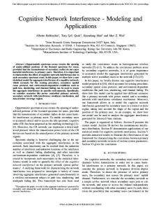
a function of the beacon detection threshold and the cognitive user density and transmit power. Subject to random fading and random cognitive user locations, this interference is random. We provide closed-form upper bounds on the mean and variance of this interference power. Taking into account the distance between the primary transmitter and receiver, together with the primary transmit power, we then link the mean and variance of the interference to the outage probability on the primary user, therefore quantifying the effect of these cognitive users. The paper is organized as follows. In Section II, we introduce the detailed network model, the channel model and analyze the signaling system with beacon. We the formulate the interference from the cognitive users to the primary user in Section III. In Section IV, we derived closed-form upper bounds on the mean and variance of this interference. Section V links these mean and variance to the primary outage probability. We conclude in Section VI. II. N ETWORK AND SYSTEM MODELS A. Network model We consider a planar network with a single primary user and n cognitive users. The primary user is at the center of the network with the transmitter Tx0 and the receiver Rx0 at a distance R0 away. Surrounding the primary user are n cognitive users, each has a single transmitter communicating with a single and unique receiver. In examining the interference from these cognitive users to the primary user, we choose to center the network at the primary receiver Rx0 . The cognitive transmitters Txi and receivers Rxi (i = 1 . . . n) are then uniformly distributed in a circle centered at Rx0 of radius R. The average cognitive user density is constant at λ users per unit area. Thus the network area, in particular the radius R, grows with n. To limit the interference from each cognitive transmitter, we also assume that the cognitive transmitters must be at least a distance ² from the primary receiver, for some ² > 0. This practical constraint basically disallows the interfering transmitter to be at the same point as the interfered receiver. Implicitly, we assume that the cognitive users can detect the location of the primary receiver using some sensing mechanism, therefore they can abide by this rule. Figure 1 illustrates this network model. B. Channel model We study a wireless channel with path loss and fading. Given a distance d between the transmitter and the receiver, the composite channel h can be written as A ˜ (1) h = α/2 h d where A is a frequency-dependent constant, α is the power path ˜ is the small-scale fading factor. Assuming no line-ofloss, and h ˜ sight, h is a complex circular Gaussian random variable with zero
When a cognitive user misses the beacon, that user can transmit concurrently with the primary user with a probability that is its activity factor. Here we assume that all cognitive users have the same activity factor β and transmit with the same power P . Let xi the the transmit signal of cognitive user i, and x0 be the primary transmit signal, then the received signal at the primary receiver can be written as n X y0 = h 0 x 0 + Fi h i x i + z 0 (6)
0
Tx
0
R
Rx
i
Tx
i
Rx
ε
R0 θ
i=1
r
Fig. 1. Network model: The primary receiver is located at the center of the circle, the primary transmitter at a distance R0 , and the cognitive users are uniformly distributed in between the circles of radii R and ². Also shown is an example of a cognitive transmitter at radius r and angle θ.
where • Fi is an indicator function for cognitive user i transmitting; in other words, Fi is a random variable with the following density: ½ 1 with probability βqi (7) Fi = 0 with probability 1 − βqi
and the Fi are independent. z0 ∼ N (0, σ 2 ) is the additive white Gaussian noise. We assume that the cognitive users do not cooperate, hence xi are independent, zero-mean signals with power P . The total interference power from the cognitive users therefore is •
mean and unit variance. For simple notation, we assume A = 1 (which is equivalent to normalizing the noise power according to A). We denote the channel from primary Tx0 to primary Rx0 as h0 , from primary Tx0 to cognitive Rxi as gi , and from cognitive Txi to primary Rx0 as hi . Hereafter, we use the same channel notation with a tilde to denote the small-scale fading component in each channel. C. Signal model Each cognitive user has an active factor of β, which is the probability that the user is actively transmitting. To avoid interference to the primary receiver, the cognitive users listen to a beacon, which the primary transmitter sends before its own transmission. Upon receiving this beacon, the cognitive users will remain silent for the duration of the primary transmission. Denote xb as the beacon transmit signal and yi,b as the received signal at Rxi (for i = 1, . . . , n). Then yi,b can be written as yi,b = gi xb + zi .
i = 1, . . . , n
(2)
where zi is independent additive white Gaussian noise with power σ 2 . With the beacon transmit power Pb , then the received power at the cognitive receiver i is Pb |gi |2 . (3) σ2 We assume that a cognitive user can correctly decode the beacon if its receive power is above a threshold Pth . Therefore the probability that the cognitive receiver misses the beacon is · ¸ ¤ £ i Pth σ 2 2 qi = Pr Pr,b < Pth = Pr |gi | < . Pb i = Pr,b
Now denote
γ= then
Pth σ 2 , Pb
£ ¤ qi = Pr |gi |2 < γ .
(4) (5)
Note that γ is unitless since the noise power has been normalized by the path loss constant A.
I0 =
n X
Fi |hi |2 P.
(8)
i=1
Because of the random cognitive user location and the smallscaled channel fading, this interference power is a random variable. With a large number of independent cognitive users, the interference will appear as Gaussian. Thus the capacity-optimal primary transmit signal x0 is zero-mean Gaussian. With transmit power P0 , the rate achieved by the primary user is ¶ µ |h0 |2 P0 . (9) C0 = log 1 + I0 + σ 2
Since the interference power I0 is random, this capacity is also random. An outage probability for a given rate threshold T can then be defined as pe = Pr[C0 ≤ T ]. (10) Next we examine the interference power I0 and its effect on the primary outage probability. In particular, we will study the mean and variance of I0 in the limit as the number of cognitive users n → ∞. III. I NTERFERENCE FROM THE COGNITIVE USERS In this section, we compute the interference from all cognitive transmitters to the primary receiver. From our network model, the primary receiver is located at the center of the network, with the primary transmitter at a distance R0 away. The cognitive transmitters are uniformly distributed with constant density λ between two circles of radii ² and R. As the number of cognitive users grows, R approaches ∞. We will first establish the interference to the receiver from a cognitive transmitter at a radius r (² ≤ r ≤ R) and at an angle θ to the line connecting the primary transmitter and receiver, as in Figure 1. For uniformly distributed cognitive users, r has the density 2r , ² ≤ r ≤ R. (11) fr (r) = 2 R − ²2
The distribution of θ is uniform between 0 and 2π. Now consider the probability that this cognitive user misses the beacon, qi . From (1), the channel between the primary transmitter and this cognitive user is gi =
g˜i d(r, θ)α/2
(12)
where d(r, θ) = (r 2 + R02 − 2rR0 cos θ)1/2 .
(13)
Given this cognitive user location, then the probability of missing the beacon (5) becomes £ ¤ £ 2 ¤ qi = Pr |gi |2 < γ = Pr |˜ gi | < γdα (r, θ) . (14)
With g˜i being zero-mean circularly complex Gaussian, 2|˜ gi |2 is a chi-square random with 2 degrees of freedom with the £ variable ¤ pdf e−z , hence Pr |˜ gi |2 ≤ y0 = 1 − e−y0 . The missing beacon probability thus can be explicitly calculated as qi = 1 − e
α
−γd (r,θ)
.
(15)
When missing the beacon, the cognitive transmitter may transmit with probability β. The channel from this cognitive transmitter to the primary receiver is ˜ i |2 . hi = r−α |h
(16)
Since the cognitive transmitters are independent, from (8), (15), and (16), the total interference power from cognitive users can be written as n X ˜ i |2 I0 = P β (17) qi r α |h i
i=1
where
n qi d(ri , θi ) ri θi ˜ hi
= λπ(R2 − ²2 ) α = 1 − e−γd (ri ,θi ) (ri2 + R02 − 2ri R0 cos θi )1/2 2r , ² ≤ ri ≤ R , ∼ fri (r) = 2 R − ²2 ∼ U[0, 2π] i.i.d. ∼ N (0, 1) i.i.d.
i.i.d.
and α, β, γ, λ, R are constants. Denote =
˜ i |2 qi riα |h
(18)
then Ii are i.i.d. and I0 = P β
n X
Ii .
(19)
i=1
A. An upper bound on the interference Here, we apply some simple bounds to the interference that allow closed-form expressions. For simplicity, we will drop the subscript i of each cognitive user and denote d
=
I
=
Next, we will use this bound to study the mean and variance of the interference. IV. M EAN AND VARIANCE OF THE INTERFERENCE POWER
In this section, we study the mean and variance of the interference power. In particular, we will provide closed-form upper bounds on them. Since the interference power is a sum of i.i.d. random variables (19), and noting that n = λπ(R2 − ²2 ), the mean and variance of the interference power can be written as E[I0 ] = P βλπ(R2 − ²2 )E[I] ¡ ¢ var(I0 ) = P 2 β 2 λπ(R2 − ²2 ) E[I 2 ] − E[I]2
(21) (22)
Therefore, it is of interest to compute E[I] and E[I 2 ]. ˜ is a zero-mean circular complex Gaussian random Since h ˜ 2 ] = 1 and E[|h| ˜ 4 ] = 3. Noting the variable, we have E[|h| density of r in (11) and that θ is uniform, based on (20), we can bound E[I] and E[I 2 ] as Z R³ ´ r1−α α dr (23) 1 − e−γ(r+R0 ) E[I] ≤ 2 R 2 − ²2 ² Z R³ ´ 1−2α α 2 r dr (24) E[I 2 ] ≤ 6 1 − e−γ(r+R0 ) 2 R − ²2 ²
Next, we will evaluate these bounds on the mean and variance of the interference power. A. Upper bound on the mean interference power
=
Ii
distance, as if the cognitive user is located on the circle centered at the primary transmitter with radius r + R0 . The cognitive user then will be more likely to miss the beacon and therefore increase its interference to the primary user. This the interference can then be bounded as ³ ´ α ˜2 I ≤ 1 − e−γ(r+R0 ) r−α |h| (20)
(r 2 + R02 − 2rR0 cos θ)1/2 ´ ³ α ˜ 2. 1 − e−γd r−α |h|
We can bound the beacon missing probability by changing the distance from the cognitive user to the primary transmitter for the beacon reception. An upper bound corresponds to increasing this
Consider the upper bound in (23). Noting that 1 − α < 0, we have r 1−α ≥ (r + R0 )1−α ; hence ¢ α Z R ¡ 1−α 2 r − e−γ(r+R0 ) (r + R0 )1−α E[I] ≤ dr. R 2 − ²2 ²
To interpret this bound, note that the interference from a cognitive user can be seen as the interference when that user always transmits minus the portion during the time this user receives the beacon. The above bound corresponds to slightly reducing the latter portion by increasing the distance to the primary Tx from the cognitive user when that user receives the beacon. Hence the interference from this user when missing the beacon will be slightly increased. This bound can be evaluated in closed forms using the incomplete Gamma function, as shown in the Appendix. Specifically, we have an explicit upper bound for the average interference power E[I0 ] in (25). With an infinite number of cognitive users, R → ∞, this bound approaches a limit as in (26). Figure 2 shows a plot of this upper bound on E[I0 ] versus the beacon threshold level γ for α = 2.1, R0 = 5, ² = 0.2 (assuming a large R , R = 100000, and all other parameters normalized to unit values). We see that as the beacon threshold increases, the cognitive users are more likely to miss the beacon and therefore increase the average interference to the primary user. The case when the cognitive transmitters are always transmitting (a beaconless system) corresponds to γ = ∞. This limit, however, is
2πλβP α−2
≤
E[I0 ]
·µ
1
1
−γ(²+R0 )α
2−α
(² + R0 ) +e − α−2 − e ²α−2 R ¶ µ ¶¶¸ µ µ 2 2 α α (α−2)/α , γ(² + R0 ) , γ(R + R0 ) −Γ +γ Γ α α
≤
E[I0 ]
·
2πλβP α−2
1 ²α−2
−e
−γ(²+R0 )α
(² + R0 )
2−α
+γ
Γ
¶ (25)
µ
2 , γ(² + R0 )α α
¶¸
(26)
100
73.5 0
Upper bound on E[I ]
(α−2)/α
(R + R0 )
2−α
reduce to zero.
74
90
0
Upper bound on E[I ]
73
72.5
72
71.5 −2 10
−1
0
1
10 10 Beacon detection threshold γ
10
74 72 70 68 66 64 62 60 −2 10
−1
10
0
1
10 10 Primary Tx−Rx distance R0
2
10
Fig. 3. The upper bound on the average interference versus the primary Tx-Rx distance.
Similarly, Figure 4 shows the plots of the bound versus the receiver guard radius ². As ² increases the interference power monotonically decreases to zero, since the number of interfering transmitters around the primary receiver will asymptotically
70 60 50
30 −2 10
Fig. 4.
approached quickly for finite values of γ. The convergence rate depends on other parameters such as α, R0 , ² and P . Figure 3 shows the plots of this bound versus the primary Tx-Rx distance R0 (for α = 2.1 and γ = 0.2). The bound is monotonously increasing in R0 . As R0 increases, however, the interference upper bound approaches a fixed limit. Since most of the interference comes from the cognitive transmitter close to the primary receiver, when this receiver is far away from the primary transmitter (R0 is large), then these cognitive users are likely to always miss the beacon and hence create a constant interference level to the primary user.
80
40
Fig. 2. An upper bound on the average interference versus the beacon threshold level.
Upper bound on E[I0]
−γ(R+R0 )α
−1
10
0
10 Receiver guard radius ε
1
10
2
10
The upper bound on the average interference versus the guard radius ².
B. Upper bound on the variance of interference Similarly, noting that (r + R0 )α ≥ rα + R0α , the upper bound on E[I 2 ] in (24) can be further bounded as in (27), where the function F is given in the Appendix. Using the gamma functions as shown in the Appendix, this bound can be evaluated in closedform. From (22), (23) and (24), we deduce that as R → ∞, var(I0 ) depends only on E[I 2 ] but not E[I]. Thus when R → ∞, we have an upper bound on the variance of the interference to the primary user as in (28), where the function G is defined in (29). Figure 5 shows a plot of this upper bound on var[I0 ] versus the beacon threshold level γ for α = 2.1, R0 = 5, ² = 0.2, and all other parameters normalized to unit values. Compared to Figure 2, the beacon threshold has the opposite effect on the variance as it has on the mean: the variance is decreased at larger threshold levels. Thus increasing the beacon threshold also increase the interference but make it less variable. Conversely, by making the cognitive receiver more sensitive to the beacon, the interference is reduced on the average but is more variable. Figure 6 shows the plots of this bound versus R0 (for α = 2.1 and γ = 0.2). As a function of R0 , the variance has a unique maximum value, achieved at a “critical” (though small) R0 . When R0 is above a certain threshold, the variance stays constant. Similarly, Figure 6 shows the plots of this bound versus ². The bound is monotonously decreasing in ², and it approaches 0 quickly as ² increases. This implies that as ² increases, the interference from the cognitive users approaches a constant. V. O UTAGE PROBABILITY In this section, we relate the probability of outage on the primary user to the cognitive users’ activities, in particular, to the
E[I 2 ]
≤ =
Z R³ ´ 6 1−2α −2γR0α −2γr α 1−2α 1−2α −γ(r+R0 )α dr r e (r + R ) + e r − 2e 0 R 2 − ²2 ² ¸ · −2(α−1) 6 ² − R−2(α−1) −2γR0α F (α, 1 − 2α, 2γ, ², R) . − 2F (α, 1 − 2α, γ, ² + R , R + R ) + e 0 0 R 2 − ²2 2(α − 1) var(I0 )
6P 2 β 2 λπ
≤
µ
(28)
¶ 2 α , γx . α
(29)
α 1 1 1 − G(α, γ, ² + R0 ) + e−2γR0 G(α, 2γ, ²) 2(α − 1) ²2(α−1) 2
α α 1 αγ αγ 2−2/α G(α, γ, x) = e−γx x−2(α−1) − e−γx x2−α + Γ (α − 1) (α − 1)(α − 2) (α − 1)(α − 2)
µ
(27)
1400
460 440
1200
Upper bound on E[I ]
0
0
Upper bound on var[I ]
420 400 380 360 340
1000 800 600 400
320 200
300 280 −2 10
−1
10
0
1
10 10 Beacon detection threshold γ
0 −1 10
2
10
Fig. 5. An upper bound on the variance of the interference versus the beacon threshold level. 550
450 0
Upper bound on E[I ]
1
2
10
Fig. 7. The upper bound on the variance of the interference versus the receiver guard radius ².
and denote the noise-to-signal ratio (the inverse of SNR) per bit at the target rate as σ2 ξ= , (31) Pr
500
400 350
then the outage probability becomes ³ ´i h ˜ 0 |2 − ξ . pe = Pr I0 > Pr |h
300 250 200
(32)
The outage can be separated into two parts: outage due to noise alone, pn , and outage due to interference, pi
150 100 50 −2 10
0
10 10 Receiver guard radius ε
−1
10
0
1
10 10 Primary Tx−Rx distance R
pe = p n + p i
2
10
0
Fig. 6. The upper bound on the variance of the interference versus the primary Tx-Rx distance.
mean and variance of the interference power I0 . With the primary user rate (9), given a target rate T , the outage probability can be written as # " ˜ 0 |2 P | h 0 . pe = Pr [C0 < T ] = Pr I0 + σ 2 > R0α (2T − 1)R0α Denote the following expression as the “normalized” (without the channel) primary received power per bit at the target rate: P0 Pr = T (2 − 1) R0α
(30)
(33)
where h i ˜ 0 |2 ≤ ξ = 1 − e−ξ pn = Pr |h ³ ´ i h ˜ 0 |2 − ξ , | h ˜ 0 |2 > ξ pi = Pr I0 > Pr |h ³ ´¯ i h ˜ 0 |2 − ξ ¯¯ |h ˜ 0 |2 > ξ . = e−ξ Pr I0 > Pr |h
(34)
(35)
Lets investigate the outage due to interference, pi . Denote ³ ´ ˜ 0 |2 − ξ = P r |h ˜ 0 |2 − σ 2 , t = P r |h (36)
then
pi = e−ξ Pr [ I0 > t| t > 0] .
(37)
In this expression, both I0 and t are random variables. From (19), since the interferences from different cognitive users are independent, based on the LLN, as n → ∞, I0 approaches a
Gaussian random variable with mean E[I0 ] and variance var(I0 ). ˜ 0 |2 is an exponential random variable On the other hand, since |h with parameter 21 , the pdf of t is given as µ ¶ 1 t + σ2 ft (t) = exp − , t ≥ −σ 2 . 2Pr 2Pr
We will now bound the probability Pr[I0 > t] for a given t, then compute pi in (37) using the distribution of t. For a given t, using the Chernoff bound on a Gaussian random variable, we have ¶ µ (t − E[I0 ])2 Pr[I0 > t] ≤ exp − 2var(I0 ) Now taking in the distribution of t, the conditional probability in pi can be upper bounded as in (38).
Pr[I0 > t|t > 0] ¶ µ ¶ µ Z ∞ 1 t + σ2 (t − E[I0 ])2 exp − dt ≤ exp − 2var(I0 ) 2Pr 2Pr 0 ¶ µ σ2 E[I0 ] var(I0 ) 1 exp − − + = 2Pr 2Pr 2Pr 8Pr2 ¶ µ Z ∞ 2 x × dx. (38) exp − var(I ) 2var(I0 ) −E[I0 ]+ 2P 0 r
We can further bound this probability as follows. Noting that the lower limit of the integral in (38) depends on the received power Pr and the mean and variance of the interference I0 , we consider two cases. When the received power Pr (30) is large enough such that var(I0 ) , (39) Pr ≥ 2E[I0 ] then the lower integral limit is non-positive. Using the whole Gaussian density integral, we can upper bound (38) as Pr[I0 > t|t > 0]] p µ ¶ 2πvar(I0 ) σ2 E[I0 ] var(I0 ) exp − − + ≤ . 2Pr 2Pr 2Pr 8Pr2
R EFERENCES [1] FCC, “FCC ET docket no. 03-108: Facilitating opportunities for flexible, efficient, and reliable spectrum use employing cognitive radio technologies,” Tech. Rep., FCC, Dec. 2003. [2] J.Mitola, Cognitive Radio, Ph.D. thesis, Royal Institute of Technology (KTH), 2000. [3] S.A. Srinivasa, S.; Jafar, “Cognitive radios for dynamic spectrum access the throughput potential of cognitive radio: A theoretical perspective,” IEEE Communications Magazine, vol. 45, no. 5, pp. 73–79, May 2007. [4] N. Devroye, P. Mitran, and V. Tarokh, “Achievable rates in cognitive radio channels,” IEEE Trans. on Information Theory, vol. 52, no. 5, pp. 1813–1827, May 2006. [5] K. Liu Q. Zhao, B. Krishnamachari, “Low-complexity approaches to spectrum opportunity tracking,” Crowncom Conf., Aug 2007.
A PPENDIX G AMMA FUNCTION EVALUATIONS We denote the following function which is used in the bounds on the mean and variance of the interference power: Z v α e−γz z β dz. F (α, β, γ, u, v) = u
(40)
In the case that (39) does not hold, denote w as the lower limit of the integral in (38), then w ≥ 0. For the integral range, since x ≥ w ≥ 0, replacing x2 by xw, we obtain another bound for (38) as Pr[I0 > t|t > 0] µ ¶ 2var(I0 ) σ2 E[I0 ]2 ≤ exp − − . var(I0 ) − 2Pr E[I0 ] 2Pr 2var(I0 )
and receiver, and the receiver protected radius. We then provide closed-form upper bounds on the mean and the variance of this interference power, both with a finite number of cognitive users and in the limit as this number goes to infinity. These bounds offer an analytical understanding of how the interference behaves according to various network parameters. We also relate the mean and variance of the cognitive interference power to the outage probability of the primary user. These analytical results can help a network designer in setting the network parameters to meet a required performance goal. The beacon model in this paper can also be generalized to a broader side information model in cognitive networks. Interference analysis in such networks will be important in understanding the interaction among the users and in designing their algorithms.
(41)
Then combining (33) with (34), (37) and (40) or (41), we obtain an explicit bound on the outage probability that is a function of the mean and variance of the interference power I0 and other parameters. VI. C ONCLUSION In this paper, we studied a network consisting of a primary user and multiple cognitive users. The primary user sends a beacon prior to each transmission to silence the cognitive users and claim the spectrum. But because of channel fading, there is a nonzero chance that a cognitive user misses this beacon and transmits concurrently with the primary user, hence creating interference. We formulate this interference power as a function of the beacon threshold, the number of cognitive users. the primary and cognitive transmit powers, the distance between the primary transmitter
To evaluate this function, let w = z α , dw = αz α−1 dw = αw(α−1)/α dz, then
= = =
F (α, β, γ, u, v) Z vα dw e−γw wβ/α (α−1)/α αw α u Z γvα dx e−x (x/γ)β/α , (α−1)/α αγ(x/γ) α γu Z α γ −(β+1)/α γv −x (β+1)/α−1 e x dx. α γuα
(x = γw)
If β + 1 ≥ 0, then
F (α, β, γ, u, v) (42) ¶ µ ¶¸ · µ −(β+1)/α γ β+1 β+1 = , γuα − Γ , γv α . Γ α α α
where Γ(·, ·) is the incomplete Gamma function. If β + 1 < 0, then F (α, β, γ, u, v) ´ α 1 ³ −γvα β+1 = e v − e−γu uβ+1 β+1 αγ + F (α, β + α, γ, u, v) . β+1
(43)