To achieve this goal, in a process we call location certification, data routed through ... Corresponding Author's address: R. Sion, Computer Science, Stony Brook ...
Collaborative Location Certification for Sensor Networks JIE GAO, RADU SION, SOL LEDERER Network Security and Applied Cryptography Lab Computer Science, Stony Brook University {jgao, sion, lederer}@cs.stonybrook.edu.
Location information is of essential importance in sensor networks deployed for generating location-specific event reports. When such networks operate in hostile environments, it becomes imperative to guarantee the correctness of event location claims. In this paper we address the problem of assessing location claims of un-trusted (potentially compromised) nodes. The mechanisms introduced here prevent a compromised node from generating illicit event reports for locations other than its own. This is important because by compromising “easy target” sensors (say, sensors on the perimeter of the field that’s easier to access), the adversary should not be able to impact data flows associated with other (“premium target”) regions of the network. To achieve this goal, in a process we call location certification, data routed through the network is “tagged” by participating nodes with “belief” ratings, collaboratively assessing the probability that the claimed source location is indeed correct. The effectiveness of our solution relies on the joint knowledge of participating nodes to assess the truthfulness of claimed locations. By collaboratively generating and propagating a set of “belief” ratings with transmitted data and event reports, the network allows authorized parties (e.g. final data sinks) to evaluate a metric of trust for the claimed location of such reports. Belief ratings are derived from a data model of observed past routing activity. The solution is shown to feature a strong ability to detect false location claims and compromised nodes. For example, incorrect claims as small as 2 hops (from the actual location) are detected with over 90% accuracy. Finally, these new location certification mechanisms can be deployed in tandem with traditional secure localization, yet does not require it, and, in a sense, can serve to minimize the need thereof. Categories and Subject Descriptors: C.2.2 [Computer Systems Organization]: COMPUTERCOMMUNICATION NETWORKS General Terms: Algorithms, Systems Additional Key Words and Phrases: Sensor Networks, Security, Location Certification
1. INTRODUCTION Node location information plays a fundamental role in ad-hoc networks. Specifically, in sensor networks, it is critical that the reported location of all nodes are Corresponding Author’s address: R. Sion, Computer Science, Stony Brook University, Stony Brook, NY 11794. In part supported by the NSF (IIS-0803197, CNS-0627554,0716608,0708025), IBM, Xerox and CEWIT. Permission to make digital/hard copy of all or part of this material without fee for personal or classroom use provided that the copies are not made or distributed for profit or commercial advantage, the ACM copyright/server notice, the title of the publication, and its date appear, and notice is given that copying is by permission of the ACM, Inc. To copy otherwise, to republish, to post on servers, or to redistribute to lists requires prior specific permission and/or a fee. c 20YY ACM 0000-0000/20YY/0000-0001 $5.00 ° ACM Journal Name, Vol. V, No. N, Month 20YY, Pages 1–0??.
2
·
Gao, Sion, Lederer
accurate, to ensure a point of reference for location-specific applications. Thus, a robust network must require such information be un-compromised, lest a few faulty or malicious nodes will have a deleterious effect on the entire network. Existing work investigates secure localization [Lazos and Poovendran 2004], i.e., how nodes determine their own location in a hostile environment, and secure location verification [Sastry et al. 2003; Waters and Felten 2003], determining the location of a node in the face of liars. Typically these protocols involve special anchor nodes, or nodes whose location is not corruptible. Based on the distance to these nodes, the location of the remaining nodes is determined with certain assurances by deploying distance-measuring RF or ultrasound-based mechanisms and performing multi-way handshakes under synchronized clocks assumptions. These methods are designed to be used when the network is first deployed, to establish the location of all nodes during its initial setup. However, when operating in hostile environments, it is essential to secure location information claims at runtime, in the presence of compromised nodes, that could falsify location claims and inject incorrect event reports into the information stream. False location information may lead the data sink to take action in a location where none is warranted, and vice versa, not take action in the area where a response is necessary. We introduce a protocol that validates the truthfulness of location information associated with event reports. The protocol relies on the collaborative interaction of the network nodes to find compromised parties. Since each node is an active participant in the network and spends a substantial amount of time and resources relaying messages for others, it automatically has some knowledge of the activity within the network. This knowledge can be put to good use in spotting anomalous behavior. The workload and detection ability is thus distributed across the network, to avoid a single point of failure and gracefully degrade with increasing number of compromised nodes. To achieve this purpose, at an overview level, nodes in the network (compactly) record summaries of routing paths taken by packets through the network. Upon receiving a packet, nodes examine whether their route matches a historically expected behavior by packets from the same claimed location. A belief about the correctness of this location claim of this packet is then created and propagated to the data sink, either as part of this packet or later on, in an out of band fashion. The attached beliefs will be used by the authorized packet evaluators PEs (sinks or authorized intermediate relay nodes) to certify the truthfulness of the packets’ location information. We show by simulations that the belief rating has a strong correlation with the deviation of the source’s real location from its claimed location. Thus if a node lies about its location, the farther away it claims to be from its real location, the more likely the packets will be identified. The memory limitations of sensor nodes require light-weight protocols both in terms of memory and power usage. Accordingly, we developed a path metric and a compact way to express path trajectories, by using locality-sensitive hashing [Indyk and Motwani 1998]. This metric captures the fact that packets from sources with incorrectly claimed locations are likely to have path trajectories deviating from ACM Journal Name, Vol. V, No. N, Month 20YY.
Collaborative Location Certification for Sensor Networks
·
3
previously observed traffic paths. The key advantage of our solution lies in its collaborative nature and in the involvement of the network in a community of trust. A single malicious or faulty node is unlikely to take over the entire network and cause significant damage. To better understand the challenge of the problem and the rationale of our approach, we also outline the following alternative straight-forward schemes. —Immediate neighbor detection. An immediate neighbor (p) of the malicious node could detect that it is not in the region it claims, because this region is out of the communication range of p. This scheme is vulnerable to multiple (two) adversarial colluding nodes; the adversary directly communicating with p would not actually be lying about its location. Moreover, in general the problem is more significant, because an adversary can “create” a whole set of fake nodes b1 , b2 , · · · , bk where the distance between any bi and bj is within the communication radius R, and the distance between bk and the true node is more than R. Even by looking at the distances between all the nodes on the path and ensuring that the distance between any two consecutive nodes is short, an honest node cannot determine if there is a node lying about its location. —Distance from straight line trajectory. A simple idea for a scenario where the sensor nodes are densely and evenly distributed throughout the region is to compute how far the current node lies off the straight line trajectory between the source node and the sink. Based on how far away from the direct path this node lies should the belief rating be made. However, this mechanism would fail in the case of irregularities in the network. Specifically, when there are holes in the network, or when routing paths do not follow straight line paths, a node may well be placed far from the straight line from source to destination — also observed in real experiments [Zhou et al. 2004]. As shown later, our path metric is adaptive to these variations in traffic patterns. We capture the case when a packet follows a path not “similar” to the expected ones, in which case the packet will be tagged with a poor belief rating. Secure Localization vs. Location Certification Finally, it is important to outline the difference between secure location certification and traditional secure localization, because, apparently, by using secure localization in an initial stage, nodes could propagate location information securely to the data sink and then simply authenticate each future even reports. The sink will associate these reports with the known previously received location information of each node. The above apparent localization-based solution in fact illustrates a great example on why location certification is needed. Indeed, if we assume secure localization happened, now if a node is compromised (including its shared key with the sink), the adversary (e.g., battle-field enemy) can simply move the sensor to a less dangerous (for the adversary – e.g., less monitored) location and now inject false event reports about the node’s assumed (original) location into the network. Location certification can prevent this. Moreover, often secure localization is not an option due to both communication costs and hardware/beacon requirements and as such is not a prerequisite of our mechanisms which, in a sense can serve as a poor man’s replacement thereof. Naturally, certain nodes will be required to have the ability to locate themselves ACM Journal Name, Vol. V, No. N, Month 20YY.
4
·
Gao, Sion, Lederer
securely in one way or another, yet overall, most of the network nodes are not assumed to be aware of their location. Similarly, the sink is NOT assumed or required to know individual locations. We believe this is essential in order to allow the deployment of ad-hoc networks composed of extremely cheap hardware with minimal localization ability for individual nodes. Moreover, many of the nodes in the network could be sporadic and/or routing-only and not participate in the protocol. Location certification can involve all nodes in collaboratively assessing location claims without necessarily having the ability to do localization. The paper is structured as follows. We introduce the sensor model and the adversary model in section 2. In section 3 we discuss collaborative location certification, and the belief rating generation and propagation. Both the metric and the detection ability are evaluated by simulations in section 7. In section 8 we overview related work on location certification and secure localization algorithms. 2. MODEL In this section we discuss the considered adversarial and deployment models. 2.1 Adversary Of concern here is a malicious, powerful adversary with strong incentives to capture and compromise sensors for the purpose of altering the sensor data flow, e.g., by inserting false data and event reports and eventually influencing decision making process at the base station. For such an adversary, pure denial of service (DOS) attacks that aim to disable sensors and parts of the network are only of marginal interest and will not be considered here. For DOS attacks, [Wood and Stankovic 2002; Cheung et al. 2005] offer techniques to address these issues. Multi-path forwarding [Karlof and Wagner 2003] alleviates the problem of malicious relay nodes dropping legitimate reports. Also, by using a cache to store the signatures of recently forwarded reports we can prevent against the same packet from being replayed [Ye et al. 2003; Intanagonwiwat et al. 2000]. Finally, by encrypting the event reports and any associated data with keys shared with data sinks, confidentiality and data integrity can be achieved. In particular, the mechanisms introduced here provide correctness assurances of node location claims in the process of event reporting. They prevent a compromised node from generating illicit event reports for locations other than its own. This is important because by compromising “easy target” sensors (say, sensors on the perimeter of the field that’s easier to access), the adversary should not be able to impact data flows associated with other (“premium target”) regions of the network. To achieve this goal, data routed through the network will be “tagged” by participating nodes with “belief” ratings, collaboratively assessing the probability that the claimed source location is indeed correct. We call this process location certification. To circumvent location certification (e.g., for the purpose of injecting fake event reports referencing remote, out of reach locations) an adversary could attempt to: (i) favorably modify certificates for its own fake data (e.g., by altering the associated belief ratings), or (ii) unfavorably alter certificates of legitimate traffic. The probability of success of such attempts is naturally related to the density of ACM Journal Name, Vol. V, No. N, Month 20YY.
Collaborative Location Certification for Sensor Networks
·
5
compromised nodes in the network. The ability of success adapts gracefully to the density of compromised nodes and the solution can operate even in the presence of a large number of adversarial nodes, as validated through simulations. For illustration purposes, we first consider an adversary that only attempts to maliciously claim a different location in its event reports (but does not maliciously alter belief ratings of other packets it routes). We then discuss additional security issues in section 4. 2.2 Deployment. Routing. We focus in this paper primarily on monitoring networks in which the sensors collect information of interest and send data/event reports to a base station (data sink) for post-processing and analysis. To this end we assume the existence of a training period (e.g., immediately after deployment) in which the network is assumed free from any adversarial presence. Since our location certification procedure is based on using past history of network routes, we must assume that the original history is initially “clean”. The better the history data is in terms of “cleanliness”, the better the location certification will perform. Since history data is used to predict future network behavior, we assume that the network is to some degree consistent in its routing behavior. If strong routing patterns are exhibited, i.e., all packets from the same source are typically routed along similar paths, then location certification will perform well. If the legitimate routing behavior is completely random (say packets from the same source take arbitrary routing paths) then our protocol won’t work well. Naturally, geometric routing maintains a high degree of consistency in routing patterns, so we generally will speak in terms of a geometric routing protocol, and this is the routing scheme used in our simulations. However, geometric routing is not a prerequisite for the protocol. Finally, we note that in the most general case (i.e., in the absence of trusted GPS beacons and location information for all nodes – we do not require secure localization) our mechanisms’ accuracy/resolution is a direct function of network node density. Specifically, in a network composed of very few nodes communicating over long distances, a node maliciously claiming the location of a direct (network) neighbor (possibly hundreds of feet away) and then routing the packet correctly will not be detected by our or any existing mechanisms. In our case this is because the detection resolution is directly related to the number of nodes on the route path for the suspicious event report (and thus on average to the network density). 3. COLLABORATIVE LOCATION CERTIFICATION In this section we detail the main components of the location certification protocol. 3.1 Solution Overview At an overview level, the proposed solution unfolds as follows. Independent of our mechanisms, traditional network secure localization protocols [Lazos and Poovendran 2004] will allow a subset of the sensors to acquire location information that is to be later used in event reports. Existing research achieves this by assuming a largely un-compromised network for a short amount of time after deployment. We ACM Journal Name, Vol. V, No. N, Month 20YY.
6
·
Gao, Sion, Lederer
note that the existence of localization is not a pre-requisite of our protocol, which can co-exist and operate in parallel with it. Once the network becomes fully operational, sensors will start generating event reports associated with their respective location. A compromised sensor could then attempt to generate illicit event reports for locations other than its own. To defeat such an adversary, nodes along the path from the source to destination will attach “belief” ratings to passing data packets, quantifying the correctness probability of the claimed source locations. Informally, beliefs are a function of observed past traffic patterns in conjunction with the claimed source location. Upon receiving packets with routing information deviating from expected traffic patterns, nodes will have the opportunity to propagate negative belief ratings associated with these packets. The negative beliefs reflect the appearance of an anomaly in the routing pattern. Thus this scheme is able to detect both the case in which the routing pattern is altered by an adversary (a compromised node lies about its location, or other routing attacks such as wormhole attacks [Papadimitratos and Haas 2002; Hu et al. 2003; Sanzgiri et al. 2002]) and the case of node failures — a large fraction of nodes run out of battery power or get physically destroyed by adversaries causing significant routing pattern changes. A node which rarely participated in the data collection operation will get a low confidence, which is reasonable as the network collectively has little or no information to decide whether it is a legitimate node. We re-iterate that this solution assumes the network is initially free from adversaries for a short period of time. If a large number of compromised nodes is present at the start and they are able to generate arbitrary traffic patterns then collaborative certification will be less effective. In a typical deployment there is often a short period of time which is more than enough for our scheme to collect enough history traffic data. With this limitation in mind, we believe that the novelty in our scheme lies in the compact and efficient way of summarizing the history traffic pattern and the ability of using the history to verify the correctness of future packets. 3.2 Strawman’s Book-keeping. Before proceeding, to illustrate, we first discuss an extremely simple book-keeping mechanism, the understanding of which will motivate our final solution. As part of the routing protocol, each sensor will maintain a history and normalized count of each previously seen source-destination pair for routed packets. New incoming packets from rarely seen sources will then be considered more suspicious and associated with a low rating. While this scheme is extremely simple and scalable, it presents certain limitations, in particular in its ability to detect deviations in full routes (as opposed to endpoints). If a node does route information between the claimed origin and destination, then the packet from an adversary claiming to be from a different location will be considered fair game. To achieve a better detection accuracy, more information about information flow is required in the belief rating construction. 3.3 Inter-Path Distance Metric Accordingly, we explore first how to compare packet routes efficiently in a meaningful way. Based on the sequence of nodes a packet has visited, we derive a trajectory ACM Journal Name, Vol. V, No. N, Month 20YY.
Collaborative Location Certification for Sensor Networks
·
7
of a packet by the piece-wise linear curve connecting the intermediate nodes in their visited order. We define a distance metric that measures how far two trajectories are. The distance is designed such that fake claimed locations for packets will result in large distances between real and expected trajectories. There are many generic ways to measure the distance between two curves in space, such as Hausdorff distance and Frech´et distance. Here we design a measure well suited to our problem at hand. P
p1 p01
P0
pk
p0k
Fig. 1. The distance metric between two paths P, P 0 . In this figure we adopt a uniform parametrization and the samples are placed uniformly on the paths.
Given a trajectory P (a curve in the plane), we adopt a parametrization (e.g., uniform, but other parameterizations may also be used, as will be shown later) and take k samples {p1 , p2 , · · · , pk }, on P. We define the distance between two Pk paths P, P 0 as π(P, P 0 ) = i=1 ||pi − p0i ||2 , the sum of squared distance between corresponding sample points. From a different viewpoint if a path P is considered a point in 2k dimensional Euclidean space p = (p1 , p2 , · · · , pk ) (each point pi is a point on 2D), the distance between two paths is the squared `2 norm of their corresponding representative 2k-dim points. In our scenario the number of samples naturally corresponds to the sensor nodes on a path. A path of k − 1 hops maps to a 2k-dimensional point. In the following we will see this observation become very useful in the design of a succinct data structure that summarizes the relative distances of a set of paths by a set of points on a 1-dimensional line. Essentially each node will keep a compact structure (to be explained in section 5) that summarizes the trajectories of the packets that go through it. Once a new packet arrives, the current trajectory is compared against past trajectories of packets from the same source or nearby. See Figure 2 for an example where an adversarial node s sends a message that goes through a node u, but claims it is at location s0 . The path taken by the packet, P, is different from the path it should have taken if it is indeed generated from a node at s0 (shown as the dashed path P 0 ). This is exactly the type of discrepancies captured by our path metric. We use a parametrization scheme that samples uniformly in each hop. If a path has m hops, then each hop is sampled uniformly k times to yield a total of m × k sample points. 3.4 Locality Sensitive Hashing Yet, the full path history is too large for the packet to carry and for sensor nodes to keep. Consequently, we adopt locality sensitive hashing [Indyk and Motwani 1998] a mechanism perfectly suited to compress such data and represent each path by a single value. The distance between two paths then becomes the distance between ACM Journal Name, Vol. V, No. N, Month 20YY.
8
·
Gao, Sion, Lederer
s
P
u
P0 s0 Fig. 2. The real path P taken by a packet from s is different from the path P 0 it should have taken if it were generated from the claimed location s0 .
their compressed values. In general, locality sensitive hashing takes points in high dimensional space and maps them to 1D such that the Euclidean distances between them are roughly preserved. Recall that each path can be considered as a point in 2k-dimensional space, which is then hashed to a point in 1D such that the distance between any two paths is correlated to the distance between their corresponding 1D points. Locality-sensitive hashing makes use of the properties of stable distributions. A stable distribution [Datar et al. 2004] is a distribution the random variable P where P p 1/p |v | ) X, where X1 . . . Xn v X has the same distribution as the variable ( i i i i i are i.i.d. variables from that distribution. It is known that Gaussian distribution is stable for `2 norm. This means that if we represent a path P in our network by a vector in 2k-dimensional space v = (p1 , p2 , · · · , pk ) and generate a random vector a (with each element chosen uniformly randomly from a Gaussian distribution σ(0, 1)), of the same dimension, then taking the dot product of the two vectors, a · v, results in a scalar distributed as ||v||2 X, where || · ||2 is the `2 norm, and X is a random variable with Gaussian distribution σ(0, 1). It follows that for two vectors (v1 , v2 ) the distance between their hash values |a·v1 −a·v2 | is distributed as ||v1 − v2 ||2 X where X is a random variable of a Gaussian distribution. Therefore, if we have a vector vi , which represents a path in our network, we can generate a scalar value from it (by taking the dot product with a) that still maintains the property that its distance from another scalar generated by another vector v2 is correlated to the original “distance” between v1 and v2 as we previously defined. A hash function that uses random variables of a stable distribution to map high-dimensional vectors to 1D points satisfies the above definition of locality sensitivity. In our case the routing paths have different lengths and thus map to vectors of different lengths. Thus we assume that the random vector a is one of potentially infinite length and is generated by a pseudo-random function known to all the nodes in the network. Upon receiving a packet with observed trajectory vector v, each sensor will use locality sensitive hashing to store only the hashed value h(v) = a · v together with the location where this packet was generated. For a new packet that claims to be from the same region, the hashed value of the new packet is compared with the hashed values in the past history. A belief rating directly proportional to the difference of these two values is then generated. When a packet is routed, the routing path is revealed gradually. The hash value of the path is then updated. Essentially a packet received by u only carries k (the number of hops of the path so far), the position of the last node v visited and the ACM Journal Name, Vol. V, No. N, Month 20YY.
Collaborative Location Certification for Sensor Networks
·
9
hash value computed by v. u will then update the packet with its own location and the new hash. The new hash value is computed as the sum of the old hash plus the value (vx , vy ) · (a2k , a2k+2 ), where (ux , uy ) is the location of v, and ai is the ith element of the random vector a. As the locality sensitive hash is essentially the dot product of the location vector with the random vector, the update to the old hash yields the correct hash value, while significantly reducing the communication overhead. In section 7.1 we show how the use of locality sensitive hashing in the design of belief ratings results in a strong correlation between the distance a node is from a claimed location and the resulting belief. 3.5 Belief Generation By the property of locality sensitive hashing, packets taking paths similar or identical to each other tend to cluster together on the real line, while packets coming from unknown regions or following a highly irregular path map to different points. To express a correctness belief about the claimed location of incoming packets, their associated hash values are thus compared with the expected value ranges of nodes originating from the same region. We explain in section 5 how the hash values of different packets are stored and compared, and how we group hash values based on the path’s origin. Note that when the network is first deployed nodes do not have any history about the network. We allow the beliefs to evolve gradually over the lifetime of the network by having the belief rating be comprised of 2 values: one is the actual belief rating, the second is the belief confidence. Intuitively, the rating captures how well a new packet matches previous history data, while the confidence measures how much history data a node has at its disposal. If the confidence is low than the belief value is less useful. Initially, in a new network, the confidence values will be low, and the beliefs ratings will be of limited value. But as nodes accumulate history, belief ratings will be given with higher confidence. Note that if a new node comes online in a network where nodes have had time to assess sufficient history data then it will be given a rating with high confidence, good or bad depending on how well it conforms to past traffic patterns. The interplay between belief values and confidence values is complex and actual thresholds of what is considered a “good” rating or “bad” rating would depend on the particular network and/or application. These can be adjusted depending on the circumstances. The data structure we use captures both components of the belief rating. See Section 5. 3.6 Aggregating Ratings and Defeating Belief Skewing Attacks We first note that malicious nodes can not arbitrarily skew belief ratings for colluders or other “good” nodes as the final report rating is an aggregate of all the (encrypted and secured) ratings of the mostly trusted nodes routing the packet. We have not elaborated on this aggregate because we believe this is a mostly application-specific issue. Indeed numerous formulas can be deployed, from simple linear combinations of all the individual nodes’ ratings (e.g., weighted averaging) to complex Markov Model based mechanisms that account for node identity and time, space locality to arrive at a trust probability. For example, in the linear case (we used this in the experiments), if a majority of ACM Journal Name, Vol. V, No. N, Month 20YY.
10
·
Gao, Sion, Lederer
network nodes have been compromised, the rating could be weakened and malicious en-route nodes will have increasing ability to impact the rating of each packet. Yet, the good news is that the mechanism degrades gracefully and (it is easy to show that) in a uniformly distributed network, the upper bound on the illicit impact in the rating of any one event report is a linear function of the density of malicious nodes. We also note that the dynamic nature of the collaborative belief training requires mechanisms of preventing malicious nodes from skewing belief ratings by repeatedly sending incorrectly labeled event reports. We will not detail this beyond our scope, as it can be naturally achieved during the mitigation phase, once an alarm has been raised and a compromised node has been detected due to its attached (low) rating. In that case, the data sink will mark the compromised node as such and appropriately handle its further reports. The data sink will also contact the network and blacklist the node. This is not absolutely necessary – and the main reason for doing so is to prevent others to route their messages through the compromised node. For efficiency, in an initial phase, only the sensors on the path to the compromised node can be notified. Note that the above defense will likely still allow an adversary to very slowly “move” compromised nodes by sending numerous reports that will all be rated just below the alarm-threshold (because the claimed location is close enough to the original location for the compromised node). To further defeat such behavior, report frequency can be factored in the generation and (more importantly) evaluation of beliefs: even if a negative rating is below the alarm-raising threshold, if many such packets suddenly appear – the threshold could be further decreased temporarily, possibly only for the secret credential (encryption key) corresponding to the suspected compromised node. Alternately if such adaptive sink-driven action is not possible (power and efficiency constraints) or desirable, another straightforward solution to this issue is to not alter the internal nodes’ certification information (in other words to not re-train) after a certain period in time, or associate different weights to knowledge acquired in different segments of time/space depending on their associated network vulnerability exposure levels. 4. SECURITY We now describe how we prevent one or more colluding adversaries from tampering with the belief ratings or hash values of packets passing through. We want to ensure that (i) individual belief values are not tampered with in transit, (ii) packets containing incriminating ratings cannot be distinguished from other traffic, (iii) new fake belief values are not added to bad-mouth a packet or improve its rating, and (iv) existing belief ratings are not removed from packets. 4.1 Semantic Security To ensure the above, we first require that each sensor be associated with a unique, public identifier and with a secret, unique symmetric encryption key, known only to a very small set of authorized, un-compromised parties such as the data sink or a few intermediary relays, called packet evaluators, PEs. This is a reasonable, practical assumption to be found in existing research [C . amtepe and Yener 2005]. ACM Journal Name, Vol. V, No. N, Month 20YY.
Collaborative Location Certification for Sensor Networks
·
11
This key can then be used for communication between the sensor and the PEs. Such communication however, we require to be deployed using any semantically secure encryption cipher [Goldreich 2001] (e.g., any cipher running in CTR mode). Semantic security is necessary to prevent an adversary of correlating encrypted fields in the current packet with fields of previously seen ones (e.g., if they represent the same value). Our solution does not depend on the deployed encryption mechanism. Symmetric key cryptography has been chosen over public key crypto, due to the computation-limited platform assumed. While details are out of scope here, we note that more powerful mechanisms can be devised using asymmetric key primitives. Such mechanisms would allow optimized, in-network location claim evaluation and packet filtering, effectively reducing overhead induced by compromised traffic. 4.2 Secure Belief Propagation Upon generating a belief b (composed of a rating and confidence, see section 3.5 and hash for the current packet), a sensor i will encrypt it using its shared symmetric key with the sink ki and append the result Eki (b) to the packet. Requirements (i) and (ii) above are naturally handled. To ensure (iii) and (iv) we propose to use a cryptographic digest1 chain constructs. Specifically, upon propagating a new belief b with the current packet, a sensor i will perform two operations. First it will encrypt the belief as above Eki (b). Second, it will update the packet’s digest chain value c as follows: cnew ← H(cold |H(b)), where H is a cryptographic digest, and ‘|’ denotes concatenation. At the PEs end, each packet’s digest chain can be reconstructed and verified upon decrypting all beliefs. To selectively remove a rating from the packet, a malicious adversary is faced with having to correctly reconstruct a new digest chain for the remaining beliefs. This, however, will require the decryption of those beliefs (using secrets not in the possession of the adversary). Thus (iii) and (iv) are handled. An adversary can still attach a bad belief rating, i.e., bad-mouth a packet. But this is essentially denial of service attack in which the relay adversary can simply drop the packet from the data stream. As message digests over small amounts of data are extremely fast, the induced overhead is minimal. To summarize, a node receiving a packet will append an encrypted belief rating, update the digest chain as mentioned above and deliver the packet to the next hop. The way that nodes attach belief ratings can be adaptive to the network scenario and desired detection ability. We now introduce two belief generation and propagation methods. Stochastic Propagation. An immediate and natural extension to the above propagation mechanism is the use of a stochastic behavior reducing communica1 We
use “cryptographic digest” to denote a cryptographic hash function, so as to avoid any confusion with the locality sensitive hash constructs. We note that the collision resistance of such a hash function is not paramount here, given that the adversary would have a hard time finding meaningful collisions within a few minutes (and for a large enough number of packets to become meaningful), before the packet is due at the sink. We assume the hash function outputs 6 bytes. ACM Journal Name, Vol. V, No. N, Month 20YY.
12
·
Gao, Sion, Lederer
tion requirements while gracefully degrading security assurance levels. Specifically, sensors express beliefs only with a certain probability ps ∈ (0, 1]. Upon receiving an incoming packet, a node will uniform randomly decide whether to generate and propagate its current belief. Naturally, ps will now determine the efficiency of the solution; lower values will result in less beliefs propagated but also lower communication overhead. Nevertheless, this will not immediately result in a beneficial environment for a malicious adversary, as there is a certain favorable asymmetry to be considered. An adversary will not be able to determine which sensors decide to express beliefs about a given packet. Statistically, over a larger number of packets, even small values for ps will result in the detection of consistent malicious behavior. This is validated through simulations. It is important to note that stochastic propagation comes at the additional overhead of having to inform the sink which nodes express what beliefs. Reasonably powerful sinks however can infer this information at no additional cost by trying all node keys on all received belief ratings and seeing which ones decrypt. On modern commodity hardware ciphers run at speeds of hundreds of MBytes/second [?]. For the 300 MBytes+ RC4, for reports containing an average of 10 ratings in a 1000 node network, this would allow the sink to process over 3800 report/second (which is likely much more than the network itself could generate sustainably energy and network-wise). Out-of-Band Propagation (OOBP). Probabilistic, semantically secure encryption was used to prevent adversaries from understanding and correlating beliefs generated by the same party about different packets. Nevertheless, an adversary can still selectively drop (a few) packets, just below the threshold of being detected by traditional denial of service prevention algorithms [Wood and Stankovic 2002]. A simple solution can be deployed to detect and prevent this behavior. Informally this solution proceeds as follows. Each sensor maintains a window W of yet-to-be-propagated beliefs. The belief generated for a new incoming packet will not be propagated as part of the current packet, but instead will be placed in W and its place will be taken by another (older) belief from W . To maximize network usage and probabilities of arrival, the replacement choice will need to be performed considering such things as its age in the window, its packet priority (if any), its type (e.g., bad beliefs should be propagated faster) etc. At the receiving side, the PE will maintain a similar window for each incoming packet for which not all expected (or a sufficient number of) beliefs have been received. In the event of network delays or corruptions, the PE may decide to timeout while waiting and accept or reject based on the currently received beliefs. The benefits of such a belief propagation mechanism are multi-fold. To selectively drop packets while remaining undetected, a malicious adversary would need to eliminate all beliefs pertaining to these packets. The semantically secure nature of encryption and the fact that they are propagated out of band, render this a difficult problem. The adversary has little incentive to remove belief ratings on a packet (i.e., attack (iv)) as those beliefs are not necessarily certifying this packet. Its hardness increases naturally with larger sizes of the window |W | – due to increasing un-predictability of the belief propagation process. For |W | = 1, the mechanism gracefully converges to the above described protocol. Moreover, as ACM Journal Name, Vol. V, No. N, Month 20YY.
Collaborative Location Certification for Sensor Networks
·
13
the window size is node-specific it can be set dynamically per-sensor, considering memory constraints. We note that OOBP would also require the association of beliefs propagated in the future with their corresponding event reports. This can be implemented at additional cost, e.g., by adding a minimal (application specific) bit string uniquely (amongst all currently queued event reports in all nodes) identifying the even report and its source. 5. STORAGE We now introduce the data structure used to store history data within each node, namely a dynamic quadtree subdivision based on the amount of contained history data — nodes with high densities of data will further subdivide to achieve finer history “resolution”. We assume that each node knows the sensor deployment field boundary. Each sensor p organizes the paths observed in a quadtree grouped by the sources of the paths, to exploit their spatial correlation. Intuitively the paths taken by packets from nearby sources passing through p should be similar. Thus even if p sees a packet for the first time from node x, p can test the path against paths in its history originated from the neighborhood of x. In effect, this divides the area of the network into regions, and use the history of each region to form beliefs on individual nodes within. The sensor field is recursively divided into quadrants as needed. For each quad, we store the mean of all the hash values of paths originating from that region and their standard deviation. The partitioning of the quad is controlled by the standard deviation and the number of hashed values inside. When the standard deviation is larger than a threshold, the quad is further partitioned. The standard deviation of the hash values inside a quad measures how similar paths originating from a particular region are. Thus the standard deviation naturally controls the granularity of the quadtree partitioning. We do not maintain the individual hashed values inside each quad, but only store their mean µ and standard deviation σ. Specifically, suppose there are m hashed values x1 , x2 , · · · , xm inside a quad, then sP m m 2 1 X i=1 (xi − µm ) µm = xi , σm = m i=1 m−1 This dramatically reduces the storage required, proportional to the diversity of past traffic, relatively independent of the number of packets that go through p. Whenever a new packet with trajectory v and old hash a arrives, the new hash value h(v, a) is computed. The new packet is then compared with the mean µ and standard deviation σ of the quad where the claimed source falls in. A belief rating that the packet is from a source within that quad is computed as the probability that h(v) is a sample from a Gaussian distribution with mean µ and variance σ. If the belief rating is “good” (user defined), the hash value is included in the history data. It is to be inserted into the appropriate quadtree node with the standard deviation and mean of that quad node updated. Note that the mean and standard deviation can be updated without requiring the original hash values. Suppose the ACM Journal Name, Vol. V, No. N, Month 20YY.
14
·
Gao, Sion, Lederer
new hashed value is xm+1 . Then the mean is updated as m · µm + xm+1 µm+1 ← m+1 and the standard deviation is updated as r 1 2 σm+1 ← [σ (m − 1) + x2m+1 ] + µ2m − µ2m+1 m m In the training phase of the protocol, the hash values are kept and the quadtree node further sub-divides itself if its standard deviation becomes too large. After the training phase the hash values are discarded and only the mean and standard deviation of each quad are kept. In the operating phase, we do not allow further subdivision of the quadtree nodes. The reason for not allowing subdivision is that the packets may come from adversaries and the information kept in the history will be polluted if we allow such updates. In the case if we do want to allow updates, assuming that the traffic pattern legitimately change over time. We can use the following mechanism. When a quad is subdivided, we assume that the original history (discarded values) is uniformly distributed in the quad. Basically without the detailed values this is the best guess. Thus all the divided quads share the same mean and appropriately scaled standard deviation. There will be inaccuracies introduced by the previous step. However, if the traffic pattern is changing anyway, the old pattern becomes less important in defining the new traffic pattern. When new packets arrive the mean and standard deviation are further updated accordingly. As we alluded to in section 3.5, the quad size (i.e. depth in the tree) determines the confidence of a belief rating. A large quad size usually means we have little data from a particular region. Therefore, we have less confidence in the belief rating we assign. Conversely, a small size means that we have more knowledge, and can assign a belief with greater confidence. In our implementation, the belief rating itself is the number of standard deviations a new hash value differs from the mean of hash values previously seen. Typically, a hash value 4 standard deviations from the mean results in a very poor rating. The confidence value we use is the depth of the quad node used in computing the belief. The deeper a node in the tree is the more fine-grained information about the area in question we have, thus a higher confidence in our beliefs. Of course, other strategies can be employed here. To summarize, the data structure is a quadtree with each quad recording the mean and standard deviation of the hashed values for a particular region of the network. We do not keep the entire path observed in the history, not even the hashed values. Once a new packet comes in, we compare it against the history, generate a belief, and update the history. 6. OVERHEAD ANALYSIS Communication. The number of belief ratings that is propagated with packets is network specific, but in usual scenarios we estimate 5-6 such values (5-6 bytes total). Other protocol-related information each packet carries is the location of the previous node on the path (2 bytes), the cryptographic digest used to protect ACM Journal Name, Vol. V, No. N, Month 20YY.
Collaborative Location Certification for Sensor Networks
·
15
the belief ratings (6 bytes) and the hash value computed by the previous node on the path (2 bytes). This would yield a total of about 15 bytes. Given that TinyOS packets in modern applications range anywhere from 36 to 100 bytes [?], this is certainly acceptable, especially in hostile deployment scenarios where such assurances are required. In practice we further reduce the overhead by attaching beliefs in a probabilistic way. Only an adaptively small fraction of packets are randomly selected to carry beliefs. Alternately, only a small fraction of relay nodes attach belief ratings. Moreover, in a streaming application scenario, spanning multiple packets, only the first (header) packet in a data stream will need to carry this additional information—thus amortizing the overhead over the entire sequence. Storage. The storage overhead is determined by the granularity of history traffic patterns. As we do not explicitly store all the hashed values of packets that visit a node, but rather only the mean and standard deviation of the values inside each quad, this results in a limited overhead. The amount of data a particular node stores is dependent on a its location within the network. A node near the center might be involved with messages passing through from multiple directions, while a node on the periphery will see data originating from only a few directions. This impacts the degree to which a node is able to group hashes of similar areas together. For example, a maximum depth of the quadtree of 4 proved sufficient in our simulations to provide a partition of 1/256th of the network, a very detailed division of the sensor field. For a node at the center of the network potentially a full quadtree of depth 4 will be needed, with 44 = 256 leaf nodes. A node on the periphery with only detailed information on half of the network, and no detail on the other half may have only 2 ∗ 43 = 128 leaf nodes. Similarly when nodes only route data to and from a few (1 or 2) sinks, the quadtrees of all nodes won’t have more than 128 partitions. Each leaf node requires 3 bytes to store the mean (1 byte), standard deviation (1 byte), and the number of hashed values (1 byte). For a quadtree with 128 leaves, this requires 386 bytes of memory. Moreover, we can further reduce this overhead by adaptively considering lower depths in (un-interesting sub-branches of) the quadtrees, depending on available memory. 7. EXPERIMENTAL RESULTS We validated our model by simulation with networks of various sizes, ranging from 50 to 1000 nodes. We considered geographic routing (GPSR [Karp and Kung 2000]) to route messages between nodes and data sinks. We note however that our solution is not hard-coded to GPSR and works with other routing protocols. To model link and node failures, links and nodes are set to go offline at various times – links were active only 85% of the time and nodes 95% on average. Unless where otherwise noted, we used a single sink located at the center of the network, at (xw/2 , yw/2 ), where w is the width of the network. The network was first trained to understand the traffic pattern, by assuming a short interval of uncompromised traffic. In this interval, nodes normally pass messages to the sink, while observing routed traffic and building the hash history. We were then able to test the effect of moving one node to another location, and compare how the distance moved relates to our ability to detect it. ACM Journal Name, Vol. V, No. N, Month 20YY.
16
·
Gao, Sion, Lederer 600
distance between hash
500 400 300 200 100 0 0
5000
10000
15000
20000
25000
distance between paths
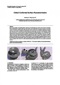
Fig. 3. As the distance between claimed and true location increases so does the difference between resulting hash values.
7.1 Model Validation We first evaluated the path metric and the utility of locality sensitive hashing. As we expect, the further away the claimed location of a node is from its true location, the worst its belief rating. To this end, nodes’ claimed locations are varied with respect to their true location and the behavior of the hash values is observed. Figure 3 illustrates that the further away the claimed location of a node is, the greater the change to its hash value. The figure plots the change in hash value with respect to the change in path “distance”. The x-axis shows the difference between the honest path and dishonest path by computing their “distance” as previously defined — by summing the distances between all the sample points of the 2 paths. For this simulation a network of 50 × 50 was used with a communication radius of 10 and a sampling rate of 100. A node was randomly selected at distance at least d from the sink, d being the width of the network. False locations were acquired by randomly choosing a direction and calculating the coordinates of the new claimed location, based on the magnitude of the claim. The strong linear correlation shows that our distance measure between paths truthfully captures the severity of the wrong location claim. Using hash values, each node along the path forms a belief as to the honesty of the packet that comes its way, by comparing its hash value with the hash values in the history for the region. The beliefs formed will be slightly different for all nodes on the route. Normally the beliefs are stronger near the start of the path because the change in the path is more significant at the earlier nodes than those further away; in other words, since the start nodes are looking at a shorter path the percentage of the claim is greater. Figure 4 shows the actual belief ratings formed by each node along a 6 hop path from source to sink. Values are shown for when the adversary claims to be at positions from 0 to 35 units away from its true location (or 0 to 4 hops as the nodes have a radius of 10) in a network of 50 × 50. As can be seen, the belief quickly drops once the adversary makes a claim more than 1 hop away. ACM Journal Name, Vol. V, No. N, Month 20YY.
Collaborative Location Certification for Sensor Networks
·
17
belief value 0.7 0.6 0.5 0.4 0.3 0.2 0.1 0 0
5 10 15 20 25 30 35 claimed distance
1
2
3
4
5
6
hop #
Fig. 4. The beliefs generated by each node along the path, as the adversary claimed distance increases.
7.2 Parameter Fine-tuning There are a number of parameters used in our protocol that interestingly have little or no effect on the overall belief rating generated. The power of using locality sensitive hashing with history data overwhelms other network factors. We mentioned how the hash function requires a random vector of size 2k where k is the degree of parametrization of the path (“sampling parameter”). Figure 5 shows that even a low sampling parameter will result in quite accurate belief ratings. There is no clear distinction between a value k ranging from 20 to 2000, only the sampling parameter of 10 appears insufficient. This is important, because, by using a lower parametrization we reduce the overhead of the hash function computation. This graph only gives a snapshot of what one node “believes”. A node on the path from source to sink was arbitrarily selected (in this case the node at hop 4) and it’s beliefs were plotted, this being the reason for the routing irregularities seen in the figure. In addition, we have found that network size and density do not noticeably impact the efficacy of our certification system. Again, this is because the hash values give overwhelmingly good indicators as to the honesty of a node, regardless of network specifics. Figure 6 shows belief ratings for three typical network topologies, namely (i) an area of 50 × 50, n = 100, R = 10, deg = 10, (ii) 100 × 100, n = 500, R = 10, deg = 14, (iii) 500 × 500, n = 1000, R = 40, deg = 17 — where n is the number of nodes, R the communication radius and deg the average node degree. The set of simulations indicate a number of interesting observations that are useful for parameter tuning in practice. —For sufficiently good belief ratings, only 5 nodes on the relay path are required to attach their beliefs. This substantially reduces communication overhead and validates the stochastic belief propagation as only a small fraction of nodes need to participate. ACM Journal Name, Vol. V, No. N, Month 20YY.
18
·
Gao, Sion, Lederer 1 10 samples 20 samples 50 samples 100 samples 500 samples 2000 samples
0.9 0.8
belief rating
0.7 0.6 0.5 0.4 0.3 0.2 0.1 0 0
0.5
1
1.5
2 hops
2.5
3
3.5
4
Fig. 5. Belief values (as a function of hop-distance of claimed vs. true location) using various samplings of the paths. This shows that we can reduce the overheads of hash function computation by using a lower parametrization. 0.9 100 nodes 500 nodes 1000 nodes
0.8 0.7 belief rating
0.6 0.5 0.4 0.3 0.2 0.1 0 0
0.5
1
1.5
2
2.5 hops
3
3.5
4
4.5
Fig. 6. Beliefs under generated by the following networks: (i)50 × 50, n = 100, R = 10, (ii) 100 × 100, n = 500, R = 10 (iii) 500 × 500, n = 1000, R = 40
—The number of samples (in hashing) for a path can be as low as 20. —With the above parameters, the belief rating of a packet from a source node that claimed to be at a location as close as a single hop away, decreases quickly toward zero. 7.3 Detection of malicious claims Figure 7 illustrates the percentage of packets accepted by the data sink after examining their belief values and comparing them with a “threshold value” for acceptance. Specifically, the sink will require the average of the lowest 3 beliefs on the path to be above the threshold to be accepted. The graph also shows the percentage of honest nodes accepted (the distance between claimed location and the true location is 0). Having a high threshold of 80% is too strict, and some honest packets ACM Journal Name, Vol. V, No. N, Month 20YY.
Collaborative Location Certification for Sensor Networks
·
19
1 "t10.txt" "t50.txt" "t80.txt"
0.9 0.8 0.7 0.6 0.5 0.4 0.3 0.2 0.1 0 0
20
40
60
80
100
Fig. 7. The percentage of the number of packets accepted by the sink node with respect to distance claim of node in terms of the number of hops away it is from true location. The beliefs received at the sink must be above the given threshold value to be accepted.
are therefore incorrectly dropped. For this simulation we incorporated variability into the routing pattern by having only 85% of the links be active at any given time (thus the routes taken by the packets from the same source vary). The results show that having only a small percentage of nodes attach beliefs is sufficient for a surprisingly strong detection ability. For example, by just having 5 beliefs attached, the detection accuracy is 95%. 8. RELATED WORK Location discovery is a decades-old problem important in all areas where either free-roaming devices are involved (cell phones), or where devices are deployed in an ad-hoc fashion (sensor motes). Localization systems usually involve two phases. (i) Calculating the distance to some other stations whose positions are known. These “stations” may be satellites as used in GPS, or cell towers, or some other devices. In some cases it is sufficient to have the relative distances between devices using a local coordinate system (see [Capkun et al. 2002]), in which case no pre-established positions are needed; rather nodes can fix their there own position as the center of the universe, (0,0), and interpret the location of their peers with respect to themselves. (ii) Combining distance and/or angle data, whereby a node merges measurements from a number of different anchors (normally 3) using triangulation, trilateration, or multi-lateration to pinpoint its exact location. Sometimes a third phase is executed to refine the distance positions. The Iterative Refinement procedure proposed by Savarese et al. [Savarese et al. 2002] has nodes iteratively update their positions. Devices can calculate their position relative to the anchors by sending either an RF, ultrasound, or light signals to their neighbor (or anchor) and calculate there distance to it with one of the following techniques: 1) Received Signal Strength Indicator (RSSI): The receiver measures the strength of an incoming signal, and based on the known power it was transmitted at, the receiver can calculate its distance from the transmitter. The propagation loss is translated into a distance ACM Journal Name, Vol. V, No. N, Month 20YY.
20
·
Gao, Sion, Lederer
estimate. 2) Time of Arrival (ToA) and Time Difference of Arrival (TDoA) the receiver uses the known propagation speed of a signal to calculate its location based on the time it take to receive a signal. 3) Angle of Arrival (AoA) can be used by devices with onmidirectional antennas to determine the angle at which a signal is received. With regard to sensor networks, there is much talk as to whether localization should rely on external systems and hardware, such as GPS, or whether localization should be performed using solely a collaborative effort among the nodes themselves with little or no outside help. The general consensus is that GPS reliance should be avoided primarily because of the cost associated with it. Equipping every mote with a GPS receiver would cost many times over the cost for the entire mote. GPS has other failings too such as its limited efficacy indoors or under tree cover. And, from a theoretical standpoint, a free-standing solution is far more elegant than one that needs the support of outside systems. The advantages and disadvantages of RF vs. ultrasound and ToA vs. AoA are debated in the literature. RF signals for instance do not propagate well in environments with great amounts of metal or other reflective material leading to multipath effects, dead-spots, noise and interference. [Langendoen and Reijers 2003] gives a thorough comparison of the various methods. In addition, localization schemes can be classified into range-dependent and range-independent based schemes. Range-dependent schemes use the ideas mentioned above to calculate distances between nodes (ToA [Capkun et al. 2002], TDoA [Savvides et al. 2001; Priyantha et al. 2000; Hu and Evans 2004; Zhao et al. 2003], AoA [Niculescu and Nath 2003a], or RSSI [Bahl and Padmanabhan 2000; Girod and Estrin 2001]). Attacks and countermeasures for range-dependent schemes have been presented in [Capkun and Hubaux 2005]. In the range-independent localization schemes, nodes determine their location without use of time, angle, or power measurements. Nodes depend on beacons, or connectivity information to compute their location. DV-hop [Nicolescu and Nath 2001], amorphous localization [R. Nagpal 2003], and APIT [He et al. USA] are examples. Centroid [Bulusu et al. 2000], is an outdoor localization scheme, where reference points broadcast beacons with their coordinates, and nodes estimate their position as the centroid of the locations of all the reference points that they hear. Centroid has a very simple implementation and low communication cost. However, it results in a crude approximation of node location. Indoor positioning systems bases on the propagation of sound include Active Bat [Ward et al. 1997] and Cricket [Priyantha et al. 2000]. In [Bahl and Padmanabhan 2000], RSSI is used and signal-to-noise ratio within the building is pre-measured to increase accuracy. Other techniques based on the received signal strength include SpotON [Hightower et al. 2000] and Nibble [Castro et al. 2001]. Positioning algorithms for wireless ad hoc networks are presented in [Doherty et al. 2001], where all the nodes report their distance estimates to a central location which solves an optimization problem of minimizing the error measurements of each node. In [Bulusu et al. 2000], Bulusu, Heidemann and Estrin propose a positioning system based on a set of landmark base stations with known positions. Each node then estimates its position based on its proximity to the base stations. In [Capkun et al. 2002], ACM Journal Name, Vol. V, No. N, Month 20YY.
Collaborative Location Certification for Sensor Networks
·
21
Capkun, Hamdi and Hubaux present a GPS-free positioning system in which each node computes the position of its neighbors in its local coordinate system, and then the nodes agree on the center and direction of the network coordinate system by a collaborative action. Niculescu and Nath [Niculescu and Nath 2003b] present a distributed ad hoc positioning system that works as an extension of both distance vector routing and GPS positioning, in order to provide approximate positions for all nodes in a network where only a limited fraction of nodes have self-positioning capabilities. In [Niculescu and Nath 2003a], the same authors present an ad hoc network positioning system based on the angle of arrival technique. In [Savvides et al. 2001] Savvides, Han and Srivastava propose a dynamic fine-grained localization scheme for sensor networks in which groups of nodes collaborate to resolve their positions by solving nonlinear systems whose sizes depend on the sizes of the groups. Basu et al. [Basu et al. 2006] are concerned with noisy distance and angle measurements. [Moore et al. 2004] also deals with noisy range measurements without GPS by formulating the localization problem as a two-dimensional graph realization problem: given a planar graph with approximately known edge lengths, recover the Euclidean position of each vertex up to a global rotation and translation. The secure localization problem has been studied by a number of groups. For example, the SeRLoc protocol [Lazos and Poovendran 2004] tackles secure localization by using specially equipped “locator” nodes that emit powerful beacon signals through the networks. Depending on the beacons a node hears, it computes the “center of gravity” of the overlapping regions to determine its location. The locator devices are tamper proof. In another protocol, robust statistics are used to improve the vigorousness of an anchor-based localization algorithm in a hostile environment where the nodes may receive false information from the neighbors [Li et al. 2005]. Even though nodes can obtain their locations correctly by these secure localization protocols or extra secure location support such as GPS, these do not prevent a node from lying about its location and generating event reports with a false location claim. Our primary focus in this paper is the problem of location verification, which verifies whether a location claim is truthful, and further, whether packets with a location claim are honest. In the literature a number of protocols have been proposed by using fine grained timing analysis. Capkun and Hubaux [Capkun and Hubaux 2004; 2005] introduced Verifiable Multilateration (VM), to prevent a node from lying about its own position, and Verifiable Time Difference of Arrival (VTDOA), to stop an adversary from influencing the reported position of a true node. VM uses 3 anchor nodes that surround the unknown node. Transmissions are with RF signals that travel at the speed of light, therefore claimant can only pretend to be further away from any one anchor, but not closer (since it can’t make its transmissions go faster than light). So, to pretend a greater distance to one anchor node, it must claim a small distance to another node, which is impossible since trilateration is used. VTDOA compares the TDOA and ToF distance estimations to prevent a malicious node from jamming the signal of a true node and replaying it from another location. Technique requires that the anchor nodes are synchronized with each other (and the claimant node). The Echo [Sastry et al. 2003] protocol uses a multi-part handshake between some ACM Journal Name, Vol. V, No. N, Month 20YY.
22
·
Gao, Sion, Lederer
“verifying” nodes and the claimant using RF and ultrasound to guarantee that the node is in an asserted area. It does not however pinpoint the precise location of a node, it only verifies that it is within a rough region, and it requires that the verifiers be within the region in question. Waters and Felten [Waters and Felten 2003] present a similar scheme which uses tamper-resistant devices. Timing analysis typically requires highly accurate clocks that may not be realistic in networks with inexpensive hardware, e.g., cheap sensor nodes. For example, the VM scheme requires accurate synchronization (maximum clock difference of 1ns) [Capkun and Hubaux 2004; 2005]. The use of ultrasound relaxes a little the stringent requirement on synchronization, but requires additional hardware artifact. In addition, these anchor-based schemes typically assume authorized and trustworthy anchor nodes and often require a sufficient number of anchors that cover all the sensor nodes, which may not be practical when the deployment and the operation of the sensor network are in hostile territory. Moreover, the scheme we propose here does not assume any anchor nodes, nor any special hardware such as ultrasound transmitters. We take a different approach and establish, by the participation of all the sensor nodes, a collaborative community that certifies the locations of packets routed through the network. We can thus make use of the traffic pattern, brought by the message relaying, at little extra cost. The challenge resides in what and how each sensor node participates in the job of certifying the truthfulness of a location claim from a packet and keeping a low cost of doing so. The scheme we propose here does not assume any anchor nodes, nor any special hardware such as ultrasound transmitters. We take a different approach and establish, by the participation of all the sensor nodes, a collaborative community that certifies the locations of packets routed through the network. We can thus make use of the traffic pattern, brought by the message relaying, at little or no extra cost. 9. CONCLUSION AND FUTURE WORK In this paper we have introduced a collaborative location certification scheme that determines whether nodes are falsely claiming incorrect locations in their event reports to the sink. Experiments have shown that with low overhead this scheme can detect incorrect location claims as close as one hop away from the node’s true location. In future work we believe it is important to explore how our protocol can be applied to detect, in general, anomalous routing behavior. By using history data to compare traffic patterns we can detect whether the network is under a wormhole or sinkhole attack. Moreover, we believe significant elegance and additional features can be achieved by deploying asymmetric key crypto. Specifically, we would like to investigate if low-overhead asymmetric key cryptography can be deployed to construct homomorphisms that will allow in-network location claim evaluation to optimize network utilization and overall consumption by dropping malicious traffic. REFERENCES Bahl, P. and Padmanabhan, V. 2000. Adar: An in-building rf-based user location and tracking system. In In Proc. of the IEEE INFOCOM 2000. Tel-Aviv, Israel. Basu, A., Gao, J., Mitchell, J. S. B., and Sabhnani, G. 2006. Distributed localization using ACM Journal Name, Vol. V, No. N, Month 20YY.
Collaborative Location Certification for Sensor Networks
·
23
noisy distance and angle information. In MobiHoc ’06: Proceedings of the seventh ACM international symposium on Mobile ad hoc networking and computing. ACM Press, New York, NY, USA, 262–273. Bulusu, N., Heidemann, J., and Estrin, D. 2000. Gps-less low cost outdoor localization for very small devices. In In IEEE Personal Communications Magazine. C . amtepe, S. A. and Yener, B. 2005. Key distribution mechanisms for wireless sensor networks: a survey. Tech. Rep. TR-05-07, Rensselaer Polytechnic Institute. March. Capkun, S., Hamdi, M., and Hubaux, J.-P. 2002. GPS-free positioning in mobile ad hoc networks. Cluster Computing 5, 2, 157–167. Capkun, S. and Hubaux, J.-P. 2004. Securing position and distance verification in wireless networks. Tech. Rep. EPFL/IC/2004-43. Capkun, S. and Hubaux, J. P. 2005. Secure positioning of wireless devices with application to sensor networks. In Proceedings of Infocom. Miami, FL, USA. Castro, P., Chiu, P., Kremenek, T., and Muntz., R. 2001. A probabilistic location service for wireless network environments. In Ubiquitous Computing. Cheung, S., Dutertre, B., and Lindqvist, U. 2005. Detecting denial-of-service attacks against wireless sensor networks. Tech. Rep. Technical Report SRI-CSL-05-01, Computer Science Laboratory, SRI International. May. Datar, M., Immorlica, N., Indyk, P., and Mirrokni, V. S. 2004. Locality-sensitive hashing scheme based on p-stable distributions. In SCG ’04: Proceedings of the twentieth annual symposium on Computational geometry. ACM Press, New York, NY, USA, 253–262. Doherty, L., Pister, K., and Ghaoui, L. E. 2001. Convex position estimation in wireless sensor networks. In In Proceedings of Infocom. Girod, L. and Estrin, D. 2001. Robust range estimation using acoustic and multimodal sensing. In In IEEE/RSJ Int. Conf. on Intelligent Robots and Systems (IROS). Goldreich, O. 2001. Foundations of Cryptography. Cambridge University Press. He, T., Huang, C., Blum, B., Stankovic, J., and Abdelzaher, T. San Diego, CA, USA. Rangefree localization schemes in large scale sensor network. In In Proc. of MOBICOM 2003. 2003. Hightower, J., Boriello, G., and Want, R. 2000. Spoton: An indoor 3d location sensing technology based on rf signal strength. In Technical Report 2000-02-02. University of Washington. Hu, L. and Evans, D. 2004. Localization for mobile sensor networks. In MobiCom ’04: Proceedings of the 10th annual international conference on Mobile computing and networking. ACM Press, New York, NY, USA, 45–57. Hu, Y. C., Perrig, A., and Johnson, D. 2003. Packet leashes: a defense against wormhole attacks in wireless networks. In INFOCOM. Indyk, P. and Motwani, R. 1998. Approximate nearest neighbors: towards removing the curse of dimensionality. In STOC ’98: Proceedings of the thirtieth annual ACM symposium on Theory of computing. ACM Press, New York, NY, USA, 604–613. Intanagonwiwat, C., Govindan, R., and Estrin, D. 2000. Directed diffusion: a scalable and robust communication paradigm for sensor networks. 56–67. Karlof, C. and Wagner, D. 2003. Secure routing in wireless sensor networks: Attacks and countermeasures. Elsevier’s AdHoc Networks Journal, Special Issue on Sensor Network Applications and Protocols 1, 2–3 (September), 293–315. Karp, B. and Kung, H. T. 2000. GPSR: greedy perimeter stateless routing for wireless networks. In MobiCom ’00: Proceedings of the 6th annual international conference on Mobile computing and networking. ACM Press, New York, NY, USA, 243–254. Langendoen, K. and Reijers, N. 2003. Distributed localization in wireless sensor networks: a quantitative comparison. Comput. Networks 43, 4, 499–518. Lazos, L. and Poovendran, R. 2004. SeRLoc: secure range-independent localization for wireless sensor networks. In WiSe ’04: Proceedings of the 2004 ACM workshop on Wireless security. ACM Press, New York, NY, USA, 21–30. ACM Journal Name, Vol. V, No. N, Month 20YY.
24
·
Gao, Sion, Lederer
Li, Z., Trappe, W., Zhang, Y., and Nath, B. 2005. Robust statistical methods for securing wireless localization in sensor networks. In Proceedings of the Fourth International Symposium on Information Processing in Sensor Networks. 91–98. Moore, D., Leonard, J., Rus, D., and Teller, S. 2004. Robust distributed network localization with noisy range measurements. In SenSys ’04: Proceedings of the 2nd international conference on Embedded networked sensor systems. ACM Press, New York, NY, USA, 50–61. Nicolescu, D. and Nath, B. 2001. Ad-hoc positioning systems (aps). In In Proc. of IEEE GLOBECOM 2001. San Antonio, TX, USA. Niculescu, D. and Nath, B. 2003a. Ad hoc positioning system (aps) using aoa. In In Proc. of INFOCOM. Francisco, CA, USA. Niculescu, D. and Nath, B. 2003b. Dv based positioning in ad hoc networks. In Kluwer journal of Telecommunication Systems. 267–280. Papadimitratos, P. and Haas, Z. J. 2002. Secure routing for mobile ad hoc networks. In SCS Communication Networks and Distributed Systems Modeling and Simulation Conference (CNDS 2002). Priyantha, N., Chakraborthy, A., and Balakrishnan, H. 2000. The cricket location-support system. In In Proc. of MOBICOM. Boston, MA, USA. R. Nagpal, H. Shrobe, J. B. 2003. Organizing a global coordinate system from local information on an ad hoc sensor network. In In Proc. of IPSN 2003. Palo Alto, USA. Sanzgiri, K., Dahill, B., Levine, B., and Belding-Royer, E. 2002. A secure routing protocol for ad hoc networks. In International Conference on Network Protocols (ICNP). Sastry, N., Shankar, U., and Wagner, D. 2003. Secure verification of location claims. In In Proc. of WISE 2003. Savarese, C., Rabaey, J. M., and Langendoen, K. 2002. Robust positioning algorithms for distributed ad-hoc wireless sensor networks. In Proceedings of the General Track: 2002 USENIX Annual Technical Conference. USENIX Association, Berkeley, CA, USA, 317–327. Savvides, A., Han, C.-C., and Strivastava, M. B. 2001. Dynamic fine-grained localization in ad-hoc networks of sensors. In MobiCom ’01: Proceedings of the 7th annual international conference on Mobile computing and networking. ACM Press, New York, NY, USA, 166–179. Ward, A., Jones, A., and Hopper, A. 1997. A new location technique for the active office. In IEEE Personal Communications Magazine. Waters, B. and Felten, E. 2003. Secure, private proofs of location. Tech. Rep. TR-667-03, Princeton University. January. Wood, A. D. and Stankovic, J. A. 2002. Denial of service in sensor networks. IEEE Computer 35, 10, 54–62. Ye, F., Zhong, G., Cheng, J., Lu, S., and Zhang, L. 2003. PEAS: A robust energy conserving protocol for long-lived sensor networks. In ICDCS ’03: Proceedings of the 23rd International Conference on Distributed Computing Systems. IEEE Computer Society, Washington, DC, USA, 28. Zhao, F., Liu, J., Huang, Q., and Zou, Y. 2003. Fast and incremental node localization in ad hoc networks. Zhou, G., He, T., Krishnamurthy, S., and Stankovic, J. A. 2004. Impact of radio irregularity on wireless sensor networks. In MobiSys ’04: Proceedings of the 2nd international conference on Mobile systems, applications, and services. ACM Press, New York, NY, USA, 125–138.
ACM Journal Name, Vol. V, No. N, Month 20YY.