fundamental problem: can the network geometry be recon- structed using .... The boundary of R is denoted as âR and may have multiple cycles. The inner medial ... Left: The Voronoi graph (shown in dashed lines) and the Delaunay complex for a set .... Lipschitz function (by triangle inequality, proof omitted). That is, ILFS(x) ...
Connectivity-based Sensor Network Localization with Incremental Delaunay Refinement Method Yue Wang∗
Sol Lederer∗
Jie Gao∗
∗ Department of Computer Science, Stony Brook University. {yuewang, lederer, jgao}@cs.sunysb.edu
Abstract—We study the anchor-free localization problem for a large-scale sensor network with a complex shape, knowing network connectivity information only. The main idea follows from our previous work [19] in which a subset of the nodes are selected as landmarks and the sensor field is partitioned into Voronoi cells with all the nodes closest to the same landmark grouped into the same cell. We extract the combinatorial Delaunay complex as the dual complex of the landmark Voronoi diagram and embed the combinatorial Delaunay complex as a structural skeleton. In this paper we develop a new landmark selection algorithm with incremental Delaunay refinement method. This algorithm does not assume any knowledge of the network boundary and runs in a distributed manner to select landmarks incrementally until both the global rigidity property (the Delaunay complex is globally rigid and thus can be embedded uniquely) and the coverage property (every node is not far from the embedded Delaunay complex) are met. The new algorithm substantially improves the robustness and applicability of the original localization algorithm, especially in networks with very low average degree (even nonrigid networks) and complex shapes.
I. I NTRODUCTION The location of sensor nodes is an indispensable component for both network operation and sensor data integrity. In this paper we study the network localization problem for a largescale sensor network with a complex shape. We do not assume any anchor nodes with known locations and use only network connectivity information to recover the relative positioning of all the nodes. Thus we require no extra hardware supplements (e.g., for angle or distance measurements) and investigate a fundamental problem: can the network geometry be reconstructed using network connectivity alone? This is a simple yet very challenging setting for network localization. A major challenge in anchor-free localization is to handle possible flip ambiguities. Two triangles sharing an edge can be embedded in two possible ways, with the two triangles on the same side, or on opposite sides of the common edge. In general, whether a graph has a unique embedding or not is investigated in graph rigidity theory [16]. A graph is rigid in 2D if a realization of the graph in the plane cannot be continuously deformed without changing the lengths of the edges. A graph is globally rigid if it has a unique embedding in the plane given the edge lengths. Graph rigidity in 2D has been relatively well understood. Both a combinatorial characterization of globally rigid graphs and polynomial algorithms for testing such graphs are known [6], [17]. It is however not trivial to apply these rigidity results in the development of efficient localization algorithms. Given a graph with the edge lengths specified, finding a valid graph realization in Rd for a fixed dimension
d is an NP-complete problem [4], [5], [23]. Even if we know that a graph is globally rigid in 2D, there is no known efficient algorithm to find the realization of the graph with the given edge lengths. The pioneer work of using rigidity theory in network localization [3], [7], [9], [14], [15], [20], [25] focuses on identifying special graphs that do admit efficient localization algorithms. The first idea is to use trilateration graphs [9], [14], [15], [20]. A trilateration graph is defined recursively. It is either a triangle or a trilateration graph with a trilateration extension, defined as adding an additional vertex with three edges to existing vertices. If the network contains a trilateration graph, one can exhaustively search for the ‘seed’ triangle in the graph and greedily find the trilateration extensions. Thus an incremental algorithm can be adopted to find the realization of the network. A trilateration graph is a stronger condition than global rigidity (i.e., there are globally rigid graphs that are not trilateration graphs), and thus may require more edges than necessary to uniquely embed the graph. The second idea is to examine duniquely localizable graphs. A graph with known edge lengths is called uniquely d-localizable if there is a unique realization of the graph in Rd and there is no non-trivial realization in Rk with k > d. For example, a generic simplex of d+1 vertices is uniquely d-localizable. For uniquely d-localizable graphs, So and Ye [7], [25] have shown that a semi-definite program is able to find the realization. It is not known whether d-localizability is a generic property and it is not clear whether there is a combinatorial characterization of graphs that are d-localizable. Both approaches require that the network has sufficiently many edges to be globally rigid. The work in this paper is a follow-up of our previous work [19] in which we proposed a framework for connectivitybased anchor-free localization with a different approach. We select some sensor nodes as landmarks and compute the Voronoi diagram with all the nodes closest to the same landmark grouped into the same Voronoi cell. We extract the combinatorial Delaunay complex1 as the dual complex of the landmark Voronoi diagram – there is a Delaunay edge (or in general a k-simplex) between two (or k) landmarks if their Voronoi cells share some common nodes. In contrast with the previous rigidity work on graphs, we focus on the global rigidity property of the combinatorial Delaunay 1 The Delaunay complex is defined in the notion of abstract simplicial complex [8]. A set α is an (abstract) simplex with dimension dim α = card α−1, i.e., the number of elements in α minus 1. A finite system A of finite sets is an abstract simplicial complex if α ∈ A and β ⊆ α implies β ∈ A.
2
complex, that has high-order topological structures (such as Delaunay triangles) compared with graphs that do not (having only vertices and edges). The combinatorial Delaunay complex may be globally rigid when the combinatorial Delaunay graph is not. See Figure 1 for an illustration. As opposed to the u
p
p
u
u
w
w v
v
w v
p
Fig. 1. Two Delaunay triangles △uvw and △uvp sharing an edge. The first figure is the only valid embedding, for in a simplicial complex two simplices can only intersect at a common face. The graph is not globally rigid.
graph rigidity approaches discussed earlier, this approach does not explicitly require that the network to be embedded is globally rigid. This sheds some light on providing reasonable localization results when the network has low node density (even uniformly sparse but non-rigid graphs such as a gridlike network with punched holes). In [19] we proposed an algorithm for landmark selection to guarantee that the generated combinatorial Delaunay complex is globally rigid and admits a unique realization in the plane. This leads to an algorithm to put together the Delaunay triangles in an incremental manner which helps localize the rest of the nodes in the network. The algorithm for selecting landmarks first uses a boundary detection algorithm [10]– [13], [18], [26] to identify the network boundary nodes and then selects the landmarks to be a γ-sample with γ < 1. Specifically, every boundary node has a landmark within its inner local feature size, defined as the distance to the closest node on the medial axis (which is the collection of nodes with two or more closest nodes on the boundary). More details on this algorithm and comparison to our new algorithm in this paper will be further explained in the next section. The dependency on the boundary detection algorithm puts limitations on the applicability of the localization algorithm as in the case of extremely low density networks, where boundary detection algorithms do not work well. Examples of some of these cases were shown in [19]. The main contribution in this paper is an incremental landmark selection algorithm that does not assume knowledge of the network boundary. In particular, we start with no knowledge of the network topology (whether there are holes or how many there are, etc.) and develop local conditions to test whether a node should be included as a new landmark. The landmarks selected naturally adapt to the local geometry of the network, with a higher density of landmark nodes selected in regions with more detailed and complex features. This new landmark selection algorithm greatly enhances the robustness of our algorithm in cases of extremely sparse or even non-rigid networks, or networks with very complicated shapes that are challenging for boundary detection algorithms. We are not aware of any other localization algorithms using only connectivity information with comparable performance. We demonstrate the improved performance of our algorithm in various network settings in the simulation section.
II. L OCALIZATION B Y D ELAUNAY C OMPLEX In this section we use a continuous setting to go though the framework of network localization by the combinatorial Delaunay complex and provide the theoretical foundation of the incremental Delaunay refinement algorithm. The algorithm implementation in the network setting is elaborated on in the next section. The sensor field is assumed to be a continuous domain R ∈ R2 with perhaps some interior holes. For any two points p, q ∈ R, we denote by |pq| their Euclidean distance and d(p, q) the geodesic distance (shortest path distance) between them inside R. The geodesic distance is an analog of the minimum hop count distance in the discrete setting. A ball centered at a point p of radius r, denoted by Br (p), contains all the points within geodesic distance r from p. The boundary of R is denoted as ∂R and may have multiple cycles. The inner medial axis of R is the collection of points in R that have two or more closest points on the boundary ∂R. The inner local feature size of a point p ∈ ∂R, denoted by ILF S(p), is the distance from p to the inner medial axis of R. A set of landmarks L on the boundary ∂R is called a γ-sample2 if for any point p ∈ ∂R, there is at least one landmark within distance γ · ILF S(p) from p. Suppose L is a set of landmarks on the domain boundary ∂R, the Voronoi cell of a landmark u, denoted as V (u), includes all the points that have u as a closest landmark: V (u) = {p ∈ R | d(p, u) ≤ d(p, v), ∀v ∈ L, v 6= u}. The collection of Voronoi cells is denoted as the landmark Voronoi diagram V (L) for the set L of landmarks. A point is called a Voronoi vertex if it has equal distance to at least three landmarks. The Voronoi vertices inside R are called the inner Voronoi vertices. A ball Br (p) centered at an inner Voronoi vertex p with radius r equivalent to the distance from p to the closest landmarks is called a Voronoi ball.
∂R
Fig. 2. Left: The Voronoi graph (shown in dashed lines) and the Delaunay complex for a set of landmarks on the boundary ∂R. The Delaunay simplices (vertices, edges, triangles, tetrahedrons) are shaded. Right: The union of Voronoi balls approximately covers the domain R.
The combinatorial Delaunay complex of the landmarks L, denoted by DC(L), is the collection of sets DC(L) = {α ⊆ L | ∩u∈α V (u) 6= ∅}. In other words, a set α ⊆ S is a Delaunay simplex if the intersection of the Voronoi cells of landmarks of α is nonempty. The Delaunay complex has naturally 0-dimensional 2 Notice that the definition of γ-sample is different from the typical definition in geometric processing [1], [2] where the local feature size is used. The medial axis for a domain R has two parts, one inside R and one outside R. For our setting we do not have access to the part of the medial axis outside of R and we can only use the inner local feature size.
3
simplices such as the landmarks, 1-dimensional simplices such as Delaunay edges, and 2-dimensional simplices such as Delaunay triangles, and possibly higher order simplices such as tetrahedrons. See Figure 2 for an example. A. γ-sample, rigidity and coverage In our previous work [19], we show a framework for network localization by embedding the Delaunay complex DC(L) extracted from the network connectivity. The main result in [19] is a proof that when the landmarks are selected as a γ-sample of the domain R with γ < 1, the Delaunay complex DC(L) is globally rigid and thus admits a unique realization in the plane. This establishes the foundation of the localization algorithm as we can now embed the Delaunay complex incrementally and then localize the entire network with the Delaunay complex as a structural skeleton. For localization, we also want that the Delaunay complex provides good ‘coverage’ of the sensor field in the sense that every node is not very far from the Delaunay complex, so that the Delaunay complex faithfully represents the network shape. In particular, we take B to denote the union of all the Voronoi balls, and U the shape of the union of these balls. As we will prove later, the γ-sample guarantees that the union of Voronoi balls is a good approximation of R and the approximation is improved as the density of landmarks increases. See Figure 2 (ii) for an example. Rigorously, we define that the Delaunay complex DC(L) δ-covers R if every point x ∈ R will be within distance (1 + δ) · r from the center p of a Voronoi ball Br (p), where r is the radius of this Voronoi ball. Using the union of the Voronoi balls to approximate the shape R was initially proposed in geometric processing and computer graphics [2]. It has been shown that the errors in the position and normal of the surface of U with R is bounded everywhere, given sufficiently dense samples on the ∂R. However, we cannot directly apply the results in [2] as there are a couple of differences with our setting. First, the metric we are working with is the geodesic shortest path metric, instead of the Euclidean metric used in [2]. In addition, as we only have sensors in the interior of R, we do not have access to the part of medial axis that is outside R and we are only able to use the inner local feature size to define the γ-sample. Before we prove the coverage theorem, let us first understand the boundary of the union of balls U. The boundary of U contains some circular arcs from the balls in B. We first characterize what arc can possibly stay on the boundary of U. Each Voronoi edge in V (L) has two endpoints, being either a Voronoi vertex or a point on the boundary ∂R. A Voronoi edge with two Voronoi vertex endpoints is called an inner edge. A Voronoi edge with two endpoints on the boundary is called an outer edge. A Voronoi edge with both a Voronoi vertex and a point on the boundary is called a mixed edge. For each Voronoi ball B, the three landmarks partition its boundary ∂B into three circular arcs. We label the arc between two landmarks u, v with the label of the Voronoi edge of u, v as either inner, outer, or mixed. We now claim that only mixed
arcs can possibly appear on ∂U. First realize that the interior points of an inner arc cannot stay on the boundary of U, since the arc is enclosed inside the union of the two Voronoi balls that go through u, v. Second if we choose γ < 1, then the Voronoi diagram inside R is connected as proved in Corollary 2.10 in [19]. Thus there cannot be an outer edge in V (L), since this edge will be disconnected from the rest of the Voronoi diagram. Now for a Voronoi ball Br (p) with a mixed edge between landmarks u, v we define a pie as the set of points in R bounded by the boundary segment between u, v and the shortest paths from p to u, v. Only the points inside a pie with a mixed arc can possibly stay outside U. See Figure 3. Notice that in the case of a degeneracy, a Voronoi ball can have four or more landmarks. The classification of edges and the proof later are the same in that case. Theorem 2.1. For a connected region R ⊆ R2 , we select landmarks L as a γ -sample on the region boundary ∂R with γ < 1. Then the Delaunay complex δ -covers R, with δ = 2γ/(1 − γ). Proof: We first prove the claim for points on ∂R. Consider a point x on ∂R in between two landmarks u, v, as shown in Figure 3. Lemma 2.8 in [19] says that there is a p Voronoi vertex p with u, v as r two closest landmarks and the y Voronoi edge with respect to u, v u v is a mixed edge. Without loss x of generality we assume that x’s Fig. 3. Any x is within distance closest landmark is u. By the γ- δ · r from a Voronoi ball. A pie ˆ is shown sample property, d(u, x) ≤ γ · between a mixed arc uv in shade. ILF S(x). Now we assume by contradiction that d(p, x) > (1 + δ)r. Thus γ · IF LS(x) ≥ d(u, x) ≥ d(p, x) − d(p, u) > (1 + δ)r − r = δr by the triangle inequality. Thus ILF S(x) > δr/γ. We also know that the inner local feature size is a 1Lipschitz function (by triangle inequality, proof omitted). That is, ILF S(x) ≤ ILF S(u) + d(u, x). As we know that the Voronoi ball Br (p) touches three landmarks and contains at least one point on the medial axis in R, ILF S(u) ≤ 2r. Thus we have, ILF S(x) ≤ 2r + γ · ILF S(x). Combining the inequalities, we have δr/γ < IF LS(x) ≤ 2r/(1 − γ). That gives us δ < 2γ/(1 − γ), a contradiction. If the claim is true for all points on ∂R, it is true for all points in R. Suppose otherwise, then there is a point y in the interior of R that is not δ-covered. y can only possibly stay inside a pie, as shown in Figure 3. Then there must be another point x ∈ ∂R such that y stays on the geodesic shortest path from p to x. Thus y is covered by Br (p), the same Voronoi ball that covers x. B. Landmark selection for both rigidity and coverage Based on the previous discussion, there are two desirable criteria, namely, global rigidity and coverage, for the final Delaunay complex. In this subsection we investigate local
4
conditions for landmark selection to guarantee both rigidity and good coverage of the induced Delaunay complex: 1) Local Voronoi edge connectivity: The Voronoi edges for each landmark u form a connected set. 2) Local Voronoi ball coverage: Each node x inside a Voronoi cell V (u) is δ-covered by a Voronoi ball Br (p), where p is a Voronoi vertex with landmark u. We first show that if both conditions are satisfied for a set of landmarks L, then the Delaunay complex DC(L) satisfies both the global rigidity and coverage property. This is relatively straightforward. After this, we examine how to design a landmark selection algorithm to meet these conditions. 1) Rigidity of the Delaunay complex: When the local Voronoi edge connectivity condition is met, we argue that the Delaunay complex is globally rigid. To do that, we will make use of a theorem proved in [19]:
is sensitive to noise. New landmarks in different Voronoi cells can be inserted in parallel as the algorithm executes locally inside each Voronoi cell. Thus the new landmark selection method is more robust and practical compared with the γsampling used in our previous algorithm. Of course when the algorithm terminates, it produces a set of landmarks L so that the Delaunay complex DC(L) has both the global rigidity and the coverage property. Next, we show the algorithm terminates and has bounded landmark density. 4) Landmark density by incremental refinement: Here we show that every landmark q added by the incremental algorithm is not sufficiently covered by existing landmarks, i.e., the distance to its closest landmark is at least γ · ILF S(q) for an appropriate parameter γ < 1/3. If a point x ∈ ∂R is within γ · ILF S(x) from any landmark, we say x is γ-covered. We first state a useful Lemma.
Theorem 2.2. [Global Rigidity] If V (L) is connected inside R, the Delaunay complex DC(L) is globally rigid.
Lemma 2.3. [Lemma 6.1 in [19]] Given a disk B containing at least two points on ∂R, for each connected component of B ∩ R, either it contains a point on the inner medial axis, or its intersection with ∂R is connected.
The local Voronoi edge connectivity immediately implies the global Voronoi edge connectivity. If otherwise, there must be one landmark whose Voronoi edges have two or more connected components, since the union of all the Voronoi cells is R. Thus the local Voronoi edge connectivity condition implies the global rigidity of DC(L). 2) Coverage of the Delaunay complex: If the local Voronoi ball coverage condition is met for every Voronoi cell, then the coverage property of the Delaunay complex follows directly. 3) Incremental Delaunay refinement algorithm: Since both conditions can be tested locally, we naturally have the following incremental landmark selection algorithm: for each Voronoi cell V (u), 1) If the first condition is not met, the Voronoi edges with u have two or more connected components. Since each Voronoi edge has either a Voronoi vertex or a point on ∂R as endpoints, we select, among all the endpoints of Voronoi edges of u on ∂R, the one that is furthest from u as a new landmark. 2) If the first condition is met, we check the second condition. Among all the points that violate the local Voronoi ball coverage condition, we select the one that is least covered as a new landmark: maxx minBr (p) {δ ′ |d(x, p) = (1 + δ ′ )r}. That is, for each such point x, we choose the Voronoi ball Br (p) with p such that d(x, p) = (1 + δ ′ )r with smallest possible δ ′ . And we select the point x with the largest such δ ′ . This landmark selection algorithm always selects landmarks on the network boundary3 but it does not require the detection of the network boundary, nor does it require the knowledge of the medial axis and local feature size, whose computation 3 Landmarks added by condition 1 will be on ∂R for sure. For the landmarks added by the 2nd condition, by the same argument as in Theorem 2.1 the points outside the Voronoi balls must be inside the pies. And the least uncovered point stays on the region boundary ∂R.
Lemma 2.4. If a Voronoi cell V (u) violates the local Voronoi edge connectivity condition, the new landmark q selected is not covered by any landmark within γ · ILF S(q), for any γ < 1/3. Proof: Since the boundary of the Voronoi cell V (u) is composed of segments on ∂R and the Voronoi edges u, V (u) must have two or more connected components on the domain boundary ∂R as well. Take a Voronoi edge endpoint p that stays on a different boundary segment with u. d(u, p) ≤ d(u, q) since q is the furthest such endpoint. See Figure 4. We take a ball Br (p) with r = d(u, p). Br (p) intersects the boundp ary ∂R in two or more connected q pieces, since both u and p are inside. r By Lemma 2.3 there is a point on the inner medial axis inside Br (p). That u means ILF S(p) < d(u, p). Since IF LS is 1-Lipschitz, ILF S(u) ≤ IF LS(p) + d(u, p) < 2d(u, p). Ap- Fig. 4. The new landmark q is not γ-covered for γ < ply this again we get ILF S(q) ≤ 1/3. IF LS(u)+d(u, q) < 3d(u, q). Thus the claim is proved. Lemma 2.5. If a Voronoi cell V (u) for a landmark u violates the local Voronoi ball coverage condition, the new landmark q selected is not covered by any landmark within γ · ILF S(q), γ = δ/(2 + δ). Proof: If q is selected as the new landmark, d(u, q) > (1 + δ)r for any Voronoi vertex p of the landmark u, r = d(p, u) is the radius of the Voronoi ball at p. Now we have by triangle inequality d(q, u) ≥ d(p, q) − d(p, u) > δr. That is, r < d(q, u)/δ. Similar to the argument in Theorem 2.1, ILF S(q) ≤ d(q, u) + 2r < (1 + 2/δ)d(q, u). Thus, d(q, u) > γ · ILF S(q) with γ = δ/(2 + δ). The above results show that our local conditions do identify
5
points on the boundary that need to be γ-covered for γ < 1/3. If the inner local feature size for any point x ∈ ∂R is at least ε for some fixed ε, then the incremental Delaunay refinement algorithm will eventually terminate, as every new landmark included covers at least an interval of length 2ε centered at itself. This procedure cannot go on indefinitely. We remark that the algorithm will certainly terminate when the landmark set is a γ-sample for any γ < 1, but it may also terminate before that p if both the rigidity and coverage conr ditions are met, as shown in Figure 5. This can be understood in terms of u v our algorithm picking up the major geometric features and ignoring the Fig. 5. The landmark set noisy features of R. The rigidity and may not be a γ-sample of The local feature size coverage properties guarantee that ∂R. for points on the segments the reconstructed Delaunay complex between u, v is smaller than will approximate R and are what we the distance to u or v. really care about in our localization algorithm. The γ-sample for R can be much denser than what is needed in practice. Last we show that the landmark set generated by the incremental algorithm has bounded density. Theorem 2.6. Suppose L is the generated landmark set by the incremental algorithm. If any landmark from L is removed, then it is not a γ ′ -sample of ∂R, with γ ′ = γ/(1 + γ), γ < max(1/3, δ/(2 + δ)). Proof: For the last landmark q inserted, by Lemma 2.4 and Lemma 2.5, it is not within distance γ · ILF S(q) of any existing landmark. Since γ > γ ′ the claim is true for q. For any landmark q ′ added before q, we know d(q, q ′ ) > γ · ILF S(q), since q is added with q ′ already present in the current landmark set. Since IF LS is 1-Lipschitz, we have IF LS(q ′ ) ≤ IF LS(q) + d(q, q ′ ) < (1 + 1/γ) · d(q, q ′ ). Therefore, d(q, q ′ ) > γ ′ · IF LS(q). Notice that this argument is true for any pair of landmarks q, q ′ with q added after q ′ . Thus for q ′ , the distance to any landmark in L is at least greater than γ ′ · IF LS(q ′ ). The claim is true. III. I NCREMENTAL D ELAUNAY R EFINEMENT A. Algorithm description Suppose a large number of sensor nodes are scattered in a geometric region, where nearby nodes can directly communicate with each other. Similar to our previous work [19], we do not enforce that the communication graph follows the unit disk graph model (in our simulations we use both a quasi-UDG model and a probabilistic radio model), nor do we assume any knowledge of the node locations or inter-distances. Our goal is to discover the location of the nodes in the sensor field, using the local connectivity information alone. The basic idea is to select landmarks incrementally in the network until both the global rigidity and the coverage property are satisfied as described in Section II. The biggest difference between this paper and our previous one is that the new landmark selection algorithm does not depend on
the success of boundary detection or the knowledge of the local feature size. Thus the new algorithm is more robust in practice, and yet still captures the geometry of the network. Next we will explain each step of the algorithm in detail. Unless specified otherwise, all the distances are by default measured by the geodesic distance, which is approximated by the minimum hop count between two nodes. 1) Select initial landmarks: We start with two landmarks arbitrarily selected on the boundary. In order to guarantee these two starting landmarks are definitely on the boundary, we flood the network from a random node r and find the farthest node p from r, p must be on the network boundary. Then we flood from p and find the farthest node q from p. q will be on the boundary as well. We use p and q as our two initial landmarks. See Figure 6(i) 2) Compute Voronoi diagram: Once we have some landmarks, we calculate the landmark Voronoi diagram in a distributed way. Each landmark learns of its closest landmark(s) and all the nodes with the same closest landmark are naturally classified to be in the same Voronoi cell. Recall that the landmarks are included incrementally. A new landmark initiates a flood message which is propagated only inside its Voronoi cell—when a node receiving this message sees that its hop count to some preexisting landmark is equal or smaller, then the message is dropped. As more landmarks are included, the size of Voronoi cells decreases, and so does the communication cost. Nodes with more than one closest landmarks lie on a Voronoi edge or vertex. Although the straightforward definition of Voronoi vertex is a node with equal distance to at least three landmarks, one robustness concern is that there may not be a node that qualifies for this definition by the discrete network hop count measure. In [19] we proposed a merging heuristic to get Voronoi vertices. Here we refine this process with rigor and propose the following witness definition to guarantee the existence of Voronoi vertices. Definition 3.1. A node p is called a 2-witness for a pair of landmark {u, v}, if d(p, u), d(p, v) are among the top m smallest hop count distances from landmarks to p and these hop count distances differ at most by β2 . β2 is called the relaxation parameter for 2-witnesses. In other words, we denote by ℓi (p) the set of landmarks with the i-th smallest distance to p and di (p) the i-th smallest distance from landmarks to p. Then a node p is the 2-witness for all pairs of landmarks in L2 = ∪m i=1 ℓi (p) such that dm (p)− d1 (p) ≤ β2 and dm+1 (p) − d1 (p) > β2 . We call L2 the 2witness landmark set for p. p witnesses every pair in L2 . The boundary of a Voronoi cell of a landmark u is the collection of 2-witnesses with u in their landmark set. With the 2-witnesses we will detect 3-witnesses for triples of landmarks, a.k.a. the Voronoi vertices, by properly merging neighboring 2-witnesses with different landmark sets. In general we define a k-witness as follows, for k ≥ 3. Definition 3.2. A node p is called a k-witness for a tuple of
6
(i) (ii) (iii) (vi) (v) Fig. 6. Step by Step Incremental Delaunay Refinement Method. The number of nodes is 3887. The connectivity follows a unit disk graph model with average node degree 7.5. (i) Start with two landmarks on the boundary arbitrarily. (ii) The final Voronoi diagram when the algorithm stops. (iii) The Delaunay edges extracted from the Voronoi cells of the landmarks. (iv) Embedding Result. (v) All nodes localized.
k landmarks, if p is a k − 1-witness and the k landmarks are among the top m closest landmark set Lk = ∪m i=1 ℓi (p) with dm (p) − d1 (p) ≤ β3 , dm+1 (p) − d1 (p) > β3 . βk is called the relaxation parameter for k -witnesses. Lk is called the k -witness landmark set for p. The parameters βk are appropriately chosen as explained below. By the analog of the continuous case, the 2-witnesses correspond to the 1-dimensional Voronoi edges. The k-witnesses for k ≥ 3 correspond to 0-dimensional Voronoi vertices. Thus we hope that the collection of 2-witnesses for each landmark (i.e., its Voronoi edges) is connected, and that the k-witnesses with k ≥ 3 for different k-tuples form isolated connected components that separate 2-witness groups with different landmark set. To show this we first give a number of observations. Lemma 3.3. If βk ≥ 1, there cannot be two neighboring k witnesses p, q such that the landmark sets they witness do not share any common landmark. Proof: We will just prove this for β2 as the proof is the same for other k. Assume by contradiction that the set of landmarks p witnesses L2 (p) and the set L2 (q) that q witnesses do not share any common landmark. We take u1 ∈ ℓ1 (p) and u2 ∈ ℓ1 (q). We have d(q, u2 ) + 1 ≥ d(p, u2 ), since p, q are neighboring nodes. Also since u2 is not among L2 (p), we have d(p, u2 ) > d(p, u1 ) + β2 . With similar argument we have d(q, u2 ) + 1
≥ d(p, u2 ) ≥ d(q, u1 ) − 1 + β2
> d(p, u1 ) + β2 > d(q, u2 ) + 2β2 − 1.
Thus β2 < 1. This shows a contradiction. Now we examine what nodes among the 2-witnesses are selected to be 3-witnesses. The Voronoi boundary of each landmark is required to be connected, therefore, we group the 2-witnesses for each landmark u by the set of landmarks they witness. Adjacent 2-witnesses that witness different landmark sets will be selected as 3-witnesses with a properly selected relaxation parameter β3 . We choose β2 = 1. Lemma 3.4. If there are two neighboring 2-witness nodes p, q that witness different landmark set, i.e., L2 (p) 6= L2 (q), and β3 = 2β2 + 2, p, q are both 3-witnesses of the landmarks in L2 (p) ∪ L2 (q). Proof: By Lemma 3.3, there is a landmark u such that u ∈ L2 (p) ∩ L2 (q). Choose u2 ∈ L2 (p) \ L2 (q) and u3 ∈
L2 (q) \ L2 (p). Now we have, d(p, u3 ) ≤ d(q, u3 ) + 1 ≤ d(q, u1 ) + β2 + 1 ≤ d(p, u1 ) + β2 + 2 ≤ d1 (p) + 2β2 + 2. Thus u3 ∈ L3 (p). With a symmetric argument u2 ∈ L3 (q). Therefore both p and q are 3-witnesses of the landmarks in L2 (p) ∪ L2 (q). Therefore, the Voronoi boundary of a landmark will have connected components of 2-witnesses (with the same witness landmark set) connected by 3-witnesses. Intuitively, this corresponds to Voronoi edges connected by Voronoi vertices. We will perform this witness selection operation further so that among the 3-witnesses, neighboring nodes with different witness landmark sets will be identified as 4-witnesses, if β4 = 2β3 + 2. Each connected component of k-witnesses with the same landmark set will generate the corresponding Delaunay simplices. The witness identification procedure continues until the groups of k-witnesses with the same witness landmark set are isolated components. The witness identification algorithm only uses local information. With the witnesses identified, we can output the combinatorial Delaunay complex as we will explain later. 3) Select more landmarks incrementally: With the Voronoi diagram from the initial 2 landmarks, we then select more landmarks incrementally. Corresponding to Section II, for each landmark u and its Voronoi cell V (u), we check: • If the 2-witnesses (a.k.a. Voronoi edges) of u are not connected (this can be checked by having each connected component of the union of u’s Voronoi edges send a message to u), we choose among all nodes that are endpoints of Voronoi edges lying on the network boundary4 and select the one furthest from u as a new landmark. • If the 2-witnesses of u are connected, we check each point p in Voronoi cell V (u) and any Voronoi vertex v associated with u. We select point p as the new landmark if p is furthest away from any relaxed Voronoi ball B(1+δ)r (v) among all points that are not yet δ-covered by Voronoi balls of u. Here r is the hop-count distance between u and v. As the conditions are local, new landmarks can be selected in different Voronoi cells in parallel. The Voronoi diagram is then updated until no more landmarks are selected. 4 Notice that we can discover such nodes as each Voronoi edge is a connected set of 2-witnesses with the same landmark set, whose endpoints are either 3-witnesses or nodes on the network boundary.
7
Figure 6 (ii) is the final Voronoi diagram when the landmark selection stops. The Delaunay edges extracted from the final Voronoi diagram are shown in Figure 6 (iii). When the algorithm stops, both the global rigidity and good coverage are guaranteed. 4) Extract Delaunay complex: When all the landmarks are in place and the final Voronoi diagram is computed, using the witnesses we identified earlier, each connected component of k-witnesses with the same landmark set will generate a corresponding Delaunay simplex. In particular, for each k-witness p, k ≥ 3, we output for each k-tuple in the witness landmark set Lk (p) a k − 1-dimensional simplex that implicitly includes all its faces. These simplices are collected to be embedded in the next step. The embedding of the Delaunay complex is the only centralized operation in the algorithm. Once the Delaunay complex is embedded, its realization is disseminated to the entire network to localize the rest of the nodes. Notice that since the Delaunay complex is a compact structure whose size depends on the network geometric complexity, and since only Voronoi nodes are involved in embedding it, the cost of collection and dissemination is substantially smaller than the cost of collecting the entire connectivity graph for any centralized localization algorithm. 5) Embed Delaunay complex: In brief, we choose one simplex, embed it as a starting point, and then embed each neighboring simplex side-by-side to the one already embedded. As mentioned earlier, two k-witnesses (k ≥ 3) with different landmark sets are connected through m-witnesses with 2 ≤ m < k. Thus each simplex we extract must share an edge with a neighboring simplex and the 2 simplices cannot overlap, so the embedding is unambiguous. For example, suppose a simplex S is already embedded, and we want to embed a neighboring simplex (triangle) S ′ that shares a common edge with S. We use bilateration to find the 2 possible positions for the third landmark of S ′ that has not yet been embedded and choose the one that does not cause S and S ′ to overlap. Since we ran our new algorithm on more complicated topologies than what our original algorithm was capable of, we encountered many high dimensional simplices (see for example the sun shape in Figure 10). In this case we embed each high-dimensional simplex using multi-lateration to the other landmarks of the simplex that are already embedded, in order to take advantage of all known distance measurements. Since we only have estimated distances, we solve the optimization problem of minimizing the mean square error among the distances as described in [22]. And as another optimization, we run a mass-spring relaxation on the simplex in order to smooth out the distance errors. We remark that our embedding algorithm only makes sure that adjacent Delaunay triangles are embedded ‘side-by-side’, thereby allowing us to get a very good embedding of the network. However, it does not guarantee a planar embedding— one part of the network can still curve around and intersect with another part of the network. It is an NP-hard problem to find a planar embedding given a planar graph with specified
edge lengths. A particularly challenging scenario is when embedding a network with a hole and we want to connect the loop of simplices cycling back to itself. One approach we use to prevent one simplex from landing atop another is by setting some boundary lines defined by the first embedded simplex that no other simplex may cross. If a landmark goes over this line, it is embedded to the line. This works well in many cases, and is what we used to get the result in Figure 9. If a landmark should receive more than one coordinate assignment (arising from two simplices coming around the hole), we simply embed it at the centroid of its different assignments. However the above steps do not ensure planarity, and can even introduce flipped simplices, as can be seen in the flower and music images of Figure 10, and elsewhere. We emphasize that our algorithm guarantees correct orientation of the simplices, but once other heuristics are applied, the guarantees no longer hold. It still remains for future work to develop efficient approximation algorithms with theoretical guarantees for planar graph embedding. 6) Network localization: When the Delaunay complex is embedded and disseminated to all the nodes, each nonlandmark node uses its hop count estimation to 3 (or more) landmarks to trilaterate its own location (as in the atomic trilateration in [21]). IV. S IMULATION We conducted extensive simulations under various scenarios to evaluate how well our algorithm extracts the network topology and how performance is affected by different factors such as node density, or communication model (quasi-UDG, probabilistic model, etc.). Typically our examples have an average node degree of around 10, but we also get good performance for average degree as low as 6. We also demonstrate a good result for a special case where nodes are aligned on a perfect grid having an average degree of 4. We evaluate the communication cost of our algorithm at the end. Influence of node density. Theoretically, our algorithm performs better under higher node density since the hop-count distance between nodes is a better approximation of the geodesic distance between them. Figure 7 shows the results of networks with different densities but with the same communication range. Notice that when the average degree is below 7, not all selected landmarks are on the boundary, as Voronoi edges may be broken at small holes in the network. The performance deteriorates when the average degree drops below 6, when error accumulation by using hop-count distance becomes too large to use for an accurate embedding. Influence of network communication models. We also evaluate our algorithm on connectivity models other than unit disk graph model, in particular, quasi-unit disk graph model (quasi-UDG) and probabilistic connectivity model. In quasiUDG, two nodes are connected by an edge if the Euclidean distance between them is no greater than a parameter α, α ≤ 1, and are not connected by an edge if the Euclidean distance is larger than 1. If the Euclidean distance d is in the range (α, 1],
8
(i) (ii) (iii) (iv) Fig. 7. The embedding results for networks of different node densities. The communication ranges are the same for all 4 networks. The first row shows the ground truth; the second row shows our embedding of the landmark nodes. From left to right the models depicted have (i) 3887 nodes, avg. degree 10.28. (ii) 3044 nodes, avg. degree 7.6. (iii) 2680 nodes, avg. degree 6.3. (iv) 2320 nodes, avg. degree 5.7.
we include this edge with probability (1 − d)/(1 − α). In the probabilistic connectivity model, we start with the unit disk graph model and remove each edge with probability 1 − β.
pieces. At two top corners, the triangles are degenerate as the hypotenuse has exactly the same length as the other 2 sides measured by hop-count in the grid network. Nevertheless we still capture the topology and the global geometry rather faithfully. Figure 9(iii) is the boundary detection result using the method in [26], which generates a Delaunay Complex that does not capture the network geometry (Figure 9(iv)). We do not explicitly compare with other localization algorithms with network connectivity information only, for example, multi-dimensional scaling (MDS) [24]. There is already a thorough comparison of MDS with our previous algorithm in [19].
(i) (ii) (iii) (iv) Fig. 9. A perfect grid network. 3388 nodes, avg. degree 3.87. (i) the Delaunay complex extracted from the Voronoi cells of the landmarks using the new algorithm. (ii) the embedding result. (iii) the boundary detection result. (iv) the Delaunay complex result using the previous algorithm.
(i) (ii) (iii) (iv) Fig. 8. Effect of network communication models on the embedding. The first row shows the ground truth; the second row is our embeddings of the landmark nodes. All the networks have 3887 nodes and the same communication range. From left to right the models depicted are (i) quasi-UDG model, avg. degree 6.4, α = 0.6 (ii) quasi-UDG model, avg. degree 5.6, α = 0.5 (iii) delete each edge with probability 1 − β. β = 0.6, avg. degree 6.2 (iv) Same model as (iii), β = 0.5, avg. degree 5.0.
We show some representative cases in Figure 8. (i) and (ii) use the quasi-UDG model. (iii) and (iv) use the probabilistic model. We have good embedding results even when α or β = 0.6 with an average degree of around 6. When α or β = 0.5, the algorithm starts to deteriorate. Comparison with our previous work [19]. Since the new algorithm does not depend on boundary detection, it not only avoids the computationally expensive operation of detecting the network boundary, but can work under conditions where the boundary detection would give poor results, causing an unsatisfactory outcome. Figure 9 is a network with nodes laid out on a perfect grid with an average degree of only around 4. This is an example that will not work using our previous algorithm as boundary detection will fail. As far as we know, no known boundary detection algorithm can work on networks with such low average degree. Figure 9(i)(ii) shows the ground truth and embedding result of the new algorithm. Note the low degree does cause some locally inaccurately embedded
(i) (ii) (iii) Fig. 10. Running our algorithm on different topologies. The first row is windows shape, 6495 nodes, avg. degree 9.97. The second row is sun shape, 5217 nodes, avg. degree 10.3. The third row is flower shape, 8350 nodes, avg. degree 9.14. The fourth row is music shape, 6176 nodes, avg. degree 10.2. Columns: (1) the ground truth. (2) the embedded landmark nodes. (3) all the nodes embedded using multi-lateration to the closest landmark nodes.
Different network topology. We show more results using our algorithm for a number of networks with convoluted shapes
9
in Figure 10. Communication cost of the algorithm. In the execution of the incremental landmark selection algorithm, the new landmarks in different Voronoi cells are selected in parallel and each new landmark only floods locally in its Voronoi cell. In one iteration, many Voronoi cells can be refined and new landmarks selected. We use the number of nodes in each Voronoi cell to evaluate the communication cost incurred by adding each new landmark. In Figure 11, we run our algorithm on a group of networks with the same shape (similar to Figure 6), the same communication range and different node densities. We calculate the average number of nodes in each Voronoi cell in each iteration. The communication cost drops dramatically after a couple of iterations and the algorithm typically stops after a small constant number of iterations.
Fig. 11. The average size of the Voronoi cell in each iteration until the algorithm stops. The size of the network varies from 2680 to 4361.
V. C ONCLUSION This paper is a follow-up of our previous paper [19] solving the localization problem using connectivity information only. We develop a new landmark selection algorithm using incremental Delaunay refinement method in a distributed manner. The new algorithm keeps the good properties (global rigidity and coverage) needed for localization, and yet is not dependent on network boundary detection. This allows for a more robust algorithm, less sensitive to the noisy results of boundary detection and avoids its high computation cost. Thus our new algorithm is more applicable in practice, performing well in networks with low average degree and complex shapes. R EFERENCES [1] N. Amenta, M. Bern, and D. Eppstein. The crust and the β-skeleton: Combinatorial curve reconstruction. Graphical Models and Image Processing, 60:125–135, 1998. [2] N. Amenta and R. K. Kolluri. Accurate and efficient unions of balls. In SCG ’00: Proceedings of the sixteenth annual symposium on Computational geometry, pages 119–128, New York, NY, USA, 2000. ACM. [3] B. D. O. Anderson, P. N. Belhumeur, T. Eren, D. K. Goldenberg, A. S. Morse, W. Whiteley, and Y. R. Yang. Graphical properties of easily localizable sensor networks. Wireless Networks, 2007. [4] J. Aspnes, D. Goldenberg, and Y. R. Yang. On the computational complexity of sensor network localization. In The First International Workshop on Algorithmic Aspects of Wireless Sensor Networks (ALGOSENSORS), pages 32–44, 2004. [5] M. Badoiu, E. D. Demaine, M. T. Hajiaghayi, and P. Indyk. Lowdimensional embedding with extra information. In SCG ’04: Proceedings of the twentieth annual symposium on Computational geometry, pages 320–329, 2004.
[6] A. R. Berg and T. Jord´an. A proof of connelly’s conjecture on 3connected generic cycles. J. Comb. Theory B, 88(1):17–37, 2003. [7] P. Biswas and Y. Ye. Semidefinite programming for ad hoc wireless sensor network localization. In Proceedings of the third international symposium on Information processing in sensor networks, pages 46–54, 2004. [8] H. Edelsbrunner. Geometry and Topology for Mesh Generation. Cambridge Univ. Press, 2001. [9] T. Eren, D. Goldenberg, W. Whitley, Y. Yang, S. Morse, B. Anderson, and P. Belhumeur. Rigidity, computation, and randomization of network localization. In Proceedings of the 23rd Annual Joint Conference of the IEEE Computer and Communications Societies (INFOCOM’04), volume 4, pages 2673–2684, March 2004. [10] S. P. Fekete, M. Kaufmann, A. Kr¨oller, and N. Lehmann. A new approach for boundary recognition in geometric sensor networks. In Proceedings 17th Canadian Conference on Computational Geometry, pages 82–85, 2005. [11] S. P. Fekete, A. Kr¨oller, D. Pfisterer, S. Fischer, and C. Buschmann. Neighborhood-based topology recognition in sensor networks. In ALGOSENSORS, volume 3121 of LNCS, pages 123–136, 2004. [12] S. Funke. Topological hole detection in wireless sensor networks and its applications. In DIALM-POMC ’05: Proceedings of the 2005 Joint Workshop on Foundations of Mobile Computing, pages 44–53, 2005. [13] S. Funke and C. Klein. Hole detection or: “how much geometry hides in connectivity?”. In SCG ’06: Proceedings of the twenty-second annual symposium on Computational geometry, pages 377–385, 2006. [14] D. Goldenberg, P. Bihler, M. Cao, J. Fang, B. D. Anderson, A. S. Morse, and Y. R. Yang. Localization in sparse networks using sweeps. In Proc. of the ACM/IEEE International Conference on Mobile Computing and Networking (MobiCom), pages 110–121, September 2006. [15] D. Goldenberg, A. Krishnamurthy, W. Maness, Y. R. Yang, A. Young, A. S. Morse, A. Savvides, and B. Anderson. Network localization in partially localizable networks. In Proceedings of the 24th Annual Joint Conference of the IEEE Computer and Communications Societies (INFOCOM’05), volume 1, pages 313–326, March 2005. [16] J. E. Graver, B. Servatius, and H. Servatius. Combinatorial Rigidity. Graduate Studies in Math., AMS, 1993. [17] B. Hendrickson. Conditions for unique graph realizations. SIAM J. Comput., 21(1):65–84, 1992. [18] A. Kr¨oller, S. P. Fekete, D. Pfisterer, and S. Fischer. Deterministic boundary recognition and topology extraction for large sensor networks. In Proceedings of the Seventeenth Annual ACM-SIAM Symposium on Discrete Algorithms, pages 1000–1009, 2006. [19] S. Lederer, Y. Wang, and J. Gao. Connectivity-based localization of large scale sensor networks with complex shape. In Proc. of the 27th Annual IEEE Conference on Computer Communications (INFOCOM’08), pages 789–797, May 2008. http://www.cs.sunysb.edu/∼jgao/paper/layout.pdf. [20] D. Moore, J. Leonard, D. Rus, and S. Teller. Robust distributed network localization with noisy range measurements. In SenSys’04: Proceedings of the 2nd international conference on Embedded networked sensor systems, pages 50–61, 2004. [21] A. Savvides, C.-C. Han, and M. B. Strivastava. Dynamic fine-grained localization in ad-hoc networks of sensors. In MobiCom ’01: Proceedings of the 7th ACM Annual International Conference on Mobile Computing and Networking, pages 166–179, 2001. [22] A. Savvides, H. Park, and M. B. Srivastava. The n-hop multilateration primitive for node localization problems. Mob. Netw. Appl., 8(4):443– 451, 2003. [23] J. B. Saxe. Embeddability of weighted graphs in k-space is strongly NP-hard. In Proceedings of the 17th Allerton Conference in Communications, Control and Computing, pages 480–489, 1979. [24] Y. Shang, W. Ruml, Y. Zhang, and M. P. J. Fromherz. Localization from mere connectivity. In MobiHoc ’03: Proceedings of the 4th ACM international symposium on Mobile ad hoc networking & computing, pages 201–212, 2003. [25] A. M.-C. So and Y. Ye. Theory of semidefinite programming for sensor network localization. In SODA ’05: Proceedings of the sixteenth annual ACM-SIAM symposium on Discrete algorithms, pages 405–414, 2005. [26] Y. Wang, J. Gao, and J. S. B. Mitchell. Boundary recognition in sensor networks by topological methods. In Proc. of the ACM/IEEE International Conference on Mobile Computing and Networking (MobiCom), pages 122–133, 2006.