Hindawi Publishing Corporation Mathematical Problems in Engineering Volume 2016, Article ID 9897064, 17 pages http://dx.doi.org/10.1155/2016/9897064
Research Article Variational Histogram Equalization for Single Color Image Defogging Li Zhou, Du Yan Bi, and Lin Yuan He Communication and Navigation Lab, Aerospace Engineering College, Air Force Engineering University, Xi’an 710038, China Correspondence should be addressed to Li Zhou; zhouli
[email protected] Received 31 March 2016; Revised 21 June 2016; Accepted 10 July 2016 Academic Editor: Alberto Borboni Copyright © 2016 Li Zhou et al. This is an open access article distributed under the Creative Commons Attribution License, which permits unrestricted use, distribution, and reproduction in any medium, provided the original work is properly cited. Foggy images taken in the bad weather inevitably suffer from contrast loss and color distortion. Existing defogging methods merely resort to digging out an accurate scene transmission in ignorance of their unpleasing distortion and high complexity. Different from previous works, we propose a simple but powerful method based on histogram equalization and the physical degradation model. By revising two constraints in a variational histogram equalization framework, the intensity component of a fog-free image can be estimated in HSI color space, since the airlight is inferred through a color attenuation prior in advance. To cut down the time consumption, a general variation filter is proposed to obtain a numerical solution from the revised framework. After getting the estimated intensity component, it is easy to infer the saturation component from the physical degradation model in saturation channel. Accordingly, the fog-free image can be restored with the estimated intensity and saturation components. In the end, the proposed method is tested on several foggy images and assessed by two no-reference indexes. Experimental results reveal that our method is relatively superior to three groups of relevant and state-of-the-art defogging methods.
1. Introduction To perceive natural scenes from captured images means a lot to the computer vision applications such as image retrieval, video analysis, object recognition, and car navigation. In the foggy weather, the visual quality of images is impaired by the distribution of atmospheric particles, resulting in a loss of image contrast and color fidelity. This kind of degradation undoubtedly makes a great discount on the effectiveness of those applications. Therefore, the technique of removing foggy image degradation, namely, “image defogging,” has attracted much attention in the image processing field [1–3]. Since the fog degradation is largely dependent on the distant from the object to the camera, many existing approaches rely on the physical degradation model [4]. In the model, the fog-free scene can be recovered as long as the airlight and the scene transmission (or alternatively the depth map) are estimated in advance. Compared with the airlight, the scene transmission is relatively more difficult to be inferred, so people concentrate on how to obtain an accurate scene transmission. At the very beginning, two or more images captured
in the same scene yet at different times or angles of polarizing filters are utilized to estimate the scene transmission [5, 6]. Obviously, it is too much for practical use to fetch multiple images on demand. Soon afterwards, single-image-based approaches become a mainstream and are classified into two categories: one class obtains the scene transmission through the third party such as satellites and 3D models [7, 8]; the other one needs to estimate the scene transmission under priors or assumptions that come from empirical statistics and proper analyses [9, 10]. Because the scene transmission stays unknown in most practical cases, people lay more emphasis on the second class. For example, He et al. find a dark channel prior on purpose of obtaining a rough scene transmission which is then refined by soft-matting algorithm in 2010 [9]. Three years later, Nishino et al. try to propose a Bayesian probabilistic approach that predicts the scene transmission and albedo jointly under scene-specific albedo priors [10]. Although these methods produce good results, the color of their results is quite dim and crucial features are almost covered up. Worse still, it takes so much time in achieving a precisely estimated scene transmission that this kind of approach
2 can hardly meet with the time requirement of the practical applications. Traditional image enhancement algorithms like intensity transformation functions and histogram equalization which do not have to evaluate the scene transmission will not suffer from those problems mentioned above. However, they are likely to produce distorted results, due to their ignorance of the physical degradation mechanism. Nowadays, people change their minds by combining image enhancement algorithms with the physical degradation model. In 2014, Arigela and Asari design a sine nonlinear function to refine a rough scene transmission [11], but the method is more likely to produce results with a dim color and a distorted sky region. This is mainly due to the fact that it relies on precisely estimated scene transmission information. In 2015, Liu et al. stop digging out an accurate scene transmission and turn to introduce a contrast-stretching transformation function based on rough depth layers of scenes to enhance local contrast of foggy images [12]. It is an intuitive and effective method that can achieve clear visibility, but the corresponding results are in oversaturation distortion. The main reason is that the transformation function does not contain an available constraint which guarantees color fidelity. Different from Arigela’s and Liu’s methods, histogram equalization is able to not only enhance image contrast but also preserve color fidelity of the input images. In 2015, Ranota and Kaur decompose a foggy image into three components in LAB color space and apply the adaptive histogram equalization channel by channel to enhance contrast [13]. Then, a rough scene transmission is obtained by dark channel prior and refined by an adaptive Gaussian filter. The method is capable of reconstructing many fine details, but the processed results still suffer from heavy color distortion. The reasons can be concluded into two aspects: for one thing, the method turns a blind eye to the fact that three components in HSI channels are attenuated by fog degradation to different degrees; for another, histogram equalization preserves the color fidelity of the foggy image instead of the fog-free one. To deal with the first factor, we use physical degradation model in HSI space to process three channels separately. As to the second one, it is a necessity for us to revise the color preservation mechanism of histogram equalization. Thanks to the work of Wang and Ng in 2013 [14], we have a chance to modify the mechanism with the aid of his proposed variational histogram equalization framework. Here, we propose an improved variational histogram equalization framework for single color image defogging. Similar to the previously presented methods in [11–13], histogram equalization and the physical degradation model are merged together into an effective and fast defogging framework in our paper. The major contributions we make can be summarized into four aspects. (1) The strategy which treats saturation and intensity components differently occurs on the purpose of avoiding artificial color distortion. (2) According to the physical degradation model, we modify the mean brightness constraint that can preserve the color fidelity in the variational framework. (3) Unlike the work of Wang and Ng, we design and substitute a mixed norm for total variation (TV) and 𝐻1 norms in the original variational
Mathematical Problems in Engineering framework. Thus, there is no need to choose a proper norm to be a regularization term manually. Moreover, a general variation filter as an extension of a TV filter is established, in order to solve the framework efficiently. (4) Different from a global constant airlight in many existing methods, a local airlight associated with the density of fog is appropriately estimated under a color attenuation prior and pixel-based dark and bright channels. The remainder of this paper is organized as follows. In the next section, a physical degradation model is expressed in HSI color space and our strategy for color image defogging is then illustrated in brief; in Section 3, we present the proposed variational histogram equalization framework in detail. In Section 4, our method is compared with other representative and relevant approaches in some simulation experiments while this paper is summarized in the last section.
2. Physical Degradation Model in HSI Color Space Generally, because of suspended particles’ absorption and scattering in the foggy weather, the scene-reflected light 𝐽(𝑥) goes through undesirable attenuation and dispersal. Worse still, the airlight 𝐴 scattered by those particles pools much light quantity to the observers. Both of these two factors are closely associated with scene depth 𝑑(𝑥), so the observed scene appearance 𝐿(𝑥) can be illustrated in the following expression, according to Koschmieder’s law [4]: 𝐿 (𝑥) = ⏟⏟⏟⏟⏟⏟⏟⏟⏟⏟⏟⏟⏟⏟⏟⏟⏟ 𝐽 (𝑥) 𝑡 (𝑥) + 𝐴 (1 − 𝑡 (𝑥)), ⏟⏟⏟⏟⏟⏟⏟⏟⏟⏟⏟⏟⏟⏟⏟⏟⏟⏟⏟⏟⏟ Direct attenuation
The veiling light
(1)
where 𝑡(𝑥) is the scene transmission related to 𝑑(𝑥) at position 𝑥 and it can be described as 𝑡(𝑥) = 𝑒−𝛽𝑑(𝑥) with 𝛽 denoting the scattering coefficient of the atmosphere. The additive model in formula (1) is obviously comprised of two major parts, direct attenuation and the veiling light. The former part interprets that 𝐽(𝑥) is attenuated and dispersed while the latter one is the main cause of color distortion. With the physical degradation model, image restoration in foggy scenes is essentially an ill-posed problem that recovers 𝐽(𝑥), 𝐴, and 𝑡(𝑥) from the observed image 𝐿(𝑥). Notice that HSI space is practical for human interpretation, which makes it an ideal tool for processing images [15]. The space contains three components (hue, saturation, and intensity) that can be transformed by RGB channels. With the equivalent transformation relationship from RGB to HSI, the physical degradation model can be expressed in HSI color space by 𝐻𝐿 = 𝐻𝐽 , 𝑆𝐿 =
𝐼𝐽 𝑡𝑆 , 𝐼𝐿 𝐽
𝐼𝐿 = 𝐼𝐽 𝑡 + 𝐴 (1 − 𝑡) ,
(2) (3) (4)
where 𝐻𝐿 , 𝑆𝐿 , and 𝐼𝐿 are the HSI components of 𝐿(𝑥) while 𝐻𝐽 , 𝑆𝐽 , and 𝐼𝐽 represent ones of 𝐽(𝑥), respectively. Formula (2) implies that the hue component keeps constant, according to the color constancy theory while formula (3) verifies that fog
Mathematical Problems in Engineering
3
contaminates the saturation component, which is easy to be overlooked in some existing methods. Obviously, formula (4) is accessible, because the intensity channel can be considered as a gray-level image. Based on this model, we propose a color image defogging idea that 𝐼𝐽 is firstly inferred through a variational framework of histogram equalization, and then 𝑆𝐽 can be obtained provided 𝐴 is estimated in advance: 𝑆𝐽 =
𝐼𝐿 (𝐼𝐽 − 𝐴) 𝐼𝐽 (𝐼𝐿 − 𝐴)
𝑆𝐿 ,
(5)
where 𝐼𝐿 and 𝑆𝐿 are given by the decomposition of 𝐿 in 𝐼 and 𝑆 channels. Together with estimated 𝐼𝐽 and 𝑆𝐽 , the fog-removal image is recovered in the end.
3. The Proposed Variational Framework for Image Defogging Histogram equalization is one of the most representative methods in the image enhancement field, but the original one is limited, since a mean brightness constraint is not considered. In 2007, Jafar and Ying proposed a constrained variational framework of histogram equalization for image contrast enhancement [16]. With an attached constraint, the mean brightness of the output is approximately equal to that of the input, resulting in realistic color restoration. Nevertheless, it may fail to enhance the contrast because of neglecting the differences among the local transformations at the nearby pixel locations. On the basis of Iyad Jafar’s work, Wang and Ng modified the framework with another constraint to a further step in 2013 [14]. The specific expression of the variational framework 𝐸(𝑓) can be described as 1 𝑓𝑟 (𝑟, 𝑥)2 𝑑𝑥 𝑑𝑟 𝐸TV (𝑓) = ∫ Λ ℎ𝑖 (𝑟, 𝑥) 1
0
+ 𝛾2 ∫ ∇𝑓 𝑑𝑥 𝑑𝑟, Λ
(1 − 𝑡) 1 𝐼𝐽 = 𝐼𝐿 − 𝐴, 𝑡 𝑡
(7)
(8)
2
+ 𝛾1 ∫ (∫ 𝑓ℎ𝑖 (𝑟, 𝑥) 𝑑𝑟 − 𝜇 (𝑥)) 𝑑𝑥 Ω
1 (1 − 𝑡) 𝐴, 𝐼𝐽 = 𝐼𝐿 − 𝑡 𝑡
(6)
1 𝐸𝐻1 (𝑓) = ∫ 𝑓𝑟 (𝑟, 𝑥)2 𝑑𝑥 𝑑𝑟 Λ ℎ𝑖 (𝑟, 𝑥) 1
3.1. Improvement for a Mean Brightness Constraint. As is well known, a foggy image possesses a high mean brightness, so the mean brightness constraint in the framework should be improved through the physical degradation model. Due to 0 < 𝑡 < 1, formula (4) can be properly rearranged as
where 𝐴 is a local constant that will be estimated in Section 3.4. Moreover, 𝑡 is assumed to be piecewise smooth in [17, 18], which means that it can be treated as a constant in local regions. Therefore, after taking average of each component in formula (7), we can get
2
+ 𝛾1 ∫ (∫ 𝑓ℎ𝑖 (𝑟, 𝑥) 𝑑𝑟 − 𝜇 (𝑥)) 𝑑𝑥 Ω
framework, 𝐸(𝑓) consists of three positive parts. The first part is meant to make ℎ𝑜 (𝑠) distribute uniformly through local transformation function, resulting in enhancing local details of image scenes. The second part is the same as that in Iyad Jafar’s method, aiming at preserving 𝜇(𝑥). For traditional image enhancement tasks, this part is necessary and helpful but may be incorrect or even harmful for foggy image recovery. The reason is that the mean brightness of a foggy image with whitening color is generally higher than that of a fog-free image. We plan to discuss and modify 𝜇(𝑥) in Section 3.1. The last part in 𝐸(𝑓) is to keep structures consistent by narrowing down the differences among those pairs of 𝑓(𝑟, 𝑥) in local regions. However, the selection from two norms in formula (6) still needs manual intervention. Thus, a mixed norm is designed for an automatic process in Section 3.2. With those two improvements, a modified variational framework is built up in Section 3.3. Moreover, the airlight is estimated by a color attenuation prior and the pixel-based dark and bright channels in Section 3.4. Notice that a general variation filter is designed for calculating the proposed framework efficiently, resulting in recovering the intensity of a fog-removal image finally. The flowchart of our proposed method is depicted as in Figure 1.
0
2 + 𝛾2 ∫ ∇𝑓 𝑑𝑥 𝑑𝑟, Λ where 𝑟 denotes the input of gray-level image while 𝑠 is the enhanced output. ℎ𝑖 (𝑟) and ℎ𝑜 (𝑠) are the histograms of the input and output, respectively. 𝑓(𝑟, 𝑥) represents the local transformation function and (𝑟, 𝑥) ∈ Λ = (0, 1) × Ω, where 𝑥 is each pixel location and Ω denotes the image domain. 𝑓𝑟 (𝑟, 𝑥) denotes the first derivative of 𝑓(𝑟, 𝑥) with respect to 𝑟. ∇𝑓 is the gradient of 𝑓(𝑟, 𝑥) with respect to the horizontal and vertical directions. 𝜇(𝑥) is the mean brightness of the input. 𝛾1 and 𝛾2 are positive constant parameters. From the
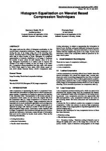
where 𝐼𝐽 and 𝐼𝐿 represent the mean intensity values of 𝐽 and 𝐿 in a local region Λ, respectively. 𝐴 and 𝑡 denote the mean values of airlight and scene transmission in Λ, respectively. Apparently, the remaining problem is how to fetch 𝑡 from a foggy image. Fortunately, dark channel prior makes it possible to get a rough 𝑡 that proceeds to be refined by soft-matting algorithm [9], as is shown in Figure 2. From the figure, the mean value of the rough 𝑡 in red or blue boxes is approximately close to that of the refined 𝑡. Accordingly, the mean rough 𝑡 may be adequate enough to equal 𝑡. Now that there is no need to calculate the refined 𝑡 that is the main cause for large time consumption in [9], it implies that we can obtain 𝑡 in patches promptly. Thus, when 𝐼𝐽 is substituted for
4
Mathematical Problems in Engineering The intensity component of a foggy image
The proposed variational framework Improvement for a mean brightness constraint
The estimation of airlight
Design for a spatial regularization term
A color attenuation prior
Pixel-based dark and bright channels
Design for a general variation filter
The intensity component of a fog-removal image
Figure 1: The flowchart of our proposed algorithm.
(a)
(b)
(c)
Figure 2: Comparison of mean local values in both rough and refined 𝑡 obtained by He et al. in [9]. In columns, a foggy image (a), rough 𝑡 (b), and refined 𝑡 (c). In rows, images in normal size and their zoom-in view of patches in red or blue frames.
𝜇(𝑥) in formula (6), a proper mean brightness constraint can be described as 2
1
∫ (∫ 𝑓ℎ𝑖 (𝑟, 𝑥) 𝑑𝑟 − 𝐼𝐽 (𝑥)) 𝑑𝑥 Ω
0
1
2
(1 − 𝑡) 1 = ∫ (∫ 𝑓ℎ𝑖 (𝑟, 𝑥) 𝑑𝑟 − 𝐼𝐿 (𝑥) + 𝐴) 𝑑𝑥, 𝑡 𝑡 0 Ω
(9)
when 𝑡 = 1, formula (9) turns to be ∫(∫ 𝑓ℎ𝑖 (𝑟, 𝑥)𝑑𝑟 − 𝐼𝐿 (𝑥))2 𝑑𝑥 which is only appropriate for regular image enhancement such as Iyad Jafar’s or Wei Wang’s works. Due to 0 < 𝑡 < 1 in foggy images, it is fully convinced that the modified constraint in formula (9) is more beneficial in foggy image restoration.
3.2. Design for a Spatial Regularization Term. First emerging in image restoration field, TV and 𝐻1 norms perform well and have their own merits. On the one hand, TV norm allows discontinuity of images and preserves more edges in textual regions, which is proven in [19]. On the other hand, [20] validates that 𝐻1 norm is able to keep the structural consistency in flat regions and costs fewer computer sources when the minimization of its regularization is processed. Given that we seek for a spatial regularization term that can imitate both of the two norms, to be specific, the expected regularization term should get close to TV norm in textual regions and behave like 𝐻1 norm in flat areas. Here, we suppose 𝜌(⋅) to be a function with respect to ∇𝑓 denoted by 𝑐 for the sake of clearness in the paper. If we have 𝜌(𝑐) = |𝑐|, then a TV norm is formed. In a similar
Mathematical Problems in Engineering
5 𝜌 (𝑐) 1 − 3𝑐2 𝑐→∞ → −3 ≤ 0 = 𝜌 (𝑐) /𝑐 1 + 𝑐2
way, a 𝐻1 norm is established when 𝜌(𝑐) = 𝑐2 . In order to imitate TV and 𝐻1 norms, it is reasonable to analyze the diffuse behavior of ∫ 𝜌(𝑐)𝑑𝑥 through its corresponding EulerLagrange equation: div [
𝜌 (|𝑐|) 𝑐] = 0. |𝑐|
(10)
𝜌 (|𝑐|) 𝜌 (|𝑐|) 𝑐] = 𝑓 div [ |𝑐| |𝑐| 𝜉𝜉
𝜌 (|𝑐|) 𝜌 (|𝑐|) +[ +( ) ⋅ |𝑐|] 𝑓𝜂𝜂 , |𝑐| |𝑐|
(11)
2 ∇𝑓 2 𝑑𝑥 𝑑𝑟. 1 + ∇𝑓
(16)
3.3. Construction and Calculation of the Proposed Framework. Combined with a mean brightness constraint in formula (9) and a spatial regularization term in formula (16), our variational framework of histogram equalization for image defogging is finally built up, which is depicted as 𝐸 (𝑓) = ∫
1 𝑓 (𝑟, 𝑥)2 𝑑𝑥 𝑑𝑟 ℎ𝑖 (𝑟, 𝑥) 𝑟 1
2
+ 𝛾1 ∫ (∫ 𝑓ℎ𝑖 (𝑟, 𝑥) 𝑑𝑟 − 𝐼𝐽 (𝑥)) 𝑑𝑥
𝑐→∞
(12)
𝜌 (𝑐) 𝑐→∞ → 𝜒 ≤ 0. 𝜌 (𝑐) /𝑐
𝜌 (𝑐) 𝑐→0 → 𝜅 𝑐
𝜌 (|𝑐|) 𝑐→0 ) → 0. ( |𝑐|
Λ
(13)
Based on those two rules of pointed diffuse behavior mentioned above, a satisfactory function is designed and turns out to be 𝑐2 . 1 + 𝑐2
(14)
It is easy to examine whether 𝜌(𝑐) obeys those two rules. Plugging 𝜌(𝑐) into formulas (12) and (13), we can get 𝜌 (𝑐) 𝑐→∞ 2 → 0 = 2 2 𝑐 (1 + 𝑐 ) 𝑐→∞
→ 0
Ω
+ 𝛾2 ∫
For another, if the speed in 𝜉 keeps as fast as that in direction 𝜂 in the flat regions, 𝜌(⋅) can be treated as 𝐻1 norm approximately. Therefore, the second rule is illustrated as
(1 +
Apparently, the function 𝜌(𝑐) is available. Thus, the spatial regularization term in formula (6) is changed into a new version:
Λ
𝜌 (𝑐) → 0
3 𝑐2 )
(15)
Λ
𝜌 (𝑐) 𝑐→∞ → 0 𝑐
2 − 6𝑐2
𝜌 (|𝑐|) 𝑐→0 −8𝑐 → 0. ) = 3 2 |𝑐| (1 + 𝑐 )
∫
where 𝑓𝜉𝜉 and 𝑓𝜂𝜂 represent tangential and normal components, respectively. Notice that it is available to control the diffuse speed of 𝑓𝜉𝜉 and 𝑓𝜂𝜂 . For one thing, if both of the speeds in tangential direction 𝜉 and normal direction 𝜂 gradually go to zero as 𝑐 grows up, together with the descending rate of speed in 𝜉 being lower than that in the other direction, it guarantees that 𝜌(⋅) is close to TV norm in the textural areas. Hence, the first rule can be listed as
𝜌 (𝑐) =
(
First of all, we would like to decompose the divergence term into two orthotropic components along the level set curve, as is shown in the following expression:
𝜌 (𝑐) =
𝜌 (𝑐) 𝑐→0 2 → 2 = 2 2 𝑐 (1 + 𝑐 )
0
(17)
2 ∇𝑓 2 𝑑𝑥 𝑑𝑟. 1 + ∇𝑓
From formula (17), our model is more concise in comparison with Wei Wang’s framework. The first term is utilized to enhance contrast through local histogram equalization while the second one aims at recovering the true brightness by enforcing the output brightness being close to 𝐼𝐽 (𝑥). The last one is devoted to preserving the structural consistency by minimizing the differences among local transformation functions. As to the solution of the proposed framework, we can learn from Wang’s algorithm. According to the alternating direction method of multipliers (ADMM) [21], formula (17) is converted into an unconstrained minimization problem through a pair of quadratic penalty functions. Thus, the whole process for minimizing 𝐸(𝑓) is actually a loop iteration containing two corresponding Euler-Lagrange equations. Relevant information about solving Euler-Lagrange equations can be found in [22, 23]. However, the time consumption is too expensive to be accepted. A possible way to accelerate the process is to deal with Euler-Lagrange equation through a TV filter [24]. Nevertheless, the regularization term |∇𝑓|2 /(1 + |∇𝑓|2 ) in our framework is not the same as TV norm |∇𝑓| exactly. If the fitted TV energy in the filter is replaced by a new energy, we have to adjust the filter coefficients, especially
6
Mathematical Problems in Engineering
the weights 𝑤𝛼𝛽 (𝑢). First of all, we might as well define the general form of a regularization term: 𝑅𝜌 (|∇𝑢|) = ∫ 𝜌 (|∇𝑢|) 𝑑Ω, Ω
(18)
where 𝜌(𝑐) is a monotone function. Then, it is easy to obtain the energy function’s Euler-Lagrange equation from an input image 𝑢0 in the discrete case [25]: 𝜕 −𝜌 (|∇𝑢|) 𝜕𝑢 ( ) + 𝜆 (𝑢𝛼0 − 𝑢𝛼 ) = 0, ∑ |∇𝑢| 𝜕ℓ 𝛼 𝛼∈ℓ 𝜕ℓ
(19)
where 𝛼 is one node of ℓ and (𝜕𝑢/𝜕ℓ)|𝛼 denotes the edge derivative. Focusing on the first term of formula (19), we proceed to define the discrete versions of |∇𝑢| and (𝜕𝑢/𝜕ℓ)|𝛼 as |∇𝑢| = √ ∑ ( 𝛼∈ℓ
2 𝜕𝑢 2 ) = √ ∑ (𝑢𝛽 − 𝑢𝛼 ) . 𝜕ℓ 𝛼 𝛼∈ℓ
(20)
With formula (20), we can get 𝜕 −𝜌 (|∇𝑢|) 𝜕𝑢 ( ) 𝜕ℓ |∇𝑢| 𝜕ℓ 𝛼 =(
−𝜌 (|∇𝑢|) 𝜕𝑢 −𝜌 (|∇𝑢|) 𝜕𝑢 ) − ( ) |∇𝑢| 𝜕ℓ 𝛽 |∇𝑢| 𝜕ℓ 𝛼
−𝜌 (∇𝛽 𝑢) 𝜕𝑢 𝜌 (∇𝛼 𝑢) 𝜕𝑢 ( = ) + ( 𝜕ℓ ) 𝜕ℓ 𝛽 ∇𝛽 𝑢 ∇𝛼 𝑢 𝛼 −𝜌 (∇𝛽 𝑢) 𝜌 (∇𝛼 𝑢) (𝑢 = − 𝑢 ) + (𝑢𝛽 − 𝑢𝛼 ) 𝛼 𝛽 ∇ 𝑢 ∇𝛼 𝑢 𝛽 𝜌 (∇𝛽 𝑢) 𝜌 (∇𝛼 𝑢) = ( ) (𝑢𝛽 − 𝑢𝛼 ) . + ∇𝛽 𝑢 ∇𝛼 𝑢
(21)
Now, it is available to describe the expression of 𝑤𝛼𝛽 (𝑢) from formula (22): 𝜌 (∇𝛽 𝑢) 𝜌 (∇𝛼 𝑢) . + ∇𝛽 𝑢 ∇𝛼 𝑢
2
2 2
(1 + ∇𝛽 𝑢 )
+
2
2 (1 + ∇𝛼 𝑢 )
(23)
Therefore, a general variation filter is formed to get a numerical solution from the energy functional framework precisely and promptly. In particular, 𝑤𝛼𝛽 (𝑢) goes to (1/|∇𝛼 𝑢| + 1/|∇𝛽 𝑢|) when 𝜌(𝑐) = 𝑐, which is brought into
2
.
(24)
3.4. The Estimation of Airlight. To recover the fog-free scene without yielding color shifting, the airlight is another important factor which is often neglected. It is simply inferred by selecting the brightest pixel of the entire image in [10]. Afterwards, He et al. pick up a pointed pixel that corresponds to the brightest one in the dark channel as the estimated airlight [9]. Then, Kim et al. merge quad-tree subdivision into a hierarchical searching strategy on purpose of obtaining a roughly inferred airlight [26]. Recently, people are devoted to seeking for an accurately estimated value. For example, Sulami et al. take a two-step estimating approach to recover the airlight through a geometric constraint and a global image prior [27]. Although they are remarkable in some situations, it is worth noting that these methods just provide a global constant airlight. Unfortunately, this is contrary to the fact that the airlight ought to vary with the fog density. Thus, we need to estimate a local airlight associated with the fog density. To recover the local airlight, the first step aims at measuring the fog density. We introduce a color attenuation prior [28] to measure the density for each pixel. The prior finds that the difference between the brightness and saturation is directly proportional to the depth. Moreover, it is well known that when the depth increases gradually, the fog density goes higher and higher. Based on these two observations, we can draw a conclusion about the relationship among the fog density 𝑞(𝑥), the depth 𝑑(𝑥), and the difference between the brightness V(𝑥) and the saturation 𝑠(𝑥): (25)
Because 𝐴(𝑥) varies along with the changes of 𝑞(𝑥), it is reasonable to make an assumption that 𝐴(𝑥) is positively proportional to 𝑞(𝑥) and we can get 𝐴 (𝑥) ∝ (V (𝑥) − 𝑠 (𝑥)) .
(22)
+ 𝜆 (𝑢𝛼0 − 𝑢𝛼 ) = 0.
𝑤𝛼𝛽 =
𝑤𝛼𝛽 =
𝑞 (𝑥) ∝ 𝑑 (𝑥) ∝ (V (𝑥) − 𝑠 (𝑥)) .
If formula (21) is plugged into formula (19), the discrete equation turns to be 𝜌 (∇𝛽 𝑢) 𝜌 (∇𝛼 𝑢) ∑ ( ) (𝑢𝛽 − 𝑢𝛼 ) + ∇𝛽 𝑢 ∇𝛼 𝑢 𝛼∈ℓ
correspondence with the weights of the TV filter. Now that 𝜌(𝑐) = 𝑐2 /(1 + 𝑐2 ) in our regularization term, the newly configured 𝑤𝛼𝛽 (𝑢) should be
(26)
Since there is one-to-one correspondence between 𝐴(𝑥) and 𝑞(𝑥), the maximum and minimum of 𝐴(𝑥) denoted by 𝐴+ (𝑥) and 𝐴− (𝑥) correspond to the highest and lowest fog density, respectively. Based on pixel-based dark channel 𝐽dark (𝑥) and pixel-based bright channel 𝐽bright (𝑥) [29], 𝐴+ (𝑥) and 𝐴− (𝑥) are simply defined as the pixels with the highest and lowest values in 𝐽dark (𝑥) and 𝐽bright (𝑥), respectively. 𝐽dark (𝑥) and 𝐽bright (𝑥) are mathematically expressed as 𝐽dark (𝑥) = min 𝐽𝑐 (𝑥) ,
(27)
𝐽bright (𝑥) = max 𝐽𝑐 (𝑥) .
(28)
𝑐∈{𝑅,𝐺,𝐵}
𝑐∈{𝑅,𝐺,𝐵}
Mathematical Problems in Engineering
7
Figure 3: Synthetic images named as L08005 and L08010: in the columns, foggy images and ground-truth images.
(a)
(b)
(c)
Figure 4: Results of our method initialized by different 𝛾1 : (a) 𝛾1 = 1, (b) 𝛾1 = 100, and (c) 𝛾1 = 10000.
AMBE index
0.06 0.05 0.04
0.0592 0.0464
0.0478 0.0357
0.0346
0.03
0.0238
0.02
0.0137
0.01 0
L08005 Parameter 𝛾1 1 10 100
0.0246 0.0144 0.005 L08010
1000 10000 (a)
MSE index
0.07
0.07 0.0618 0.0609 0.0571 0.0537 0.0557 0.0532 0.06 0.0489 0.0525 0.0466 0.05 0.0463 0.04 0.03 0.02 0.01 0 L08005 L08010 Parameter 𝛾1 1 10 100
1000 10000 (b)
Figure 5: Image quality of defogging results on L08005 and L08010 images is assessed by (a) AMBE index and (b) MSE index, respectively.
8
Mathematical Problems in Engineering
(a)
(b)
(c)
90 80 70 60 50 40 30 20 10 0
0.08
84.26
79.51
70.96
66.27
58.08
56.47 49.11
48.51
43.12
0.0758
0.07
41.59
MSE index
EI index
Figure 6: Results of our method initialized by different 𝛾2 : (a) 𝛾2 = 1, (b) 𝛾2 = 100, and (c) 𝛾2 = 10000.
0.06 0.0532 0.0514 0.0489 0.0488 0.05
0.0554
0.0608
0.0583 0.0558 0.0557
0.04 0.03 0.02 0.01 0
L08005 Parameter 𝛾2 1 10 100
L08010
L08005 Parameter 𝛾2 1 10 100
1000 10000 (a)
L08010
1000 10000 (b)
Figure 7: Image quality of defogging results on L08005 and L08010 images is assessed by (a) EI index and (b) MSE index, respectively.
According to formula (26) with two known points: (max(V(𝑥) − 𝑠(𝑥)), 𝐴+ (𝑥)) and (min(V(𝑥) − 𝑠(𝑥)), 𝐴− (𝑥)), a local 𝐴(𝑥) can be estimated by 𝐴 (𝑥) =
𝐴+ (𝑥) − 𝐴− (𝑥) (V (𝑥) − 𝑠 (𝑥)) 𝜃+ (𝑥) − 𝜃− (𝑥) 𝐴− (𝑥) ⋅ 𝜃+ (𝑥) − 𝐴+ (𝑥) ⋅ 𝜃− (𝑥) , + 𝜃+ (𝑥) − 𝜃− (𝑥)
can infer 𝐼𝐽 from the variational framework and then 𝑆𝐽 is obtained by formula (5). At last, 𝐽(𝑥) can be easily recovered with 𝐼𝐽 and 𝑆𝐽 .
4. Experiments and Analysis (29)
where max(V(𝑥) − 𝑠(𝑥)) and min(V(𝑥) − 𝑠(𝑥)) denoted by 𝜃+ (𝑥) and 𝜃− (𝑥) are constants. With the estimated 𝐴(𝑥), we
In order to perform a qualitative and quantitative analysis of the proposed method, we do some simulation experiments on color foggy images in comparison with three pairs of state-of-the-art defogging approaches. The first pair is Ranota and Kaur’s [13] and Wang and Ng’s [14] that are directly
Mathematical Problems in Engineering
(a)
9
(b)
(c)
Figure 8: Comparison of results on house image obtained by Ranota’s method, Wang’s method, and ours. In the columns, an original foggy image, fog-removal results processed by Ranota’s method (up), Wang’s method (middle), and ours (down), corresponding zoom-in view of red or blue boxes.
based on histogram equalization technique while the second one is Arigela and Asari’s [11] and Liu et al.’s [12] which belong to intensity transformation functions. Apparently, it is indispensable for us to choose them as comparative groups, since they are quite relevant to our method. He et al.’s [9] and Nishino et al.’s [10] in the last pair are classical and representative, as is well known in the image defogging field. Thus, we are going to compare our method with all of them pair by pair on the foggy image set that contains benchmarked and realistic images chosen from [9–14]. 4.1. Test of Parameters. Before the comparison, we ought to inform the experimental condition and the parameter selection. All the mentioned approaches are carried out in the MATLAB R2014a environment on a 3.5 GHz computer with 4 GB RAM. On the simulation platform, the parameters utilized in our method are set to be 𝜆01 = 𝜆02 = 𝜆03 = 0, 𝛽 = 1,
𝛾1 = 100, and 𝛾2 = 100. It is worth pointing out that 𝛾1 and 𝛾2 are picked up from several pairs of (𝛾1 , 𝛾2 ), where 𝛾1 , 𝛾2 ∈ {1, 10, 100, 1000, 10000} in the parameter-testing experiment. Specifically, two synthetic images are chosen from Frida database, as shown in Figure 3. Besides, three assessment indexes are introduced to evaluate the effectiveness of our method initialized by different pairs of (𝛾1 , 𝛾2 ). The first index is the absolute mean brightness error (AMBE) that is the difference of mean brightness between the output and the ground-truth image while the second one is edge intensity (EI) which quantifies the structural information. The last one is the mean square error (MSE) that measures the change of the output in comparison with the ground-truth image. Notice that AMBE index and MSE index belong to backward pointers. Their scores range from 0 to 1, and the lower they are, the better image quality will be. EI index is on the opposite side where higher scores imply better results.
10
Mathematical Problems in Engineering
(a)
(b)
(c)
Figure 9: Comparison of results on trees image obtained by Ranota’s method, Wang’s method, and ours. In the columns, an original foggy image, fog-removal results processed by Ranota’s method (up), Wang’s method (middle), and ours (down), corresponding zoom-in view of red or blue boxes.
Firstly, we might as well fix 𝛾2 on 100 and adjust 𝛾1 freely. Figure 4 describes a part of results processed with different 𝛾1 and Figure 5 is the quantitative evaluation of performance by AMBE and MSE indexes. From Figure 5(a), AMBE index is decreasing along with the increasing 𝛾1 , due to the fact that 𝛾1 is directly related to the second term in formula (17). It means that the higher 𝛾1 is, the better the mean brightness of results will be. However, it can be seen from Figure 5(b) that MSE index keeps decreasing at a slow speed after 𝛾1 reaches 100, which implies that merely resorting to increasing 𝛾1 is not enough to remove the fog degradation. Worse still, a higher 𝛾1 is prone to induce more iterations in the solution-calculating step. Therefore, it is logical to set 𝛾1 to be 100 in the proposed framework. Secondly, 𝛾1 is fixed on 100 and 𝛾2 can be adjusted from 1 to 10000. Processed results of our method initialized by different 𝛾2 are presented partially and evaluated, as shown in Figures 6 and 7, respectively. At first sight of Figure 6, results suffer from a great loss of contrast when 𝛾2 increases gradually. This observation is strengthened by Figure 7(a) where EI index, as a measurement of image contrast, becomes smaller and smaller. Nevertheless, it does not mean that the higher 𝛾2 is, the worse image quality will be. From Figure 6, the structural consistency keeps better along with the increasing 𝛾2 . This is because 𝛾2 affects both of image contrast and structural consistency, according to the first and third terms in formula (17). The contradictory relationship between the
contrast and consistency is validated by Figure 7(b) where MSE index is in the shape of “U” with high at two ends and low in middle, given that it is a compromise that 𝛾2 is set to be 100 in the proposed method. 4.2. Qualitative Comparison 4.2.1. Qualitative Comparison with Histogram-EqualizationBased Methods. Since our method is based on a variational histogram equalization framework, it is acceptable to be compared with Ranota and Kaur’s [13] and Wang and Ng’s [14] on house and trees images. From Figures 8 and 9, results obtained by Ranota’s method are in artificial color and dark patches. In contrast, results processed by Wang’s method and ours are quite superior in terms of color fidelity and local structure. The reasons can be summed up into two aspects: for one thing, Wang’s method and ours avoid distorted color by treating 𝐼 and 𝑆 components differently, unlike Ranota’s processing all of color components in the same way; for another, Gaussian filter in Ranota’s method tends to smoothen the rough scene transmission as well as local contrast at the same time. Wang’s method and ours which do not need to refine the scene transmission will not produce the structural distortion. However, in comparison with our results, Wang’s method seems to be brighter in the global illumination. For example, the grasses in blue box of Figure 8(c) are too bright to exhibit their real color
Mathematical Problems in Engineering
(a)
11
(b)
(c)
Figure 10: Comparison of results on street image obtained by Arigela’s method, Liu’s method, and ours. In the columns, an original foggy image, fog-removal results processed by Arigela’s method (up), Liu’s method (middle), and ours (down), corresponding zoom-in view of red or blue boxes.
information, so is the road in blue box of Figure 9(c). This is largely because Wang’s method preserves the mean brightness of an input foggy image. Thanks to the revised brightness constraint in our framework, the color is recovered properly. Moreover, from the results of Wang’s method based on TV norm in the house image and 𝐻1 norm in the trees image,
the structural consistency between the wall and the branch is violated in the middle red box of Figure 8(c). What is worse, many details of branches are lost in the middle red box of Figure 9(c). The main reason is that TV and 𝐻1 norms are unable to preserve the consistency and fine details in the discontinuity of textural regions simultaneously. With the
12
Mathematical Problems in Engineering
(a)
(b)
(c)
Figure 11: Comparison of results on train image obtained by Arigela’s method, Liu’s method, and ours. In the columns, an original foggy image, fog-removal results processed by Arigela’s method (up), Liu’s method (middle), and ours (down), corresponding zoom-in view of red or blue boxes.
help of a designed regularization term in our method, there is no need to sacrifice the consistency for fine details and vice versa. 4.2.2. Qualitative Comparison with Intensity-TransformationBased Methods. Histogram equalization and intensitytransformation-based methods are similar enhancement algorithms, so we launch a comparison among Arigela’s method [11], Liu et al.’s method [12], and ours on street and train images. As exhibited in Figure 10 (up) and Figure 11 (up), Arigela’s results are still in dim color with the sky and white objects being accompanied with halo effect. This is because Arigela’s method substitutes intensity transformation function for soft-matting algorithm used in He’s method [9] so as to refine a rough scene transmission. It means that the method is in close relationship with He’s and therefore its results inevitably suffer from the same unwanted distortion as He’s does exactly. A further explanation will be found in Section 4.2.3. Liu’s method does not seek for an accurate scene transmission and its results are displayed in Figure 10 (middle) and Figure 11 (middle). They show fine local details and abundant color information, because the method
removes fog degradation with intensity transformation function guided by scene depth layers. Nevertheless, Liu’s results present an oversaturation appearance, due to a lack of color fidelity constraint. Compared with those two defogging methods, ours can produce pleasing results with vivid color and great contrast. The success may owe to the constrained variational framework with a color fidelity term. 4.2.3. Qualitative Comparison with Classical and Representative Methods. To make the performance of the proposed method more persuasive and convincing, it is a must to compare our method with several classical and representative ones such as He et al.’s [9] and Nishino et al.’s [10]. From Figures 12 and 13, results delivered by He’s and Nishino’s method are recovered up to a reasonable level, so does the proposed method. However, the scene color of He’s and Nishino’s results should have been bright, but stay quite dim instead. For instance, the color of grasses on the rocks is nearly concealed so that we could not tell the difference between grasses and rocks in the blue box of Figure 12 (up) and Figure 12 (middle), so is the one of buildings in the blue box of Figure 13 (up) and Figure 13 (middle). The
Mathematical Problems in Engineering
(a)
13
(b)
(c)
Figure 12: Comparison of results on cliff image obtained by He’s method, Nishino’s method, and ours. In the columns, an original foggy image, fog-removal results processed by He’s method (up), Nishino’s method (middle), and ours (down), corresponding zoom-in view of red or blue boxes.
reason that He’s method induces over-defogging results is mainly due to dark channel prior that overestimates the thickness of fog. The predicted transmission value is lower or much lower sometimes than the true one when it is filtered by “min” filters, which has been pointed out in [30]. The reason for Nishino’s method is the same thing, since statistical distributions are considered as depth prior absorbed in the probabilistic minimization. Worse still, false color and blocking artifacts occur in the regions of He’s and Nishino’s results, as is shown in the red boxes of Figures 12 and 13. It is due to the different ways of their estimating the airlight. Both of them consider the roughly estimated airlight to be a global constant, which goes against the basic fact that the airlight varies with the fog density. Different from their methods, the proposed one estimates a local airlight associated with the fog density under a color attenuation prior and pixel-based bright and dark channels. Apparently, our method has the capability of removing fog effects without yielding unappealing distortion or information loss.
4.3. Quantitative Comparison. In order to strengthen the qualitative analyses mentioned above, two no-reference assessment indexes are introduced, including EI index and no-reference image quality evaluator index (NIQE) [31]. It is worth noting that among those three indexes in Section 4.1, AMBE index and MSE index are full-reference evaluators. They are inappropriate for assessing image quality with the absence of ground-truth images. Accordingly, only EI index is adopted to evaluate the structural contrast again in this section. Plus, NIQE index is meant to measure the distortion degree of processed results through scene statistics of locally normalized luminance coefficients. Actually, the shape of those coefficients’ distribution in a foggy image is thinner than the one in a defogged image, which implies NIQE index is capable of quantifying the losses of naturalness from a distorted image. Scores of the index distribute from 0 to 100 and zero score represents the best result. Figures 14–16 give a series of quantitative assessments for images in Figures 8–13. As displayed in the plots of Figures 14–16, results processed by
14
Mathematical Problems in Engineering
(a)
(b)
(c)
Figure 13: Comparison of results on tower image obtained by He’s method, Nishino’s method, and ours. In the columns, an original foggy image, fog-removal results processed by He’s method (up), Nishino’s method (middle), and ours (down), corresponding zoom-in view of red or blue boxes.
our method gain the best scores of EI index and NIQE index. This fully shows that the proposed method can produce more plausible results, compared with the other algorithms. The time consumption needs to be taken into consideration, if the method is put into the practice. Figure 17 exhibits the running time of several defogging methods previously mentioned. From the figure, He’s and Nishino’s methods cost the most time sources above all. This is because they depend much on the accurate scene transmission refined by the softmatting algorithm or a jointly estimated Bayesian framework that takes up plenty of time. Except for He’s and Nishino’s methods, Wang’s method also consumes too much time up to 15 seconds which is three times as much as the cost of the remaining four methods. The reason is that two EulerLagrange equations are required to be tacked in every loop iteration. Compared with Wang’s work, our method proposes a general variation filter to solve the Euler-Lagrange equation, resulting in saving considerable time. Moreover, the time cost of Ranota’s, Arigela’s, and Liu’s methods also keep at a comfortably lower level, since they are based on image enhancement algorithms.
5. Conclusion In the paper, we propose an image defogging method using a variational histogram equalization framework. A previous variational framework on image enhancement inspires us to establish a constrained energy functional that contains histogram equalization and the physical degradation model. The mean brightness constraint in the framework is revised to preserve the brightness of a fog-free image while the regularization term is redesigned for avoiding manual intervention. To pursue the processing efficiency, a general variation filter is proposed to solve the constrained framework promptly. As to another important unknown quantity 𝐴, a color attenuation prior and pixel-based dark and bright channels are introduced to infer a local constant 𝐴 reasonably. In the end, the proposed method is tested on several benchmarked and realistic images in comparison with three groups of representative defogging methods. With qualitative and quantitative comparison, it is safe to draw a conclusion that our method performs much better in terms of color adjustment and contrast enhancement. In the future, more
180 160 140 120 100 80 60 40 20 0
15
149.4683 157.8979 111.6164 118.4214 88.5126
NIQE index
EI index
Mathematical Problems in Engineering
104.1377
House
16 14 12 10 8 6 4 2 0
13.8762
4.6015
2.6572
House
Trees
Defogging methods Ranota’s method Ours
7.3215
5.7666
Trees
Defogging methods Ranota’s method Ours
Wang’s method
1.8697
Wang’s method
(a)
(b)
140 120 100 80 60 40 20 0
12 116.9585 68.5053
10 50.6521 66.2798 44.1146
28.9408
NIQE index
EI index
Figure 14: Image quality of defogging results on house and trees images obtained by Ranota’s method, Wang’s method, and ours is assessed by (a) EI index and (b) NIQE index.
9.8976
10.064
9.2862
7.0718
8 6
4.8749 3.3501
4 2
Street Defogging methods Arigela’s method Ours
0
Train
Street Defogging methods Arigela’s method Ours
Liu’s method (a)
Train
Liu’s method (b)
70 60 50 40 30 20 10 0
12
59.876 33.8662 22.7732
20.2303
18.7254
10.9864 10.4285
10
51.1282 NIQE index
EI index
Figure 15: Image quality of defogging results on street and train images obtained by Arigela’s method, Liu’s method, and ours is assessed by (a) EI index and (b) NIQE index.
8 6
4.6891
4.3344 3.6494
4
2.7977
2 Cliff Defogging methods He’s method Ours
Tower
Nishino’s method (a)
0 Cliff Defogging methods He’s method Ours
Tower
Nishino’s method (b)
Figure 16: Image quality of defogging results on cliff and tower images obtained by He’s method, Nishino’s method, and ours is assessed by (a) EI index and (b) NIQE index.
Mathematical Problems in Engineering 18 16 14 12 10 8 6 4 2 0
6
15.36 13.47
5
4.27
3.71
Time cost (s)
Time cost (s)
16
4.63
3.99
5.38
5.05
4.47
4.09
4
2.96
3
2.73
2 1 0
House Defogging methods Ranota’s method Ours
Street
Trees
Train
Defogging methods Arigela’s method Ours
Wang’s method
Liu’s method (b)
Time cost (s)
(a)
40 35 30 25 20 15 10 5 0
35.15
32.21 21.69
23.42
6.03
5.24 Cliff Defogging methods He’s method Ours
Tower
Nishino’s method (c)
Figure 17: Time consumption for three groups of defogging methods including Ranota’s method, Wang’s method, Arigela’s method, Liu’s method, He’s method, Nishino’s method, and ours.
attention will be put on accelerating the processing speed up to a real-time level for some computer vision applications.
Competing Interests The authors declare that they have no competing interests.
References [1] N. Hauti`ere, J.-P. Tarel, H. Halmaoui, R. Br´emond, and D. Aubert, “Enhanced fog detection and free-space segmentation for car navigation,” Machine Vision and Applications, vol. 25, no. 3, pp. 667–679, 2014. [2] H. Liu, J. Yang, Z. Wu, and Q. Zhang, “Fast single image dehazing based on image fusion,” Journal of Electronic Imaging, vol. 24, no. 1, Article ID 013020, 2015. [3] J.-G. Wang, S.-C. Tai, and C.-J. Lin, “Image haze removal using a hybrid of fuzzy inference system and weighted estimation,” Journal of Electronic Imaging, vol. 24, no. 3, Article ID 033027, pp. 1–14, 2015. [4] N. S. Narasimhan and S. Nayar, “Interactive (de) weathering of an image using physical models,” in Proceedings of the IEEE Workshop on Color and Photometric Methods in Computer Vision, pp. 1–8, October 2003. [5] Y. Y. Schechner, S. G. Narasimhan, and S. K. Nayar, “Instant dehazing of images using polarization,” in Proceedings of the
2001 IEEE Computer Society Conference on Computer Vision and Pattern Recognition, pp. I325–I332, December 2001. [6] S. G. Narasimhan and S. K. Nayar, “Vision and the atmosphere,” International Journal of Computer Vision, vol. 48, no. 3, pp. 233– 254, 2002. [7] Y. Lee, K. B. Gibson, Z. Lee, and T. Q. Nguyen, “Stereo image defogging,” in Proceedings of the IEEE International Conference on Image Processing (ICIP ’14), pp. 5427–5431, Paris, France, October 2014. [8] J. Kopf, B. Neubert, B. Chen et al., “Deep photo: Model-based photograph enhancement and viewing,” ACM Transactions on Graphics, vol. 27, no. 5, article 116, 2008. [9] K.-M. He, J. Sun, and X.-O. Tang, “Single image haze removal using dark channel prior,” IEEE Transactions on Pattern Analysis and Machine Intelligence, vol. 33, no. 12, pp. 2341–2353, 2010. [10] K. Nishino, L. Kratz, and S. Lombardi, “Bayesian defogging,” International Journal of Computer Vision, vol. 98, no. 3, pp. 263– 278, 2012. [11] S. Arigela and V. K. Asari, “Enhancement of hazy color images using a self-tunable transformation function,” in Advances in Visual Computing, G. Bebis, R. Boyle, B. Parvin et al., Eds., vol. 8888 of Lecture Notes in Computer Science, pp. 578–587, Springer, New York, NY, USA, 2014. [12] Q. Liu, M. Y. Chen, and D. H. Zhou, “Single image haze removal via depth-based contrast stretching transform,” Science China Information Sciences, vol. 58, no. 1, pp. 1–17, 2015.
Mathematical Problems in Engineering [13] H. K. Ranota and P. Kaur, “A new single image dehazing approach using modified dark channel prior,” Advances in Intelligent Systems and Computing, vol. 320, pp. 77–85, 2015. [14] W. Wang and M. K. Ng, “A variational histogram equalization method for image contrast enhancement,” SIAM Journal on Imaging Sciences, vol. 6, no. 3, pp. 1823–1849, 2013. [15] R. C. Gonzalez and R. E. Woods, Digital Image Processing, Publishing House of Electronics Industry, Beijing, China, 3rd edition, 2010. [16] I. Jafar and H. Ying, “Image contrast enhancement by constrained variational histogram equalization,” in Proceedings of the IEEE International Conference on Electro/Information Technology (EIT ’07), pp. 120–125, Chicago, Ill, USA, May 2007. [17] R. Fattal, “Single image dehazing,” ACM Transactions on Graphics, vol. 27, no. 3, article 72, 2008. [18] R. T. Tan, “Visibility in bad weather from a single image,” in Proceedings of the 26th IEEE Conference on Computer Vision and Pattern Recognition (CVPR ’08), pp. 1–8, Anchorage, Alaska, USA, June 2008. [19] L. I. Rudin, S. Osher, and E. Fatemi, “Nonlinear total variation based noise removal algorithms,” Physica D. Nonlinear Phenomena, vol. 60, no. 1–4, pp. 259–268, 1992. [20] G. Aubert and P. Kornprobst, Mathematical Problems in Image Processing: Partial Differential Equations and the Calculus of Variations, vol. 147, Springer, New York, NY, USA, 2002. [21] F. Lin, M. Fardad, and M. R. Jovanovic, “Design of optimal sparse feedback gains via the alternating direction method of multipliers,” IEEE Transactions on Automatic Control, vol. 58, no. 9, pp. 2426–2431, 2013. [22] C. R. Vogel and M. E. Oman, “Fast, robust total variation-based reconstruction of noisy, blurred images,” IEEE Transactions on Image Processing, vol. 7, no. 6, pp. 813–824, 1998. [23] A. Marquina and S. Osher, “Explicit algorithms for a new time dependent model based on level set motion for nonlinear deblurring and noise removal,” SIAM Journal on Scientific Computing, vol. 22, no. 2, pp. 387–405, 2000. [24] T. F. Chan, S. Osher, and J. Shen, “The digital TV filter and nonlinear denoising,” IEEE Transactions on Image Processing, vol. 10, no. 2, pp. 231–241, 2001. [25] G. Aubert and L. Vese, “A variational method in image recovery,” SIAM Journal on Numerical Analysis, vol. 34, no. 5, pp. 1948–1979, 1997. [26] J.-H. Kim, J.-Y. Sim, and C.-S. Kim, “Single image dehazing based on contrast enhancement,” in Proceedings of the 36th IEEE International Conference on Acoustics, Speech, and Signal Processing (ICASSP ’11), pp. 1273–1276, Prague, Czech Republic, May 2011. [27] M. Sulami, I. Glatzer, R. Fattal, and M. Werman, “Automatic recovery of the atmospheric light in hazy images,” in Proceedings of the 6th IEEE International Conference on Computational Photography (ICCP ’14), pp. 1–11, May 2014. [28] Q. Zhu, J. Mai, and L. Shao, “A fast single image haze removal algorithm using color attenuation prior,” IEEE Transactions on Image Processing, vol. 24, no. 11, pp. 3522–3533, 2015. [29] C.-H. Yeh, L.-W. Kang, C.-Y. Lin, and C.-Y. Lin, “Efficient image/video dehazing through haze density analysis based on pixel-based dark channel prior,” in Proceedings of the 3rd International Conference on Information Security and Intelligent Control (ISIC ’12), pp. 238–241, Yunlin, Taiwan, August 2012. [30] K. Tang, J. Yang, and J. Wang, “Investigating haze-relevant features in a learning framework for image dehazing,” in
17 Proceedings of the 27th IEEE Conference on Computer Vision and Pattern Recognition (CVPR ’14), pp. 2995–3002, Columbus, Ohio, USA, June 2014. [31] A. Mittal, A. K. Moorthy, and A. Bovik, “No-reference image quality assessment in the spatial domain,” IEEE Transactions on Image Processing, vol. 21, no. 12, pp. 4695–4708, 2012.
Advances in
Operations Research Hindawi Publishing Corporation http://www.hindawi.com
Volume 2014
Advances in
Decision Sciences Hindawi Publishing Corporation http://www.hindawi.com
Volume 2014
Journal of
Applied Mathematics
Algebra
Hindawi Publishing Corporation http://www.hindawi.com
Hindawi Publishing Corporation http://www.hindawi.com
Volume 2014
Journal of
Probability and Statistics Volume 2014
The Scientific World Journal Hindawi Publishing Corporation http://www.hindawi.com
Hindawi Publishing Corporation http://www.hindawi.com
Volume 2014
International Journal of
Differential Equations Hindawi Publishing Corporation http://www.hindawi.com
Volume 2014
Volume 2014
Submit your manuscripts at http://www.hindawi.com International Journal of
Advances in
Combinatorics Hindawi Publishing Corporation http://www.hindawi.com
Mathematical Physics Hindawi Publishing Corporation http://www.hindawi.com
Volume 2014
Journal of
Complex Analysis Hindawi Publishing Corporation http://www.hindawi.com
Volume 2014
International Journal of Mathematics and Mathematical Sciences
Mathematical Problems in Engineering
Journal of
Mathematics Hindawi Publishing Corporation http://www.hindawi.com
Volume 2014
Hindawi Publishing Corporation http://www.hindawi.com
Volume 2014
Volume 2014
Hindawi Publishing Corporation http://www.hindawi.com
Volume 2014
Discrete Mathematics
Journal of
Volume 2014
Hindawi Publishing Corporation http://www.hindawi.com
Discrete Dynamics in Nature and Society
Journal of
Function Spaces Hindawi Publishing Corporation http://www.hindawi.com
Abstract and Applied Analysis
Volume 2014
Hindawi Publishing Corporation http://www.hindawi.com
Volume 2014
Hindawi Publishing Corporation http://www.hindawi.com
Volume 2014
International Journal of
Journal of
Stochastic Analysis
Optimization
Hindawi Publishing Corporation http://www.hindawi.com
Hindawi Publishing Corporation http://www.hindawi.com
Volume 2014
Volume 2014