Color Image Segmentation using MRF and ... - Semantic Scholar

Proceedings of Soft Computing Technique for Engineering applications SCT-2006, Rourkela March 24-26,2006. Archived in Dspace@NITR http://dspace.nitrkl.ac.in/dspace

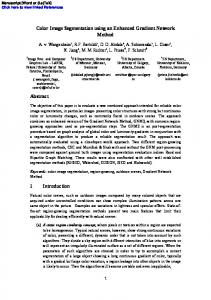
Color Image Segmentation Using MRF Model and Simulated Annealing #P.J. Mohapatra, P. K. Nanda and S. Panda Image Processing and Computer Vision Lab. Department of Electrical Engineering National Institute of Technology, Rourkela 769008 [email protected], [email protected], [email protected] Abstract In this paper color image segmentation is accomplished using MRF model. The problem is formulated as a pixel labeling and the true labels are modeled as the MRF model. The observed color image is assumed to be the degraded version of the true labels. We assume the degradation to be Gaussian distribution. The label estimates are obtained by using Bayesian framework and MAP criterion. The (I1, I2, I3) color model is used to represent the color and the MAP estimate is obtained by Simulated Annealing. Simulation results of both indoor and outdoor scenes are considered to validate our approach. Index Terms

(I1, I2, I3) color Space, MAP Estimate, Segmentation, Simulated Annealing (SA)

1

Introduction Image segmentation is an important issue in several applications of image processing

and computer vision. It is the process of partitioning an image into disjoint and homogeneous regions [1], [2]. A homogeneous region refers to a group of connected pixels in an image which share a common feature. This feature could be color, texture, brightness, motion etc. A common problem of segmenting a monochrome image occurs when an image has a background of varying gray level such as gradually changing shades. Compared to a monochrome image, a color image provides additional information on the objects in the image. Color information provides more complete representation of image and more reliable segmentation can be achieved as compared to only gray level image. Earlier processing of color images require a very high computation time. But now-a-days this problem can be avoided with increasing speed and decreasing cost of computation. In many object recognition or tracking applications color

segmentation plays a major role where color provides a distinguishing feature of the object of interest. Recent research focuses on color image segmentation due to its growing need [1]. Often MRF is used as the image model for color image segmentation. Basically, neighborhood based approaches use both intensity information and the spatial knowledge. This means that the labels of a pixel depends not only its color but also in its neighbor’s color. So, these approaches are more robust with respect to noise than histogram based approaches. Dileep Panjwani et al [4] proposed a selection of random filed models for color images. Models are defined in terms of set of neighbors which characterize interaction within and between three bands of a color image [5]. An unsupervised color image segmentation algorithm is presented using an MRF pixel classification model [6] and J. Mukherjee[7] proposed a segmentation algorithm based on MRF processing. An MRF approach of color image segmentation enhanced by edge detection is presented in [8],[9]. Huawu Deng et al [10] proposed a model for unsupervised segmentation of gray level as well as color images. In this paper, we have presented a color image segmentation algorithm which uses Markov Random Field (MRF) model. The problem is formulated as a pixel labeling problem. True labels of the color image are modeled as the MRF model. Bayesian image segmentation is achieved with the help of maximum a posteriori (MAP) estimation combining with MRF model [3]. The (I1, I2, I3) color space is used to represent the color image. We have proposed a supervised classification to perform color image segmentation. Pixel classes are represented by multivariate Gaussian distributions and a first order MRF model is used. SA algorithm is used to obtain the MAP estimate.

2

Color Model A color image can be represented by its Red (R), Green (G) and Blue (B) spectral

components. These components are transformed to other color spaces depending upon the problem being considered. The image defined in RGB space can be converted into other color spaces either by linear transformation or nonlinear transformation. The choice of a color model has a significant effect on the segmentation result. Hence, there are two critical issues for color

image segmentation (i) What segmentation method should be utilized and (ii) Which color space should be used in order to obtain a better segmentation result. In this paper, we have adopted I1I2I3 (Ohta’s) color space. This color space is used for segmentation due to the following reasons [1]: (a) It is more effective in terms of quality of segmentation. (b) Also, in terms of computational complexity of the transformation. The transformation used to obtain I1I2I3 from RGB color space is given below. ⎡ I1 ⎢ ⎢I2 ⎢I ⎣ 3

3

⎤ ⎡ 13 ⎥ ⎢1 ⎥ = ⎢ 2 ⎥ ⎢− 1 4 ⎦ ⎣

1

3

1

3 − 12 1 1 2 − 4 0

⎤⎡R ⎥⎢ ⎥ ⎢G ⎥⎢B ⎦⎣

⎤ ⎥ ⎥ ⎥⎦

(1)

MRF Model We assumed all the images to be defined on a discrete rectangular lattice M = (N x N).

Let Z denote the label process associated with the given noise free image X and z be a realization of Z. We model the label process Z of the image as MRF. The observed image X is assumed to be a random field that is the sum of the label process Z and the corruptive noise random field W. The noise free label process Z is assumed to be a Markov random field with respect to a neighborhood system η, and is described by in terms of its local characteristics. P ( Z i , j = z i , j | Z k , l = z k , l , k , l ∈ N × N , ( k , l ) ≠ ( i , j ))

(2)

= P ( Z i , j = z i , j | Z k ,l = z k ,l , ( k , l ) ∈ η )

Here Z is an MRF or equivalently Gibb’s distributed (GD) which is considered as a priori distribution. This is expressed as P ( Z = z |φ ) =

1 Z

'

e

−U ( z ,φ ) where Z ' = ∑ e −U ( z ,φ ) is the

z

partition function, φ represents the clique parameter vector, the exponent term U ( Z , φ ) is called the energy function and is of the form U ( Z , φ ) =

V c ( z , φ ) , where Vc ( z , φ ) ∑ C: (i , j )∈c

being referred to as the potential. The image model considered is X i , j = Z i , j + Wi , j ,

∀ (i , j ) ∈ ( N x N )

(3)

Which with a lexicographical ordering will be Y = Z + W. We make the following assumptions: (a) Wi, j is a white Gaussian sequence with zero mean variance σ2. (b) Wi,

j

is

statistically independent of Zk, l , for all (i, j) and (k, l) belonging to N x N. (c) zi, j takes any value from the label set M = (1, 2, .................., M m ), (typically Mm= 256). Note, in general the unknown parameter vector θ = [ φ

4

T

,σ

2

].

Problem Formulation Let X be the observed color image which is considered as a realization of a random

field. The problem is to find the true label of X, hidden in it. The segmentation problem can be formulated as finding the true label of the given observed image X. Let us suppose that the observed image X = { x s | s ε S } consists of three spectral component values at each pixel s є S denoted by the vector xs. Let Z be the segmented image which represents the true label process, which is assumed to be an MRF. Let z є Z is a realization of the label process and x є X is a realization of the observed process. The labeling

zˆ is obtained by maximizing the posteriori probability P ( Z = z | X = x, θ ) . Hence, the optimality criterion is zˆ = arg max P ( Z = z | X = x, θ ) z

(4)

Since z is unknown the above can not be computed. So, by using Baye’s theorem [3], hence (4) can be expressed as P ( X = x | Z = z,θ )P (Z = z)

zˆ = arg max z

(5)

P ( X = x |θ )

Since X corresponds to the given image P ( X = x | θ ) is constant. P ( Z = z ) is the a priori probability of the labels. According to Hammersley-Clifford theorem P(Z = z) =

1 Z

'

e

−U ( z ) T

(6)

Where, Z’ = normalizing constant or partition function and T = Temperature which controls the sharpness of the distribution. Usually T is taken as 1.

The only unknown remaining in (5) is the P ( X = x | Z = z , θ ) . Here we assume that the observed image can be considered as a transformed and degraded version of an MRF realization. Using the degradation image model of (3), P ( X = x | Z = z , θ ) can be written as P( X = x | Z = z,θ ) = P( X = z + w | Z ,θ )

(7)

= P (W = x − z | Z , θ )

Since W is a Gaussian process and using the assumption stated in section 3 we obtain P (W = x − z | Z , θ ) =

( 2π )

1 n

− 1 ( x − z )T K −1 ( x − z ) e 2

(8)

det[ K ]

Where K is the covariance matrix. Since we are considering three independent components of the color such as I1, I2, and I3, the noise distribution is a multivariate one. Equation (8) reduces to P (W = x − z | Z , θ ) =

−

1 ( 2π )

3

σ

3

e

1 ( x − z )2 2σ 2

(9)

Substituting (9) and (6) in (5) we have ⎤ ( x − z )2 + U ( z ) ⎥⎥ 2 ⎢⎣ 2σ ⎥⎦ ⎡

1 P ( Z = z | X = x , θ ) = arg max e ' 3 3 z Z ( 2π ) σ

− ⎢⎢

(10)

The maximization of the above function is equal to the minimization of the following.

⎡ (x − z) 2

zˆ = arg min ⎢ z ⎢⎣

2σ

2

⎤

(11)

+ U ( z )⎥

⎥⎦

For color image (11) can be represented as

⎡ ( x1 − z1 ) 2 + ( x 2 − z 2 ) 2 + ( x 3 − z 3 ) 2

zˆ = arg min ⎢ z ⎣⎢

2σ

2

1 2 3 ⎤ + ∑ Vc ( z , z , z )⎥ c∈ C ⎥

(12)

⎦

where Vc is the clique potential function for all the three components, C is the set of all cliques and 1,2 and 3 indicate the three spectral components.

5

Simulated Annealing Algorithm Simulated Annealing (SA) algorithm has been proposed by Kirkpatrick [11], [12]. The

Simulated Annealing (SA) is used to obtain the MAP estimate. The SA process consists of melting the system being optimized at a high effective temperature, then lowering the temperature by slow stages until the system freezes and no further changes occur. SA extends to one of the most widely used heuristic techniques. Large changes in the objective function occur at high temperature while the small changes are deferred until low temperatures. The steps of the SA algorithm are described below [11],[12]. 1.

Initialize the temperature Tin.

2.

Compute the energy U of the configuration.

3.

Perturb the system slightly with suitable Gaussian disturbance.

4.

Compute the new energy U’ of the perturbed system and evaluate the change in the energy ∆U = U – U’.

5.

If (∆U > 0), accept the perturbed system as the new configuration. Else accept the perturbed system as the new configuration with a probability exp (∆U/KT).

6

6.

Decrease the temperature according to the cooling schedule.

7.

Repeat steps 3-7 till the temperature decreases to sufficiently low value.

Results and Discussion The MAP estimate as given by (12) is obtained by SA algorithm. In simulation the

following energy function corresponding to a priori distribution is considered. Now we will evaluate the second term of (12) including the line process.

1 1 1 2 1 1 1 2 1 1 1 2 U ( z ) = α [( zi, j − zi −1, j ) (1 − vi, j ) + ( zi, j − zi, j −1 ) (1 − hi, j ) + ( zi, j − zi +1, j ) (1 − vi, j ) + 2 2 2 2 2 2 2 2 1 1 1 2 ( zi, j − zi, j +1) (1 − hi, j ) + ( zi, j − zi −1, j ) (1 − vi, j ) + ( zi, j − zi, j −1) (1 − hi, j ) + 3 3 3 2 2 2 2 2 2 2 2 2 ( zi, j − zi +1, j ) (1 − vi, j ) + ( zi, j − zi, j +1 ) (1 − hi, j ) + ( zi, j − zi −1, j ) (1 − vi, j ) +

(13)

3 3 3 2 3 3 3 2 3 3 3 2 ( zi, j − zi, j −1) (1 − hi, j ) + ( zi, j − zi +1, j ) (1 − vi, j ) + ( zi, j − zi, j +1 ) (1 − hi, j ) ] + 1

1

2

2

3

3

β1 [ hi, j + vi, j ] + β 2 [ hi, j + vi, j ] + β3 [ hi, j + vi, j ]

If β1, β2, and β3 are equal, then the second part in (13) reduces to

β [(hi1, j + hi2, j + hi3, j ) + ( v i1, j + v i2, j + v i3, j )] 1

2

(14)

3

Where 1,2 and 3 in z i , j , z i , j and z i , j represents the three components I1, I2, and 1

2

3

I3 of the color image respectively and hi , j , hi , j and hi , j represents the horizontal line process 1

2

3

in the respective three planes whereas vi , j , vi , j and vi , j represents the vertical line process. The value of the line field depends upon the predefined threshold value as defined below [3]. z i , j − z i −1, j > Threshold ⇒ v i , j = 1 else

vi, j = 0

and

z i , j − z i , j −1 > Threshold ⇒ hi, j = 1

else

(15) hi, j = 0

Here, α and β are constants. In simulation, we have considered two types of images, namely the indoor images and scenery image. The first image considered is an indoor image as shown in Fig. 1(a), captured in Image Processing and Computer Vision Lab. of our department. Here it has been assumed that the parameters are known and hence selected on an ad-hoc basis. The parameter vector θ = [α, β, σ]T selected for this image is [0.0064, 2.917, 6.33]T respectively. The threshold value for the line process is taken as 1.1. The initial temperature is taken around Tin = 0.024 and SA takes around 1200 iterations to obtain the final segmentation result. The Fig. 1(b) and (c) show the intermediate result and Fig. 1(d) shows the final segmentation result. From Fig. 1(d) it is clear that segmented image could preserve the edges. This may be attributed to the line process. In the segmented image, three distinct classes are visible.

In another indoor image depicted in Fig. 2(a) consists of three objects and the algorithm is able to yield the different labels to different objects and give the same label if the objects have same color. The intermediate results are shown in Fig. 2(b) and (c) and final result is shown in Fig. 2(d). The parameter vector θ = [α, β, σ]T for this image is [0.0086, 2.917, 6.33]T respectively. The threshold value for the line process is taken as 1.1. The initial temperature is taken around Tin = 0.16 and SA algorithm converged at 1600 iterations to yield segmented result as shown in Fig. 2(d). There are four distinct classes in the segmented result. There are some regions need to be classified as one. However broad regions could be segmented. The edges are again distinctly preserved. For the scenery image shown in Fig. 3(a), the parameter vector θ = [α, β, σ]T is [0.031, 4.5, 6.33]. The threshold for the line process is taken around 1.4. The initial temperature is taken around Tin = 0.22 and SA algorithm converges at 1800 iterations to obtain the final segmentation result shown in Fig. 3(d). The original image consists of sky, hills embossed with grass and a building with many patches in the outer wall. The intermediate result as shown in Fig. 3(b) corresponds to the high energy state and eventually the algorithm converges to an image having five classes. Fig. 3(c) shows an image corresponding to few iterations before convergence and it is clear that the region and edges could be preserved. Although the sky and the hill have been clearly segmented, the patches of the building could misclassify the building into two entities. However, the result can be further improved to identify the class building properly.

Fig. 1(a): Original image of size 63x57

Fig. 1(b): Intermediate result at iteration 2

Fig. 1(c): Intermediate result at iteration 201

Fig. 1(d): Final result at iteration 1200

Fig. 2 (a): Original image of size 128x128



Fig. 3(a): Original image of size 198x198



7



Conclusion The problem of color image segmentation is addressed in a stochastic

framework. The observed image model is considered to be the degraded version of the original true labels. The degradation is assumed to be a Gaussian process. The problem is formulated as

a pixel labeling problem. The (I1, I2, I3) color model is used to model the color image. The true label is modeled as an MRF model. The MAP estimate of the pixels is obtained by SA algorithm. This image and color model yielded satisfactory results for indoor as well as outdoor scenes. However, the model is yet to be validated with other class of images. The MRF model parameters are selected on an ad-hoc basis. The scheme could be extended to noisy scenes. Because of the use of the line fields in the MRF modeling the edges could be preserved properly. Currently, attempts are made to estimate the MRF model parameters as well as using interaction among the different color planes.

8

References

[1] L. Lucchese, S.K. Mitra, “Color Image Segmentation: A State of the Art Survey,” (invited paper), Image Processing, Vision and Pattern Recognition, Proc. of Indian National Science Academy, vol. 67, A, No.2, pp. 207-221, March-2001. [2] H.D. Cheng, X.H. Jiang, Y. Sun and Jingli Wang, “Color Image Segmentation: Advances and Prospects,” Pattern Recognition, vol. 34, pp. 2259-2281, 2001. [3] S. Geman, D. Geman, “Stochastic relaxation, Gibbs distributions, and the Bayesian restoration of images,” IEEE Transaction on Pattern Analysis and Machine Intelligence, vol. 6, pp. 721-741, 1984. [4] Dileep Panjwani and Glenn Healey, “Selecting neighbours in random field models for color images,” IEEE Int’l conf. on Image Processing (ICIP-94), vol. 2, pp. 56-60, 1994. [5] Dileep Panjwani and Glenn Healey, “Results using random field models for the segmentation of color images of natural scenes,” IEEE Int’l conf. on Image Processing (ICIP-94), vol. 2, pp. 714-719, 1994. [6] Zalto Kato, Ting – Chuen Pong and John Chung-Meng Lee, “Color image segmentation and parameter estimation in a Markovian framework,” Pattern Recognition Letters, vol.22, pp. 309-321, 2001. [7] Jayanta Mukherjee, “MRF clustering for segmentation of color images,” Pattern Recognition Letters, vol. 23, pp. 917-929, 2002. [8] Slawo Weslkowski and Paul Lieguth, “A Markov random field model for hybrid edge and region based color image segmentation,” IEEE Canadian conf. on Electrical Computer Engg., pp. 945-949, 2002. [9] Slawo Weslkowski and Paul Lieguth, “Adaptive color image segmentation using Markov random field,” IEEE Int. Conf. on Image Processing, vol.3, pp. 769-772, 2002. [10] Huawu Deng and David A. Clausi, “Unsupervised image segmentation using a simple MRF with a new implementation scheme,” Proceedings of the 17th Int’l conference on Pattern Recognition (ICPR’04), 2004. [11] S. A. Kirkpatrick, C.D. Gellatt Jr. and M.P. Vecchi, “Optimization by simulated aneealing,” Science, vol. 220, pp. 671-680, 1983. [12] A. Kirkpatric, “Optimization by simulated annealing: quantitative studies,” Statistical Physics, vol.34, pp. 975-986, 1984.