color image segmentation based on jnd color ... - Semantic Scholar

Kishor Bhoyar & Omprakash Kakde

COLOR IMAGE SEGMENTATION BASED ON JND COLOR HISTOGRAM Kishor Bhoyar

[email protected]

Assistant Professor, Department of Information Technology Yeshwantrao Chavan College of Engineering Nagpur 441110 India

Omprakash Kakde

[email protected]

Professor, Department of Computer Science Engineering Vishweswarayya National Institute of Technology Nagpur 440022 India

Abstract

This paper proposes a new color image segmentation algorithm based on the JND (Just Noticeable Difference) histogram. Histogram of the given color image is computed using JND color model. This samples each of the three axes of color space so that just enough number of visually different color bins (each bin containing visually similar colors) are obtained without compromising the visual image content. The number of histogram bins are further reduced using agglomeration successively. This merges similar histogram bins together based on a specific threshold in terms of JND. This agglomerated histogram yields the final segmentation based on similar colors. The performance of the proposed algorithm is evaluated on Berkeley Segmentation Database. Two significant criteria namely PSNR and PRI (Probabilistic Rand Index) are used to evaluate the performance. Results show that the proposed algorithm gives better results than conventional color histogram (CCH) based method and with drastically reduced time complexity. Keywords: Color Image Segmentation, Just noticeable difference, JND Histogram.

1. INTRODUCTION Color features of images are represented by color histograms. These are easy to compute, and are invariant to rotation and translation of image content. The potential of using color image histograms for color image indexing is discussed by [1]. However color histograms have several inherent limitations for the task of image indexing and retrieval. Firstly, in conventional color histogram (CCH) two colors will be considered totally different if they fall into two different bins even though they might be very similar to each other for human perception. That is, CCH considers neither the color similarity across different bins nor the color dissimilarity in the same bin. Therefore it is sensitive to noisy interferences such as illumination changes and quantization errors. Secondly, CCH’s high dimensionality (i.e. the number of histogram bins) requires large computations on histogram comparison. Finally, color histograms do not include any spatial information and are therefore not suitable to support image indexing and retrieval, based on local image contents. To address such issues various novel approaches were suggested, like spatial color histogram [2], merged color histogram [3], and fuzzy color histogram [4].

International Journal of Image Processing (IJIP) Volume(3), Issue(6)

283


Segmentation involves partitioning an image into a set of homogeneous and meaningful regions, such that the pixels in each partitioned region possess an identical set of properties. Image segmentation is one of the most challenging tasks in image processing and is a very important pre-processing step in the problems in the area of image analysis, computer vision, and pattern recognition [5,6]. In many applications, the quality of final object classification and scene interpretation depends largely on the quality of the segmented output [7]. In segmentation, an image is partitioned into different non-overlapping homogeneous regions, where the homogeneity of a region may be composed based on different criteria such as gray level, color or texture. The research in the area of image segmentation has led to many different techniques, which can be broadly classified into histogram based, edge based, region based, clustering, and combination of these techniques [8,9] . Large number of segmentation algorithms are present in the literature, but there is no single algorithm that can be considered good for all images [7]. Algorithms developed for a class of images may not always produce good results for other classes of images. In this paper we present a segmentation scheme based on JND (Just Noticeable Difference) histogram. Color corresponding to each bin in such histogram is visually dissimilar from that of any other bin; whereas each bin contains visually similar colors. The color similarity mechanism is based on the threshold of similarity which is based on Euclidean distance between two colors being compared for similarity. The range of this threshold for fine to broad color vision is also suggested in the paper, based on sampling of RGB color space suggested by McCamy [10]. The rest of the paper is organized as follows. Section 2 gives the brief overview of JND model and computation of color similarity threshold in RGB space, and computation of JND histogram. Section 3 presents the algorithm for agglomeration of JND histogram and the subsequent segmentation based on JND histogram. Section 4 presents the results of the proposed algorithm on BSD, and its comparison based on two measures of segmentation quality namely PSNR and PRI. Section 5 gives the concluding remarks and future work.

2. JND COLOR MODEL AND JND HISTOGRAM 2.1 Overview of JND Color model The JND color model in RGB space based on limitations of human vision perception as proposed in [11] is briefed here for ready reference. The human retina contains two types of light sensors namely; rods and cones, responsible for monochrome i.e. gray vision and color vision respectively. The three types of cones viz, Red, Green and Blue respond to specific ranges of wavelengths corresponding to the three basic colors Red, Green and Blue. The concentration of these color receptors is maximum at the center of the retina and it goes on reducing along radius. According to the three color theory of Thomas Young, all other colors are perceived as linear combinations of these basic colors. According to [12] a normal human eye can perceive at the most 17,000 colors at maximum intensity without saturating the human eye. In other words, if the huge color space is sampled in only 17,000 colors, a performance matching close to human vision at normal illumination may be obtained. A human eye can discriminate between two colors if they are at least one ‘just noticeable difference (JND)’ away from each other. The term ‘JND’ has been qualitatively used as a color difference unit [10]. If we decide equal quantization levels for each of the R, G and B axes, then we require approximately 26 quantization levels each to accommodate 17000 colors. But from the physiological knowledge, the red cones in the human retina are least sensitive, blue cones are moderately sensitive and the green cones are most sensitive. Keeping this physiological fact in mind, the red axis has been quantized in 24 levels and the blue and green axes are quantized in 26 and 28 levels [11]. The 24x26x28 quantization in the RGB space results in slight over-


284


sampling (17,472 different colors) but it ensures that each of the 17,000 colors is accommodated in the sampled space. Heuristically it may be verified that any other combination of quantization on the R,G and B axes results in either large under sampling or over-sampling as required to accommodate 17000 colors in the space. Although the actual value of the just noticeable difference in terms of color co-ordinates may not be constant over the complete RGB space due to non-linearity of human vision and the non-uniformity of the RGB space, the 24x26x28 quantization provides strong basis for deciding color similarity and subsequent color segmentation as demonstrated in this work. Using this sampling notion and the concept of ‘just noticeable difference’ the complete RGB space is mapped on to a new color space Jr Jg Jb where Jr, Jg and Jb are three orthogonal axes which represent the Just Noticeable Differences on the respective R,G and B axes. The values of J on each of the color axes vary in the range (0,24) ,(0,26) or (0,28) respectively for red, blue and green colors. This new space is a perceptually uniform space and offers the advantages of the uniform spaces in image analysis. 2.2 Approximating the value of 1 JNDh For a perfectly uniform color space the Euclidean distances between two colors is correlated with the perceptual color difference. In such spaces (e.g. CIELAB to a considerable extent) the locus of colors which are not perceptually different from a given color, forms a sphere with a radius equal to JND. As RGB space is not a perceptually uniform space, the colors that are indiscernible form the target color, form a perceptually indistinguishable region with irregular shape. We have tried to derive approximate value of JND by 24x26x28 quantization of each of the R,G, and B axes respectively. Thus, such perceptually indistinguishable irregular regions are modeled by 3-D ellipsoids for practical purposes. The research in physiology of human eye indicates two types of JND factors involved in the human vision system. The first is the JND of human eye referred to as JNDeye and the second is the JND of human perception referred to as JNDh. It is found that the neural network in human eye is more powerful and can distinguish more colors than those ultimately perceived by the human brain. The approximate relationship between these two [11] is given by equation (1) .

JND

h

= 3 . JND eye

− − − (1)

Let C1 and C2 be two RGB colors in the new quantized space. Let C1= (Jr1,Jg1,Jb1) =(0,0,0) and its immediate JND neighbour, that is 1 noticeable difference away is C2= (Jr2,Jg2,Jb2) =(255/24,255/28,255/26). Hence JNDeye= sqrt ((255/24)^2 + (255/28)^2 + (255/26)^2)) = sqrt (285.27). Using equation (1) the squared JND threshold of human perception is given by equation (2). 2 Θ = JND = 2567 − − − (2) h In equation (1), the squared distance is used, to avoid square root computation and hence to reduce time complexity. The use of Θ as a squared threshold is very convenient mechanism to exploit perceptual redundancy inherent in digital images, as it gives opportunity to work in sampled color space without compromising on the visual quality of results. For practical applications the range of Θ for fine to broad vision is JND 2 ≤ Θ ≤ JND 2 . eye

h

2.3 Computing JND histogram Histogram of an image manifests an important global statistics of digital images, which can be used for a number of analysis and processing algorithms. In color image histograms, a large number of colors may be present as required for representing real life images. All of these colors may not even be noticed as different colors by normal human eye [10], hence as the first step the


285


histogram on each of its axis has been sampled suitably to accommodate all the human distinguishable colors. In this section, we propose an algorithm for computing histogram of a color image in RGB space. As the structure of this histogram is four dimensional it is difficult to represent it in a 2-D plane and hence it is hardly possible to plot. Thus the histogram of an RGB image I=ƒ(1),ƒ(2),ƒ(3),…… ,ƒ(m x n) is given by H(r,g,b) as in equation(3), where m and n are rows and columns of the image respectively and I represents the color intensity values[13]. N is a counter variable and r, g, b represents the color coefficients. m .n

H (r, g , b) =

∑ N| i =1

− − − (3) f = f ( r , g ,b )

In the proposed histogram, the first data structure is a table of size nx4, where n indicates number of different colors in the image. Out of the four columns three are used for the RGB color intensities and the fourth is for population of that color. The second data structure is a table of (r x c) rows (where r and c indicate rows and columns in an image) and out of the three columns the first one is used for the color index i.e. row number in the first data structure and the remaining two are for storing the respective color position information in terms of the x and y coordinates of the color pixel. In this form the color image histogram becomes a solid cube while the density of the cube at a point in it represents the frequency and the three orthogonal edges of the cube represent the basic R, G and B colors. A traditional histogram does not contain any positional information. With the positional information stored in the proposed histogram, it just becomes transform of an image. In other words, the image can be obtained back from the new histogram with the positional information. The spatial color distribution information also plays an important role in the image analysis. Both of these histogram tables have been shown in Table 1 and Table 2. These new histogram data structures will be collectively called as JND histogram. For practical purposes already discussed, the color image histograms have to be sampled on R, G and B axis suitably to reduce the number of colors. Most of the literature till now either uses uniform sampling of the R, G, B axis or uses images represented in uniform color spaces. Such a uniformly sampled histogram can be represented by equation (4) with the same symbols. δ represents sampling interval on each axis and p is an integer variable. m .n

H ( pδr , pδg , pδb) =

∑ N| i =1

− − − (4) f = f ( pδr , pδg , pδb )

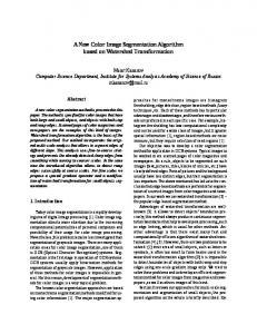
The four dimensional color image histogram is represented by two linked structures as given in Table 1 and Table 2. Actual implementation of the Table 2 may contain only m.n integer entries for JND color index, as the pixel entries are sorted spatially from left to right and from top to bottom. JND Color

R

G

B

H

X

Y

Index

JND Color Index for (xi,yi) from Table 1

1

5

15

20

335

x1

y1

1

2

10

100

20

450

x1

y2

1

3

20

50

10

470

.

.

.

.

.

.

.

.

xi

yi

K

K

25

72

90

200

.

.

.

TABLE 1: Color population

TABLE 2: Color index-pixel location relation


286


Thus Table 1 contains the R, G, B coordinates and the respective frequency information or population (H) of the tri-color stimulus, while Table 2 contains the respective color index (row index) in Table 1 and the x and y positional co-ordinates in the image. The number of rows in Table 1 is equal to the number of different color shades available in the image. In Table 1 there will be one entry for each color shade while in Table 2 there will be one entry for each pixel. The color shades which are not present in the image are not allotted any row in Table 1 and hence in Table 2. The color vectors are entered in the Table 1 in the order of their appearance in the image or in other words, as they are encountered during the scan of the image which starts from the top left corner of the image. The population (H) in Table 1 must satisfy equation (5). H = m .n − − − (5 )

∑

The proposed histogram computation procedure given below finds out the color shades available in the image and arranges them in the said format in a single scan of the complete image. Thus it does not require three scans of the complete image as in [14] neither it requires as many passes as minimum of the R,G and B frequencies as in [15]. It also simultaneously notes the positional information in a separate data structure which may further be used by different algorithms like shell clustering algorithms [16,17], which require positional information. The histogram computing algorithm with our approach has been presented below. Algorithm for Computing the Basic JND Histogram i)

ii) iii) iv)

v) vi) vii)

Initialize two data structures Table 1 and Table 2. Initialize the first entry in Table 1 by the first color vector in the image i.e. top left pixel color vector [R,G,B] and the frequency(population) by one. Initialize the first entry in Table 2 by the current row index value of Table 1 i.e. 1 , and the top left pixel position row and column i.e. y(column)=1 and x(row)=1. Also initialize a (row, column) pointer to top left corner of the image. Select a proper similarity threshold Θ1 2 2 (JNDeye ≤ Θ1≤ JNDh ) depending on the precision of vision from fine to broad as required by the application. Read the next pixel color vector in scan line order. Compare the new pixel color vector with all the previous entries in Table 1 one by one and if found similar to any of them, then accommodate it in the respective bin. Update Table 2 by entering the current index and the current row and column values and go to step v. If the new color vector is not equal to any of the previously recorded color vectors in Table 1, increment the row index of Table 1, enter the new color vector in it, set the population to 1 , make the index , row and column entry in Table 2 and go to step ii. Repeat step ii) to iv) for all the pixels in the image. Sort Table 2 in the increasing order of the color index. Save the Table 1 and Table 2 for latter analysis of the histogram. 2

The histogram computed using JNDh derived in section 2.2 as threshold, using above algorithm has miraculously reduces the colors in the natural images. The drastic reduction in number of colors in a natural image brings it to the range suitable for the machine analysis in real time. The k visually different colors in Table 1 found by the basic algorithm are further reduced using agglomeration procedure discussed in the next section.

3. HISTOGRAM AGGLOMERATION AND SEGMENTATION Agglomeration in chemical processes attributes to formation of bigger lumps from smaller particles. In the digital image segmentation, the similar pixels (in some sense) are clustered together under some similarity criteria. And thus it was inspired that the agglomeration may contribute considerably in the process of color image segmentation. In this section, a basic agglomeration histogram processing algorithm is presented. The multidimensional histogram peak detection and thresholding are complex and time consuming tasks. The agglomeration techniques can be thought of as the powerful alternatives to the other image thresholding techniques. After the compressed histogram of a real life image is obtained using the basic JND


287


histogram algorithm given in section 2, the agglomeration technique can further be used to reduce the number of colors by combining the smaller segments (less than .1% [18] of the image size) with similar colored larger segments. To implement this scheme a merging threshold Θ2 which is slightly greater than Θ1 is used, typically Θ2= Θ1+100 works well here. This stimulates the process of merging of small left over segments (after building basic JND histogram presented in section 2.3) with larger similar color segments. This helps in minimizing over segmentation. The basic agglomeration algorithm has been presented below. Algorithm for Computing Agglomerated Histogram using JND colors i) Arrange the Table 1 in decreasing order of population. ii) Starting from the first color in Table 1, compare the color with the next color in table 1. iii) If the population of the smaller segment is smaller than .1% of the image size and the two segments are similar using Θ2, merge the ith color with the previous one (the first in Table 1), their populations will be added and the color of larger population will represent the merger. iv) The merged entry will be removed from Table 1. This reduces number of rows in Table 1. In Table 2, the color index to be merged is changed by the index to which it is merged. v) Thus the first color in the Table 1 will be compared with every remaining color in Table 1 and step ii is repeated if required. vi) Step ii, iii and iv are repeated for every color in the Table 1. vii) Steps ii to v are repeated till the Table 1 does not reduce further i.e. equilibrium has reached. viii) Table 2 is sorted in ascending order of the color index. The human retina performs a low pass filtering operation following Poisson's distribution around every point on the retinal image and the neural activity initially notes and interprets the predominant or above average outputs of the retinal sensors passed to the brain via visual cortex [12]. Though we have not implemented the classical Poisson's distribution based spatial integration, the agglomeration in this work has carried out the task of low pass filtering in the color space. This reduces the number of colors in an image from several thousands to a few tens. Based on this human physiological background, the prominent segments of the image can be estimated from the agglomerated histogram. Segmentation procedure is straightforward with the data structures given in Table 1 and Table 2. In Table 2, the pixel entries are sorted spatially from left to right and from top to bottom. Segmented image can simply be formed by assigning to each pixel position a JND color from Table 1 as pointed to by the respective index in Table 2.

4. EXPERIMENTAL RESULTS In this section, we demonstrate the segmentation results of the proposed algorithm on natural images from Berkeley Segmentation Database (BSD)[19]. It Contains 300 real life RGB images of different categories and same size 481x321 pixels. It also contains benchmark segmentation results (ground truth database) of 1633 segmented images manually obtained from 30 human subjects. i.e. multiple ground truth hand segmentations of each image. For each image, the quality of segmentation obtained by any algorithm can be evaluated by comparing it with ground truth hand segmentations. The results of proposed segmentation algorithm are presented here and its effectiveness is compared with the conventional histogram based segmentation, using two quantitative measures, namely, the Probabilistic Rand Index (PRI)[20] and Peak signal to Noise Ratio (PSNR). PRI Counts the fraction of pairs of pixels whose labeling are consistent between the computed segmentation and the ground truth, averaging across multiple ground truth segmentations to account for variation in human perception. This measure takes the values in the interval [0,1]; more is better. We will consider the segmentation ‘good’ if for any pair of pixels xi, xj we would


288

Kishor Bhoyar & Omprakash Kakde Stest

Stest

Sk

like the labels of those pixels li , lj to be the same in the test segmentation if the labels li , Sk lj were the same in the ground truth segmentations, and vice versa. PSNR represents region homogeneity of the final partitioning. The higher the value of PSNR the better is segmentation. The PSNR measure [21] between the image I and the first order approximation based on the segmentation result S is calculated by equation (6). PSNR(I, S) = 10 . log

10

2 rows . columns . channels    ∑ rows ∑255columns  [I(i, j, k) −S(i, j, k)] 2 ∑ channels k  i j 

− − − −(6)

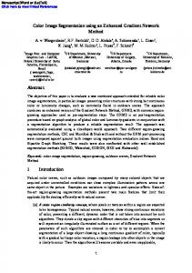
The algorithm is applied to BSD database of 300 images. The average PRI and PSNR values of all the images for two algorithms is given in Table 3. The quantitative comparison as given in Table and the qualitative (visual) comparison presented in figure 2 clearly demonstrate the superiority of proposed algorithm.

(a)

(b) FIGURE 1: Graphs showing the effect of different values of squared threshold Θ1 on average number of segments in BSD (a) and on PRI of BSD (b). The best results are obtained at Θ1=2400. Θ2= Θ1+100 for all experiments


289


The Segmentation experiments for various values of Θ1 are performed to find the best segmentation results. The Figure 1 shows the graphs plotted to analyse the performance of the proposed algorithm. The graphs shows the best performance (PRI=.7193) at value 2400 (shown 2 with vertical dotted line at Θ=2400) which is very close to the derived value of JNDh =2567. Also note that the value of average number of segments (approximately 17) at Θ1=2400 is reasonable. More the value of Θ1, less are the average number of segments and vice versa. This is obvious as increased value of Θ1 accepts more pixels as similar to given pixel and hence increases the size of the segments; thus producing lesser number of segments for any given image. From this discussion it can be concluded that we can implement fine to broad vision by varying value of Θ from JNDeye to JNDh.

Seg. Method

PRI

PSNR

Time* for Segmentation of 300 BSD images

CCH

0.7181

21.37

1.12 Hrs

JND based Color Histogram Θ=2400

0.7193

25.60

0.3575 Hrs

TABLE 3: Average Performance on BSD *On AMD Athlon 1.61 GHz processor

(a)

(PRI=0.8112, PSNR=21.3)

(PRI=0.8533, PSNR=28.16)

(PRI=0.8112, PSNR=23.30)

(PRI=0.85, PSNR=28.11)

(b)

( c)

FIGURE 2: Few Segmentation results on BSD database: Column (a) Original Images, Column (b) CCH Segmented images, and Column (c) Segmented images with proposed approach.


290


5. CONCLUSION AND FUTURE WORK Observing the graphs given in Figure 1, the effect of squared threshold Θ1 on JND Histogram based Segmentation can be summarized as follows. It is observed that as Θ1 increases; average number of segments (Avgk) over BSD exponentially decreases. As Θ1 increases, PRI decreases. Optimal value of Θ1 (considering both Avgk and PRI) should be around 2567. It is observed that 2 the results on Segmentation on natural images in BSD are optimal near JNDh =2400. This approves our claim on derived value of JND for RGB color space. The result comparison of JND Histogram Segmentation approach with CCH based segmentation approach on BSD images is summarized in Table-3. It can be observed that the proposed segmentation approach outperforms CCH in terms of PRI as well as PSNR. Also note the reduction in time required to perform the segmentation of all the 300 images in the database, with the proposed approach. The information obtained about number of segments, and their cluster centers can be used to initialize Fuzzy C-means Segmentation algorithm. In future work we are proposing a modified FCM segmentation algorithm that works with the histogram bins as data for clustering instead of individual pixel values.

6. REFERENCES 1. 2. 3.

4. 5. 6. 7. 8. 9. 10. 11. 12. 13.

M.Swain and D. Ballard,”Color indexing”, International Journal of Computer Vision, Vol.7, no. 1,1991. W. Hsu, T.S. Chua, and H. K. Pung, “An Integrated color-spatial approach to Content-Based Image Retrieval”, ACM Multimedia Conference, pages 305-313, 1995. Ka-Man Wong, Chun-Ho Chey, tak-Shing Liu, Lai-Man Po, “Dominant color image retrieval using merged histogram”, Circuits and Systems,ISCAS’03 Proceedings of 2003 International Symposium, Vol. 2, pp II-908 – II-911, 2003 Ju Han and Kai-Kuang Ma, ”Fuzzy color Histogram and its use in color image retrieval”, IEEE Transactions on Image Processing, Vol. 11, No. 8, 2002. Cheng, H.D., Jiang, X.H., Sun, Y., Wang, J., “Color image segmentation: Advances and prospects”, Pattern Recognition 34,2259–2281, 2001. Liew, A.W., Yan, H., Law, N.F., “Image segmentation based on adaptive cluster prototype estimation”, IEEE Trans. Fuzzy Syst. 13 (4), 444–453, 2005. Pal, N.R., Pal, S.K., “A review on image segmentation techniques”, Pattern Recognition 26 (9), 1277–1294, 1993. Aghbari, Z. A., Al-Haj, R., “Hill-manipulation: An effective algorithm for color image segmentation”, Image Vision Comput. 24 (8), 894–903, 2006.. Cheng, H.D., Li, J., “Fuzzy homogeneity and scale-space approach to color image segmentation”, Pattern Recognition 36, 1545–1562, 2003. Gaurav Sharma, “Digital color imaging”, IEEE Transactions on Image Processing, Vol. 6, No.7, , pp.901-932, July1997. K. M. Bhurchandi, P. M. Nawghare, A. K. Ray, “An analytical approach for sampling the RGB color space considering limitations of human vision and its application to color image analysis”,, Proceedings of ICVGIP 2000, Banglore, pp.44-49. A. C. Guyton, “A text book of medical Physiology”, W.B.Saunders company, Philadelphia, pp.784-824, (1976). A. Moghaddamzadeh and N. Bourbakis, “A fuzzy region growing approach for segmentation of color images”, Pergamon,Pattern Recognition, Vol.30,No.6, pp.867-881, 1997.


291


14. Sang Ho Park, Il Dong Yun and Sang Uk Lee, “Color image segmentation based on 3-D clustering: morphological approach”, Pergamon, Pattern Recognition, Vol.44, No.8, pp. 1061-1076, 1998. 15. Liang-Kai Huang and Mao-Jiun J.Wang, “Image thresholding by minimizing the measures of fuzziness”, Pergamon,Pattern Recognition, Vol.28,No.1, pp.41-51, 1995. 16. Raghu Krishnapuram, Hichem Frigui and olfa Nasraoui, “Fuzzy possiblistic shell clustering Algorithms and their application to boundary detection and surface approximation- part I”, IEEE Transactions on Fuzzy Systems, Vol.3,No.1, pp.29 -43, February1995. 17. Raghu Krishnapuram, Hichem Frigui and olfa Nasraoui, “Fuzzy possiblistic shell clustering Algorithms and their application to boundary detection and surface approximation- part II”, IEEE Transactions on Fuzzy Systems, Vol.3,No.1, pp.44-60, February1995. 18. Milind M. Mushrif, Ajoy K. Ray,”Color image segmentation:Rough-set theoretic approach” ,Elsevier Pattern Recognition Letters, pp 483-493,2008. 19. D. Martin, C. Fowlkes, D. Tal, J. Malik, “A database of human segmented natural images and its application to evaluating segmentation algorithms and measuring ecological statistics”, Proceedings of IEEE International Conference on Computer Vision, 2001, pp.416 –423 20. R. Unnikrishnan, M. Hebert, “Measures of Similarity”, IEEE Workshop on Computer Vision Applications, pp. 394–400, , 2005. 21. D. Suganthi, S. Purushothaman, ”IMRI Segmentation using echo state neural network”, International Journal of Image Processing, Volume (2):Issue (1), pp 1-9.


292