JOURNAL OF IMAGING SCIENCE AND TECHNOLOGY® • Volume 46, Number 3, May/June 2002
Modeling Ink Spreading for Color Prediction Patrick Emmel▲ Clariant International, Masterbatches Division, Muttenz, Switzerland
Roger David Hersch▲ Ecole Polytechnique Fédérale de Lausanne (EPFL), Département d’Informatique, Laboratoire de Systèmes Périphériques, Lausanne, Switzerland
This study aims at modeling ink spreading in order to improve the prediction of the reflection spectra of three ink color prints. Ink spreading is a kind of dot gain which causes significant color deviations in ink jet printing. We have developed an ink spreading model which requires the consideration of only a limited number of cases. Using a combinatorial approach based on Pólya’s counting theory, we determine a small set of ink drop configurations which allows us to deduce the ink spreading in all other cases. This improves the estimation of the area covered by each ink combination that is crucial in color prediction models. In a previous study, we developed a unified color prediction model. This model, augmented by the ink spreading model, predicts accurately the reflection spectra of halftoned samples printed on various ink jet printers. For each printer, the reflection spectra of 125 samples uniformly distributed in the CMY color cube were computed. The average prediction error between measured and predicted spectra is about ∆Ε = 2.5 in CIELAB. Such a model simplifies the calibration of ink jet printers, as well as their recalibrations when ink or paper is changed. Journal of Imaging Science and Technology 46: 237–246 (2002)
Introduction In previous publications, 1,2 we presented a color prediction model for halftoned samples which is based on a new mathematical formulation of the Kubelka–Munk equations. This new model requires, like Neugebauerbased methods,3 an estimation of the area covered by each ink density combination. This estimation needs to be computed by simulating the printing process. In ink jet printing, the superposition of ink drops causes a significant dot gain, i.e., a change of the covered area (see Fig. 1). When ink drops are printed one over another or just partially overlap, an ink spreading process takes place. This phenomenon results from a complex physical interaction between the ink drops and the surface of the printed media. Changing the inks or the paper modifies the magnitude of the spreading and induces color prediction errors ranging up to ∆Ε = 20 in CIELAB. According to observations made under the microscope, the spreading depends on the state of the surface (“wet” or “dry”) and the configuration of the neighboring impacts. In our previous study,2 we analyzed samples made of two ink layers, and deduced a set of empirical rules describing the enlargement of the impact of an ink drop. For each ink–paper combination twelve enlargement coefficients were estimated by observing samples un-
Original manuscript received December 12, 2000 ▲ IS&T Member Tel: +41 61 469 6187 ; Fax: +41 61 469 6597; email:
[email protected] [email protected] ©2002, IS&T—The Society for Imaging Science and Technology
der the microscope. This approach lead to accurate color predictions but it has two major drawbacks: firstly, the simulated dot shapes are not realistic; secondly, the number of different configurations and the number of enlargement coefficients increases dramatically with the number of ink layers. Therefore, a new investigation method is proposed. It is based on an impact model whose shape changes as a function of the configuration of the neighboring impacts and of the state of the surface. Because the number of configurations is high, Pólya’s counting theory is used to find a reduced set of cases whose analysis allows us to deduce the spreading in all other configurations. By building samples with this reduced set, standard measuring instruments can be used to estimate the ink spreading. This information will be used by our color prediction model in order to compute accurately the spectra of printed samples. The Impact Model In our color prediction software,2 high resolution grids model the printed surface. One grid is used for each ink. The value of a grid point corresponds to the local amount of a given dye (see Fig. 2). The density profile of an isolated ink impact was measured under a microscope and approximated by a parabolic function.4 The resulting ink impact model (see Fig. 2) is used as a stamp. Wherever an ink drop hits the surface of the printed media, the impact model is stamped at the same location on the high resolution grid. Stamp overlapping is additive. In a color print using n inks, the ink combination covering a surface element at position (x, y) is given by the set of n values of the grid points (x, y) in the n superposed high resolution grids. The area covered by
237
Paper
Cyan cluster
Green cluster
Yellow ink
(a) (b) Figure 1. Microscopic views of a halftoned cyan sample (a) and of a green halftoned sample (b). The green sample (b) is made of the same cyan layer as (a) and covered with a uniform yellow layer. Note the enlargement of the cyan clusters in (b).
a given combination of n inks is estimated by counting the number of surface elements having the same set of n values. In ink jet printing, the shape of an impact highly depends on the configuration of the neighboring ink drop impacts and on the state of the surface. Therefore we need to extend the traditional circular or elliptic impact model 5 to more sophisticated shapes. Most ink jet printers use a hexagonal grid when printing in color. Hence, each impact has six neighbors. Therefore, the circumference of an impact is parameterized by six vectors having a common origin at the impact center. Each vector is oriented to the direction of the midpoint between two neighboring impacts (see Fig. 3). Let us denote r i(1 ≤ i ≤ 6) the length of the vector which is oriented in the direction given by the angle θi = π/6 + (i – 1) · π/3. The shape of the impact is approximated by a parametric curve that joins the vertices defined by the six vectors. Let us denote ρ = r(θ) the equation in polar coordinates of this parametric curve. Because we assume that a neighbor influences only locally the shape of the impact, the parametric curve depends only on ri and ri+1 when θi ≤ θ ≤ θi+1. In order to get realistic impact shapes, we interpolate the values of the radius ρ between ri and r i+1 by using a polynomial of degree three: ρ = r(θ) = 2(r i – r i+1)t3 – 3(ri – r i+1)t 2 + r i where t=
π 3 θ − − i π 6
(1)
Note that
π π r + i ⋅ = ri , 6 3 and that the derivative
π dr π + i ⋅ = 0. 3 dθ 6 These properties guarantee the continuity of r(θ) and of its first derivative. We assume that the density D at the location defined by the polar coordinates (ρ, θ) (0 ≤ ρ ≤ r(θ)) is given by: ρ D(ρ, θ ) = DM ⋅ 1 − r (θ )
238 Journal of Imaging Science and Technology®
(2)
where DM is the density at the center of the impact. Note that a circular impact (r(θ) constant) has a parabolic density profile as observed in our previous study.4 The amount of dye remains constant during the spreading process, only the spatial distribution is changed. Therefore, the maximal density D M at the center of the impact must decrease when the impact is enlarged. By integrating Eq. (2) over the area occupied by the impact, we get the total amount of dye within the impact (see Appendix). Because this amount must remain constant, we get the following equation for DM:
and
π π π π + (i − 1) ⋅ ≤ θ ≤ + i ⋅ . 6 3 6 3
2
DM
= D0 ⋅ 6 ∑ i=1
6 r02 13 2 + ⋅ − ( ) r r r r i i + 1 140 i i + 1
(3)
Emmel and Hersch
Figure 3. Six vectors define the circumference of the impact. The dashed circles indicate the locations of neighboring impacts.
Figure 2. High resolution grid modeling the printed surface. The value of a grid point corresponds to the local amount of dye. The density profile of an isolated ink impact is parabolic.
where r0 and D0 are respectively the radius and the maximal density at the center of an isolated circular impact which did not spread. This new impact model allows us to simulate the spreading by changing the six ri coefficients according to the configuration of the neighbors and the state of the surface. Pólya Counting In this section, we derive the number of non-equivalent ink-drop configurations with the help of Pólya’s “counting theory.” (Readers interested mainly in the final ink spreading model may skip over this section.) Pólya’s counting requires three steps: first, defining the group of symmetries acting on the set of corners, second, factorizing each permutation into cycles, and third, calculating the cycle index polynomial. As we pointed out in the previous section, most ink jet printers use a hexagonal grid when printing in color. So
Modeling Ink Spreading for Color Prediction
Figure 4. There are six rotations and six reflections that bring a regular hexagon onto itself.
each impact has six neighbors whose centers are the corners of a regular hexagon. In a three-ink color print, each pixel of the printed surface is in one of the following four states: no ink, covered with one ink drop, covered with two ink drops or covered with three ink drops. Because an impact has six neighbors, there are 46 = 4096 possible neighbor configurations. On the considered center point, a new ink drop is printed on a surface that is in one of the following three states: dry (no ink), covered with one ink drop or covered with two ink drops. Therefore, there are 3 × 46 = 12288 configurations to consider. Among these 12288 configurations, many are equivalent by reflection or by rotation. Note that there are
Vol. 46, No. 3, May/June 2002 239
twelve symmetries that bring a regular hexagon onto itself: six rotations and six reflections (see Fig. 4). By considering only non-equivalent configurations, the number of cases to analyze can be reduced. At the beginning of the century, the mathematician George Pólya developed a theory for this kind of counting problem. 6 Later, his work was translated into English7 and became known in the mathematical literature as “Pólya’s counting theory.” In the forthcoming discussion, we present only how to apply this theory to our problem. Good presentations of Pólya’s counting theory can be found in textbooks. 8 As mentioned above, there are twelve geometric motions, six rotations and six reflections, which act as permutations of the corners of the regular hexagon. Let us denote ρ06, ρ16, ρ26, ρ36, ρ46 and ρ56 the rotations by an angle of θ = 0, θ = π/3, θ = 2π/3, θ = π, θ = 4π/3 and θ = 5π/3 respectively. Furthermore, we denote τad, τ be, τcf, the reflections whose axes are the lines (ad), (be), (cf) respectively, and τab, τbc, τcd, the reflections whose axes are the mediators of the segments [ab], [bc], [cd] respectively. This set of twelve symmetries with the composition operation has a group structure:9 the unit element is ρ06, each symmetry has an inverse, and the composition of two symmetries is still a symmetry. Let us denote this group D 6. The group is acting on the set of corners of the hexagon. By applying the same operation, one of the symmetries listed in Table I, iteratively to the hexagon, the corners follow cyclic trajectories. After a finite number of iterations, each corner gets back to the starting point. For instance, by applying iteratively the rotation ρ26 to the corner (a) of Fig. 4, we get the cycle [a, c, e]: a is first moved to c, then to e, and finally comes back to a. Note that for a given symmetry, an individual corner belongs only to one cycle. A classical result from group theory shows that each element of D6 acting on the set of corners of the hexagon can be factorized into disjoint cycles.10 The factorizations of the elements of D6 are listed in the second column of Table I. The reflection τcf, for example, is factorized into two cycles of one corner ([c] and [f]) and two cycles of two corners ([a, e] and [b, d]). Let the variable z i correspond to a cycle having i corners. To each symmetry we associate a monomial that is the product of the (z i)’s according to the cycle factorization as shown in the third column of Table I. The reflection τcf is associated with z1· z1 · z 2 · z 2 = z 21z 22. The sum of the monomials divided by the number of the symmetries of the group D6 is called the cycle index:
P( z1, z2 , z3 , z6 ) =
(
)
1 ⋅ z16 + 2 z6 + 2 z32 + 4 z23 + 3 z12 z22 (4) 12
Let us denote k be the number of states in which a corner can be. According to Pólya’s theory,11 the number of non-equivalent hexagons is:
(
1 P( k, k, k, k) = ⋅ k6 + 2 k + 2 k 2 + 4 k3 + 3 k 4 12
)
(5)
Therefore, the number of non-equivalent configurations of six neighboring ink drop impacts being in one of k states is given by P(k, k, k, k). Furthermore, a new drop is printed on a surface which is in one of (k – 1) states. So finally, the total number of non-equivalent configurations is:
N = (k − 1) ⋅ P (k, k, k, k)
240 Journal of Imaging Science and Technology®
(6)
TABLE I. Cycle Factorizations and Monomials of the Group D6 Acting on the Corners of the Hexagon Symmetry
Cycle factorization
Monomial
ρ ρ 16 ρ 26 ρ 36 ρ46 ρ 56 τad τbe τcf τab τbc
[a], [b], [c], [d], [e], [f], [a,b,c,d,e,f] [a,c,e], [b,d,f] [a,d], [b,e], [c,f] [a,e,c], [b,f,d] [a,f,e,d,c,b] [a], [d], [b,f], [c,e] [b], [e], [a,c], [d,f] [c], [f], [a,e], [b,d] [a,b], [c,f], [d,e] [b,c], [a,d], [e,f]
z 61 z6 z 23 z 32 z 23 z6 z 21z22 z 21z22 z 21z22 z 32 z 32
τcd
[c,d], [a,f], [b,e]
z 32
0 6
In color prints using three inks, we have k = 4 states (no ink, one ink drop, two ink drops, three ink drops). Hence the number of non-equivalent configurations is N = 1290. In four-ink printing (k = 5), N rises to 6020. Note that for two inks k = 3 and N drops to 184. Other geometric shapes, as for instance non-regular hexagons, are mapped onto themselves by other groups of symmetries. But the same procedure can be applied to find the number of non-equivalent configurations. A Simplified Model of Ink Spreading The spreading process is a complex interaction between the inks and the printed surface. It is strongly related to physical properties like wettability and solvent absorption. Therefore the inks behave differently on every surface. Furthermore, the number of cases in three-ink-printing (N = 1290) is too large for performing exhaustive measurements. We propose a simplified model of ink spreading. First, the geometry of the problem is simplified.12,13 The hexagon is subdivided into six triangles which share the center O of the hexagon as a common vertex (see Fig. 5). Second, the spreading in the direction of the mediator of the segment [a, b] is supposed to depend only on the state of the neighbors located in a and b, and the state of the surface at the center O of the hexagon. This simplified geometry allows to define a group S of symmetries acting on the segment [a, b], because only a and b play equivalent roles in the triangle (a, O, b). The group S has two elements: ρ0 the rotation by the null angle, and the reflection τab whose axis is the mediator of the segment [a, b]. The cycle factorizations and the monomials of the group S are listed in Table II. The cycle index is:
P( z1, z2 ) =
(
1 ⋅ z12 + z2 2
)
(7)
Finally, the total number of non-equivalent configurations is given by combining Eq. (6) and Eq. (7): N = (k − 1) ⋅ P (k, k) =
(k − 1) ⋅ k ⋅ (k + 1) 2
(8)
where k is the number of states of a neighbor. According to Eq. (8), in two-ink-printing (k = 3) we must consider N = 12 cases; in three-ink-printing (k = 4), we must consider N = 30 cases; and in four-ink-printing (k = 5), we must consider N = 60 cases.
Emmel and Hersch
TABLE II. Cycle Factorizations and Monomials of the Group S of Symmetries Acting on the Segment [a, b] Symmetry
Cycle factorization
Monomial
ρ0
[a], [b]
z12
τab
[a,b]
z2
Figure 5. A simplified geometry: the hexagon is subdivided into six triangles that share the center of the hexagon as a common vertex. The spreading of the ink drop impact in the direction of the mediator of [a, b] depends only on the state of O, a, and b.
These sets of cases are small enough for performing exhaustive measurements in order to calibrate the ink spreading model. From each case, we can deduce the value of a coefficient ri , which is used by our previously defined impact model. The shape of a simulated impact depends on six r i coefficients which are related to the configuration of the neighboring impacts and the state of the surface. Enumerating the Configurations Pólya’s counting theory gives the number of configurations that must be considered in order to calibrate the ink spreading model. The configurations themselves are computed by other means. Powerful generating algorithms exist,14 but for the sake of simplicity, a naive sieve method is used. A computer generates the list of all configurations. Considering the first configuration, all equivalent configurations are removed from the list. The computer applies this procedure to the next configuration of the list until the end of the list is reached. The 30 non-equivalent configurations for three-ink-printing are listed in Fig. 6. Prediction Results and Discussion The new ink spreading model was combined with our color prediction method2 in order to predict the spectra of two series of 125 samples uniformly distributed in the CMY color space. Each series is a set of 5 × 25 samples printed on five sheets of paper. The area coverage of the yellow ink is constant for all samples printed on the same sheet, and varies from sheet to sheet. The first series was printed on Epson Glossy Photo Quality Paper using an Epson Stylus-Color™ printer which is based on a piezo electric technology,15 and the second series was printed on HP Photo Paper, using an HPDJ560C printer which is based on conventional thermal ink jet techniques.16 All samples were produced with a clustered dither algorithm with 33 tone levels.
Modeling Ink Spreading for Color Prediction
Figure 6. List of the 30 non-equivalent configurations in a three-ink print. The dashed circles indicate the locations of neighbors that are not covered with ink. The white disks correspond to one ink drop, the gray disks correspond to two ink drops, and the black disks correspond to three ink drops. The vectors indicate the orientation of the spreading. The third and sixth columns indicate which test-sample is used to determine the spreading coefficient.
For both series, the radius r0 of an isolated circular impact was measured accurately under the microscope. In the HP series, the superposed cyan, magenta and yellow ink drop impacts have almost the same size, whereas in the Epson series, the radius of the yellow drop impact is 20% larger than the radius of the cyan drop impact, which is, in turn, is 30% larger than the radius of the magenta drop impact.
Vol. 46, No. 3, May/June 2002 241
TABLE III. Prediction Results in CIELAB ∆ E and ∆E 94 for the Epson Series Series of constant yellow ink percentage 0% 25% 50% 75% 100%
2
∆E
∑ ∆E n
1.67 1.81 1.95 2.91 2.85
1.97 1.96 2.14 3.02 3.11
Maximal ∆E
∆E 94
∑ ∆E94 n
3.58 3.11 4.13 5.59 5.75
0.95 1.10 1.24 1.85 1.96
1.14 1.22 1.34 1.97 2.16
2
Maximal ∆E 94 2.49 2.37 2.46 3.56 3.93
TABLE IV. Prediction Results in CIELAB ∆ E and ∆E 94 for the HP Series Series of constant yellow ink percentage 0% 25% 50% 75% 100%
Figure 7. List of the ten test patterns used to determine the spreading coefficients. The dashed circles indicate the locations of neighbors that are not covered with ink. The white disks correspond to one ink drop, the gray disks correspond to two ink drops, and the black disks correspond to three ink drops. Each test-sample is used to determine one or two spreading coefficients whose numbers are given in the third column. Note that the spreading coefficients of the configurations 1, 2, 11, 13, 14, 15 must be determined prior to 12, and that the spreading coefficients of the configurations 21, 23, 26, 27, 28, 29 must be determinated prior to 22, 24, 25.
242 Journal of Imaging Science and Technology®
2
∆E
∑ ∆E n
2.07 2.57 2.59 3.27 3.92
2.34 2.85 2.90 3.49 4.28
Maximal ∆E
∆E 94
∑ ∆E94 n
4.70 4.85 5.48 6.85 6.89
0.96 1.19 1.34 1.97 2.45
1.06 1.28 1.52 2.13 2.68
2
Maximal ∆E 94 1.89 2.64 3.65 4.13 4.14
For each ink drop configuration, the corresponding radius vector length ri is estimated by indirect means. We observed that a given ink drop spreads only if the local amount of solvent is higher than the amount of solvent at the neighbor’s location. Therefore we assume that there is no spreading in the following configurations: 3, 4, 5, 6, 7, 8, 9, 10, 16, 17, 18, 19, 20, and 30 (see Fig. 6). Considering the other configurations we define ten test samples, each of which being a mosaic composed of a single pattern as shown in Fig. 7. Note that the dot geometry of the test samples has been chosen to correspond to the dot geometry of the clustered halftoning algorithm being used. For example, test samples (a) and (c) given in Fig. 7 correspond to the samples shown in Fig. 1a and in Fig. 1b respectively. Each test sample is used to determine one or two ink spreading coefficients r = ri/r0. In other words, a given test sample contains several occurences of one or two dot configurations whose spreading coefficients are unknown. All test samples are printed and measured. For each test sample several simulation iterations are required to fit the predicted and the measured reflection spectrum by varying the values of the radius vectors lengths r i. The ink spreading coefficients r = ri/r0 computed for each series are given in Fig. 8. Note that the ink spreading coefficients for the Epson series are given for the magenta drop impact. Using our prediction model and its extension for fluorescent substances 17 (the magenta ink of the HewlettPackard printer being fluorescent), we computed the spectra of 250 samples, and compared them with the spectra measured under a tungsten light source whose relative radiance spectrum is given in Fig. 9. The CIELAB values of all samples were computed for the 2° standard observer. The average colorimetric deviation between measured and predicted spectra of the Epson series and of the HP series are given in Table III and Table IV respectively. The results obtained for the Epson series are a little better than the results for the HP se-
Emmel and Hersch
Figure 8. Spreading of HP inks printed on HP paper and spreading of Epson inks printed on Epson paper. For each of the 30 nonequivalent configurations in a three-ink print, the spreading coefficients r = r i/r0 are respectively given in the columns entitled HP and Epson. The second and sixth columns show the dot configurations. The dashed circles indicate the locations of neighbors that are not covered with ink. The white disks correspond to one ink drop, the grey disks correspond to two ink drops, and the black disks correspond to three ink drops. The vectors indicate the orientation of the spreading.
ries. This could be due to the stronger spreading of the HP inks. In order to show how our ink spreading model improves color prediction, we consider the 25 samples of the series having a 100% coverage of yellow ink and which are printed on HP Photo Paper with an HP DJ560C printer. The prediction results corresponding to this series are given in the last row of Table III. The measured and computed spectra of the 25 samples are converted into CIE-XYZ values that are shown in a graphical form in Fig. 10. Figure 10a shows the deviation between measured and computed colors taking ink spreading into account; and Fig. 10b shows the deviation between measured and computed colors without taking ink spreading into account. Without taking ink
Modeling Ink Spreading for Color Prediction
spreading into account, the prediction error is higher than ∆E = 10 in CIELAB for samples made of more than two inks, because printing ink drops one over another significantly increases ink spreading. The spectra of samples made with only one ink are well predicted because almost no ink spreading occurs. The measured and predicted spectra of the cyan and green samples shown respectively in Fig. 1a and Fig. 1b are given in Fig. 11a and Fig. 11b. Sample (b) is made of the same cyan layer as sample (a) and covered with a uniform yellow layer. In spite of the absence of absorption of the yellow ink at 630 nm, the measured reflection coefficient of sample (b) is lower than that of sample (a) at this wavelength (compare Fig. 11b and Fig. 11a). This difference is explained by ink spreading. The cyan
Vol. 46, No. 3, May/June 2002 243
1.75
0.25
550
600
650
700
Figure 9. Relative radiance spectrum of the tungsten light source.
80
Yellow
60
Y
40
Green 20
0
Red
0
20
40
60
80
X (a) (b) Figure 10. Projection onto the XY plane within the CIE-XYZ color space of the deviations between computed and measured colors of 25 samples having a 100% coverage of yellow ink, and which are printed on HP photo paper using an HP DJ560C printer. Each dot indicates the measured color, and the other end of the segment indicates the computed color: (a) shows the color deviation when ink spreading is taken into account;, (b) shows the color deviation when ink spreading is not taken into account.
ink covers a larger area with a lower density, and therefore produces a higher light absorption. Note that in the case of sample (b), the prediction error is ∆E = 9.2 in CIELAB if ink spreading is not taken into account. Conclusions We introduce a new method for investigating ink spreading. The spreading process is modeled by enlarging the drop impact according to the configuration of its neighbors and the state of the surface. The number of cases that must be analyzed is reduced to a small set by using Pólya’s counting theory. In a three-ink-
244 Journal of Imaging Science and Technology®
printing process, only 30 cases must be considered instead of 3 × 4 6 = 12288. The printing process is simulated by stamping impacts of different shapes on high resolution grids. Each shape is determined by 6 radii. The value of each radius is estimated by fitting the reflection spectra of ten test samples in several simulation iterations. This allows us to compute the relative areas occupied by the various ink combinations in a three-ink process. We predict accurately the spectra of 250 samples produced by two different printers. The average prediction error is about ∆E = 2.5 and the maximal error is less than ∆E = 7 in CIELAB.
Emmel and Hersch
nm (a)
nm (b) Figure 11. Measured spectra (continuous lines) and predicted spectra (dashed lines): (a) of the halftoned cyan sample shown in Fig. 1a (25% cyan ink coverage), and (b) of the green sample shown in Fig. 1b (superposition of a cyan layer at 25% ink coverage and a yellow layer at 100% ink coverage). Note that the reflection coefficient of sample (b) is lower than that of sample (a) at 630 nm in spite of the absence of absorption of the yellow ink at this wavelength.
In our view the proposed ink spreading model may considerably increase the accuracy of existing advanced color prediction models.18 It may also be used for improved Neugebauer-based color prediction methods 3 because they require an accurate estimation of the area covered by each ink combination. Appendix: Total Amount of Dye Within an Ink Drop Impact The density profile of an ink drop impact is given by Eq. (2). The total amount T of dye within an ink drop impact is obtained by integrating Eq. (2) over the area covered by the impact:
T=
2π
∫ ∫ 0
r (θ )
0
DM
ρ 2 ⋅ 1 − ρ dρ dθ r (θ )
T=
π ⋅ D0 ⋅ r02 2
(10)
Let us now consider an ink drop that spread. In this case, r(θ) is defined piecewise as shown in Eq. (1). The integral in Eq. (9) can be written:
T=
6
θ i+ 1
r (θ )
∑ ∫θ ∫0 i=1 i
(9)
During the spreading process, the amount of dye T remains constant. We can establish a relationship between the maximal density D0 at the center of a drop
Modeling Ink Spreading for Color Prediction
that did not spread, and the density DM at the center of a drop that spread, by calculating T in both cases. Within an isolated circular impact (r(θ) = r 0) which did not spread (DM = D 0), the total amount of dye is:
DM
ρ 2 ⋅ 1 − ρ dρ dθ r (θ )
(11)
where
θi =
π π + (i − 1) ⋅ . 6 3
Vol. 46, No. 3, May/June 2002 245
By integrating in Eq. (11) with respect to variable ρ, we get: T = DM
6
θ i+ 1
∑ ∫θ i=1
i
[ r (θ )]2 dθ . 4
(12)
In the next step, the following change of variable is performed: t = (3/π) (θ – π/6) – i. The integral (12) can be written:
T=
π ⋅ DM 12
6
∑ ∫0 i=1
1
[2(r − r
i + 1 )t
i
3
− 3(ri − ri + 1 )t 2 + ri
] dt . (13) 2
By integrating Eq. (13) with respect to the variable t, we get: T=
π ⋅ DM 12
6
∑
i=1
13 ⋅ (ri − ri + 1 ) 2 ri ri + 1 + 140
(14)
Finally, by combining Eqs. (10) and (14) we obtain Eq. (3). Acknowledgment. We would like to thank Dr. Rita Hofmann from Ilford Imaging for providing useful information on ink jet paper, and the Swiss National Science Foundation (grant No. 21-54127.98) for supporting the project.
246 Journal of Imaging Science and Technology®
References 1. P. Emmel and R. D. Hersch, Towards a Color Prediction Model for Printed Patches, IEEE Computer Graphics and Applications, 19 (4) 54–60 (1999). 2. P. Emmel and R. D. Hersch, A Unified Model for Color Prediction of Halftoned Prints, J. Imaging Sci. Tech. 44, 351–359 (2000). 3. R. Rolleston and R. Balasubramanian, Accuracy of Various Types of Neugebauer Model, Proceedings of the First IS&T/SID Color Imaging Conference, IS&T, Springfield, VA, 1993, pp. 32–37. 4. P. Emmel, Modèles de Prédiction Couleur Appliqués à l’Impression Jet d’Encre , PhD thesis No. 1857, Ecole Polytechnique Fédérale de Lausanne (EPFL), Lausanne, Switzerland, 1998, p. 114, http:// diwww.epfl.ch/w3lsp/publications/colour/thesis-emmel.html (in French). 5. C. J. Rosenberg, Measurement-based evaluation of a printer dot model for halftone algorithm tone correction, J. Electronic Imaging 2(3), 205– 212 (1993). 6. G. Pólya, Kombinatorische Anzahlbestimmungen für Gruppen, Graphen und chemische Verbindungen, Acta Mathematica, 68, 145–254 (1937). 7. G. Pólya and R. C. Read, Combinatorial Enumeration of Groups, Graphs and Chemical Compounds, Springer, New York, 1987. 8. R. A. Brualdi, Introductory Combinatorics, Third Edition, Prentice Hall, London, 1999, pp. 546–586. 9. S. Lang, Algebra, Third Edition, Addison-Wesley, New York, 1995, p. 7. 10. Ref. 9, p. 30. 11. R. A. Brualdi, Introductory Combinatorics, Third Edition, Prentice Hall, London, 1999, p. 575. 12. S. Wang, Algorithm-Independent Color Calibration for Digital Halftoning, Proceedings of the Fourth IS&T/SID Color Imaging Conference, IS&T, Springfield, VA, 1996, pp. 75–77. 13. S. Wang and C. Hains, US Patent No. 5,748,330 (1998). 14. J. Sawada, Fast Algorithms to Generate Restricted Classes of Strings Under Rotation, PhD Thesis, University of Victoria, Canada, 2000. 15. http://www.epson.com/ 16. http://www.hp.com/ 17. P. Emmel and R. D. Hersch, Spectral Color Prediction Model for a Transparent Fluorescent Ink on Paper, Proceedings of the 6th IS&T/SID Color Imaging Conference, IS&T, Springfield, VA, 1998, pp. 116–122. 18. G. Rogers, A Generalized Clapper-Yule Model of Halftone Reflectance, Color Res. Appl. 25, (6) 402–407 (2000).
Emmel and Hersch