Colour image representation using BSP tree. - CiteSeerX

COLOR IMAGE REPRESENTATION USING BSP TREE S SUDIRMAN and Guoping QIU School of Computer Studies The University of Leeds, Leeds LS2 9JT United Kingdom [email protected] [email protected]

ABSTRACT This paper presents a novel approach to colour image representation using Binary Space Partitioning (BSP) Tree. In the past, BSP tree has been used to represent grey scale images. Extending the method to colour images is however not straightforward. We propose to apply the moment-preserving thresholding technique to binarize the colour image, and determine the partitioning lines from the binary image based on a goodness-of-fit criterion. We present the results of this new technique and its applications to image coding. We also discuss the potential of the application of the technique to content based image indexing and retrieval.

Keywords: BSP Tree, segmentation, representation, moment preserving thresholding, coding and indexing.

1

INTRODUCTION

Image representation has been a popular research area for the past few years. Recent approaches to represent images can be found in [4],[7],[9],[12]. Although it is evident that one of the driving forces in image representation research is to efficiently coding the image, it is not suggested until recently [6] that this area has a significant potential for content access application in the representation domain. This paper presents a novel approach to colour image representation based on Binary Space Partitioning (BSP) Tree [1]. In the past, BSP tree has been used as an efficient representation of grey scale images [7]. In this paper we use the same principle of constructing the BSP tree and extend the ideas to color images by applying the moment-preserving thresholding technique [5][11] to binarize the colour image, and determine the partitioning lines from the binary image based on a goodness-of-fit criterion. The use of moment-preserving technique in image processing has attracted some researchers in recent years. Tabatabai and Mitchell [10] proposed an edge detection technique based on fitting the first three greylevel moments to the input data and computing edge

location. Tsai [11] developed a moment-preserving thresholding technique for image segmentation purposes. In a survey paper [8] Tsai's segmentation method was reported to have a good performance when compared to other thresholding techniques. Tsai and Yang [13] and Pei and Cheng [5] used the moment-preserving thresholding technique to detect edges in colour images. The latter generalised the 3-dimension complexity of digital color representation in the form of quaternions. The method proposed in this paper uses this technique in processing the color data.

2

MOMENT PRESERVING THRESHOLDING

The original idea of moment-preserving thresholding technique [11] was designed for grey-level image and is briefly reviewed here. Given a grey-scale image f with N number of pixels and its grey-level value at ( x , y ) denoted by f ( x , y ) , the ith grey-moment is calculated as: 1 mi = ∑∑ f i ( x , y ) i = 0,1,2,... (1) N x y Let F ( f ) → g be a function that operates on f such that the 1 st to the ith moment of g are equal to the 1st to the ith moment of f respectively. Then F is said to preserve up to the ith moment of the input data in the output data. Arguably the more moments the operator preserves the more information of the input image is retained in the output image [13]. The output image g has only two grey-level values h0 and h1 which correspond to the pixels which values are below and above a threhold T respectively. In order to preserve the moment of the input image in the output image the following constraints have to be met: p 0 + p1 = 1 (2) p 0 h 0k + p 1 h1k = m k k ≤i (3) where i is the maximum order of moment to be preserved and p 0 and p1 denote the fraction of pixels having grey values h0 and h1 respectively.

© International Conference on Color in Graphics and Image Processing - CGIP’2000

Pei and Cheng [5] extended the idea to color image using quaternion numbers. The algebra of quaternions is the generalisation of complex numbers [2]. The threedimensional data set (R,G,B) of color images can be represented as a quaternion numbers qˆ (n ) : qˆ (n ) = q 0 (n ) + q1 (n ) ⋅ i + q2 ( n ) ⋅ j + q 3 (n ) ⋅ k (4) where q 0 (n ) = 0, q 1 (n ) = R, q 2 (n ) = G , q 3 ( n ) = B The 3 quaternion moments are defined as follows: mˆ 1 = E [qˆ] mˆ 2 = E [qˆ ⋅ qˆ*] mˆ 3 = E [qˆ ⋅ qˆ * ⋅qˆ ] where qˆ * and E[qˆ] are the complex conjugate and the expected value of qˆ respectively. Instead of two grey values two quaternion numbers zˆ0 and zˆ1 are used. zˆ1 ( n ) = z10 (n ) + z11 (n ) ⋅ i + z12 (n ) ⋅ j + z13 (n ) ⋅ k (5) zˆ2 (n ) = z 20 ( n ) + z 21 (n ) ⋅ i + z 22 ( n ) ⋅ j + z23 (n ) ⋅ k In addition, the scalar threshold term is extended to a 3-D hyperplane lT . lT = a ⋅ q 0 + b ⋅ q1 + c ⋅ q 2 + d ⋅ q 3 + e = 0 (8) which solution is given in [5] as: (z − z ) a = 1; b = − 01 11 ; (z 00 − z10 ) (z − z ) ( z − z 12 ) ; d = − 03 13 ; c = − 02 ( z 00 − z10 ) ( z 00 − z 10 ) 2 2 2 2 2 2 2 2 z 00 + z 01 + z 02 + z 03 − z10 − z11 − z12 − z13 2 ⋅ ( z 00 − z 10 ) where −1 2 z 03 = ⋅ (a 2 − a 2 − 4 ⋅ a1 ⋅ c00 ) 2 a1 −1 2 z13 = ⋅ (a 2 + a 2 − 4 ⋅ a1 ⋅ c00 ) 2 a1 zl 0 = ( w ⋅ u + v ) ⋅ z l 3

(9)

e=

 



 ∀θ ,ρ   

a 2 = w ⋅ (u ⋅ c10 + v ⋅ c11 + c12 ) − u ⋅ c11 + v ⋅ c10 + c13

CONSTRUCTION OF BSP TREE

The purpose of partitioning an image is to divide the image into some polygons containing data of similar characteristics. One simple form of it is to partition the image according to the raw data values, i.e., for a greylevel image the polygons should contain a part of the image having a similar grey-level. The extension of the idea to color image is not straightforward. Should the algorithm for a grey-level image be applied independently to each of the three channels of color data

) , (S

 N l (θ ,ρ ) 

κ

) , (S

κ z1 l (θ , ρ )

N l (θ , ρ )

) , (S

κ z0 r (θ , ρ )

N r (θ , ρ )

)

κ z1 r (θ , ρ )

N r (θ , ρ )

      

(13) where S lzi(θ ,ρ ) =

∑ n zi ( x, y);

{ x , y |x cosθ + y sinθ < ρ }

=

∑ n zi ( x, y )

{ x , y |x cosθ + y sinθ ≥ ρ }

1 n zi ( x , y ) =  0

(10)

(

 S z0 l (θ , ρ )

(θ , ρ ) = arg  Max  Max 

S rzi(θ ,ρ )

z l1 = ( w ⋅ u − v ) ⋅ z l 3 z l 3 = w ⋅ z l 3 l = 0,1 c ⋅ c − c11 ⋅ c13 c ⋅ c − c10 ⋅ c13 u = 10 122 ; v = 11 122 ; 2 c13 + c12 c13 + c12 2 c ⋅ v + c10 ⋅ u + c12 w = 11 ; a1 = (1 + w 2 ) ⋅ (1 + u 2 + v 2 ); c10 ⋅ v − c11 ⋅ u + c13

3

or should we work directly on a 3-D data space? The authors believe that treating the input data as a point in a 3-D space gives a more meaningful result than just considering the three components independently. This is the underlying reason for using the binary quaternion method. Firstly, the whole image is binarized using the binary quaternion moment-preserving (BQMP) thresholding method. A partitioning line is then chosen to divide the output image into two regions such that at least one of the regions is relatively homogenous, i.e., for a binary image it is either almost or completely black or white. We do not require the partition line to always produce completely homogenous regions since the white and black pixels in the binary form of a natural image will almost be scattered everywhere. Imposing this constraint tends to produce very small and less meaningful region. The parameters of the partitioning line, ρ = x ⋅ cos θ + y ⋅ sin θ , of a binary image is chosen as follows

g( x, y) = zi else

i = 1, 2;

N l (θ ,ρ ) = S lz(0θ , ρ ) + S lz(1θ ,ρ ) ; N r(θ ,ρ ) = S rz(0θ ,ρ ) + S rz(1θ , ρ ) ;κ = {ℜ | κ > 1}

The value of κ determines the allowable impurities in the partitioned region scaled by the size of the region. For example, we have two possible lines, l1 and l2. The first line produces a region of size 100 pixels and all of the pixels have value z0 (pure black). The second line produces a region of size 1000 pixels but only 800 of them are black. If κ=1.1 then the first line is chosen and if κ=1.2 the second line is chosen instead. To obtain the best partitioning line the error function is calculated as above for every possible line passing through the image. In practice, since the number of lines is infinite then quantization of the line is necessary. Mathematically, a line can be expressed in a normal form as a set of co-ordinate that satisfies the equation ρ = x ⋅ cos θ + y ⋅ sin θ . Therefore, line-quantization is a process of quantizating the line parameter ( ρ , θ ) .The range of possible values of θ is a periodic function of period π . Therefore, choosing the range 0 ≤ θ < π is sufficient to represent the whole possible values of θ . For the purpose of this paper θ is quantized into 8 equally spaced values. The choice is arbitrary and is

© International Conference on Color in Graphics and Image Processing - CGIP’2000

affected by the amount of computational cost and the required accuracy of the partitioning line. The quantization of ρ however is not that trivial since it depends on θ. The formulation for possible range and the best quantization step of ρ is given in [7]. The set of line with orientation θ i that passes through an image V , has ρ values range from [ ρ min , ρ max ] , where:

Root node

l1

l3

l2 O1

O2

O3

ρ max (θ i ) = max { x cosθ i + y sinθ i }

(14)

Color information only

l4 O4

ρ min (θ i ) = min { x cosθ i + y sinθ i }; ( x, y )∈V

Color and line information

O1

FIG 1: Binary Space Partitioning Tree Representation

( x , y )∈V

with quantization step ∂ρ calculated by: ∂ρ (θ i ) = max{ cos θ i , sin θ i }

(15) After obtaining the best partitioning line, a color is chosen to represent the part of the input image contained in each region. In the interest of computational speed, this paper calculates the element values of the representative color as the mean of the red, green and blue components of all the pixel colours in the region. These color values together with the partitioning line parameters are recorded and they are used as the representation of the image at the first partition level. The process, starting from 1) the BQMP thresholding, 2) finding an optimal line to 3) the calculation of the mean color, is repeated for each region. The data used for the BQMP thresholding is the data from the original image. However, this time instead of thresholding the whole image, we threshold the regions resulted from the previous process independently of each other. A region will not be partitioned if it becomes too homogenous or if it becomes too small. The homogeneity criterion used is the value of the second moment mˆ 2 . If mˆ 2 becomes too small than the partitioning for that region is stopped. The process is repeated until no more regions can be partitioned or until it reached certain number of iteration. Therefore, at the end of the jth iteration one has j number of image representations at a hierarchical order. A BSP tress representation of an image is illustrated in Fig. 1. When representing an image f with a tree denoted as Tf, we use the nodes of the tree as a 'container' of information in each partition region of the image. The amount of information contained in a node can be as much as is necessary. For the purpose of this paper, we only store information regarding the average color across the region and the partitioning line parameters. To do this, first the average color of the overall image is calculated and then we perform the image partitioning using BQMP thresholding and binary space partitioning for a number of iteration. The image region information is stored from top to bottom as the resolution increases. Therefore, the number of iteration determines the height of the tree. The root node contains the average color of the whole image and the first partitioning line. The nodes, that correspond to regions which are not partitioned (cell), contain only the color information of the region.

4

APPLICATIONS AND RESULTS

4.1 Image Coding The method was applied to a set of images, six of which are shown as thumbnails in Fig 2. The actual dimension of the images are 512x512, 24 bit pixels. The shown images have been reduced to fit the page as appropriate.

FIG 2: Coding Test Images from left to right and top to bottom wise: peppers, lenna, van, car1, build1, build2. The tree is coded in a top-down fashion. Initially the root node of the tree is coded then the left child node and the right child node. The process is repeated for the rest of the nodes in a left-right and top down manner. One bit is used to code the current node indicating whether it is partitioned or not. If it is, the line parameters, θ and ρ, are coded otherwise the color values are coded instead. The angle orientations are restricted to 8 possible values (3 bits). This value is chosen after performing several experiments to decide the most appropriate number of possible line orientations. The normal distance ρ value is coded by utilizing the reduced PLD domain as describe in [7]. In order to efficiently code the color values, they are first converted to YIQ color space. This reduce the bandwidth of two out of three color channels hence applying a reduction of coding redundancy technique can minimize the bit rate close to its entropy value. Huffman coding [13] was used to code the low bandwidth Q and I channels. The probability

© International Conference on Color in Graphics and Image Processing - CGIP’2000

distributions of the two channels are developed from the BSP tree of the test image set. Fig 3 shows the reconstructed images of build2 image at different level of partitions. This is to demonstrate how the image finer details emerge as the partition level increases. In the interest of compactness not all of the results of each partition level are shown.

partitioned in such a way so that one can easily see the correlation between the partition of two similar images. By examining the resulting polygons one could expect to be able to index images effectively. Since this representation is in the form of a hierarchical tree therefore one could perform the indexing in a hierarchical manner, i.e., at increasing resolution level. However, a more thorough investigation is still needed in order to realize the full potential of the BSP representation scheme.

5

SUMMARY

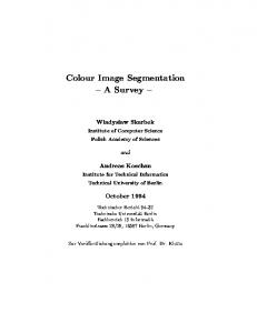
A new representation for color images have been developed. The method can be regarded as an extension to the existing BSP representation for grey scale image. The partitioning is done by thresholding the colour image in 3D space and a goodness of fit criterion is tested for all possible lines to decide the partitioning line. The proposed representation is used in image coding application. It was shown that it has a good potential in coding image better than JPEG at higher bit rate. A brief discussion on the possibility of using the representation in image indexing application have also been made. Acknowledgment The test images used in Fig 6 were obtained from MIT Media Lab web site. FIG 3. Coding of build1 image. From left to right and top to bottom wise: Original image (24 bpp), 1 st partition (4e-4 bpp), 2 nd (6e-4 bpp), 4th (2e-3 bpp), 8th (0.03 bpp), 10th (0.1 bpp), 12th (0.27 bpp), 16th (0.82 bpp) and 20th (1.3 bpp). For comparison purpose, JPEG compression standard is performed on the same image set and its result is plotted on the same rate distortion graphs which are shown in Fig 4. Although the graphs show that JPEG has a superior performance at low bit rate compression, BSP method has a good potential in high bit rate compression. As can be seen from the graphs that as the bit rate increases the distortion rapidly decreases for BSP method but only slightly for JPEG. The result of the two methods can also be inspected visually. In Fig 5 the original peppers image and the compressed image from both methods are shown. The size of all of the images is reduced to 77% to fit to the page. It is shown that the proposed method gives comparable result visually with JPEG.

4.2 Content Based Image Indexing Intuitively, similar images are partitioned in a similar way. For example images containing a horizon are most likely to be partitioned initially by a horizontal line. Furthermore, the top polygon usually represent the sky hence its color is sky blue while the bottom one is usually dark brown if it is earth, or green if grass or deep blue if it is a sea. Fig 6 shows how similar images are

6

REFERENCES

[1] M. de Berg, et al, Computational Geometry: Algorithms and Applications, Springer, 1997 [2] J.B. Fraleigh, A First Course in Abstract Algebra. Reading, MA: Addison-Wesley, 1982 [3] D.A. Huffman, "A Method for the Construction of Minimum Redudancy Codes", Proc. IRE, vol. 40, pp 1098-1101 [4] T.S. Lee "Image Representation using 2D Gabor Wavelets", IEEE Trans. Pattern Analysis. Machine Intelligence, vol. 18, pp.959-971, 1995 [5] S.C. Pei and C.M. Cheng, "Color image processing by using binary quaternion moment-preserving thresholding", IEEE Trans. on Image Processing, vol. 8, pp.614-628, 1999 [6] R.W. Picard, "Content Access for Image/Video Coding: "The Fourth Criterion"", MIT Media Lab Perceptual Computing Section Technical Report, No. 295, Statement for Panel on "Computer Vision and Image/Video Compression", ICPR94, Jerusalem [7] H. Radha, M. Vetterli, R. Leonardi, "Image compression using binary space partitioning tree", IEEE Trans. on Image Processing, vol.5, pp.1610-1624, 1996 [8] P.K. Sahoo, S. Soltani and A.K.C. Wong, "A survey of thresholding techniques", Computer Vision Graphic and Image Processing, pp. 233-260, 1988 [9] P. Salembier, L. Garrido, "Binary partition tree as an efficient representation for image processing, segmentation, and information retrieval", IEEE Trans. Image Processing, vol. 9, pp. 561-576, 2000 [10] A.J. Tabatabai and O.R. Mitchell, "Edge location to subpixel values in digital imagery", IEEE. Trans. Pattern

© International Conference on Color in Graphics and Image Processing - CGIP’2000

Analysis and Machine Intelligence, vol.6, pp. 188-201, 1984 [11] W.H. Tsai, "Moment preserving thresholding: A new approach", Computer Vision Graphic and Image Processing, pp. 377-393, 1985 [12] Y.P. Wang, "Image Representation using Multiscale Differential Operators", IEEE Trans. Image Processing, vol. 8, pp. 1757-1771, 1999

[13] C.K. Yang and W.H. Tsai, "Reduction of color space dimensionality by moment-preserving thresholding and its application for edge detection in color images", Pattern Recognition Letters, vol.17, pp.481-490, 1996

BSP

BSP

JPEG

JPEG

JPEG

BSP

BSP

BSP JPEG

BSP

JPEG

JPEG

FIG 4. Rate distortion graphs for the test images. Red lines are due to BSP coding and blue lines are due to JPEG compression standard.

FIG 4. The original images and their first three level of partitioned image (edge enhanced for better visualisation)

© International Conference on Color in Graphics and Image Processing - CGIP’2000

FIG 5: Compression result of peppers image. From left to right and top to bottom order. Original image (24 bpp), compressed image with BSP (1.4 bpp) and compressed image with JPEG (1.4 bpp)