Mar 12, 2013 - Professeur, Université Lille 1. Rapporteur ...... (Holland, 1975), memetic algorithms (Prins, 2004) and adaptive memory procedure (Rochat.
Column Generation for Bi-Objective Integer Linear Programs : Application to Bi-Objective Vehicle Routing Problems Boadu Mensah Sarpong
To cite this version: Boadu Mensah Sarpong. Column Generation for Bi-Objective Integer Linear Programs : Application to Bi-Objective Vehicle Routing Problems. Other [cs.OH]. Institut d’Optique Graduate School, 2013. English. .
HAL Id: tel-01078006 https://tel.archives-ouvertes.fr/tel-01078006 Submitted on 27 Oct 2014
HAL is a multi-disciplinary open access archive for the deposit and dissemination of scientific research documents, whether they are published or not. The documents may come from teaching and research institutions in France or abroad, or from public or private research centers.
L’archive ouverte pluridisciplinaire HAL, est destin´ee au d´epˆot et `a la diffusion de documents scientifiques de niveau recherche, publi´es ou non, ´emanant des ´etablissements d’enseignement et de recherche fran¸cais ou ´etrangers, des laboratoires publics ou priv´es.
` THESE En vue de l’obtention du
´ DE TOULOUSE DOCTORAT DE L’UNIVERSITE D´ elivr´ e par : l’Institut National des Sciences Appliqu´ees de Toulouse (INSA de Toulouse)
Pr´ esent´ ee et soutenue le 3/12/2013 par :
Boadu Mensah
Sarpong
Column Generation for Bi-Objective Integer Linear Programs : Application to Bi-Objective Vehicle Routing Problems
´ Ecole doctorale et sp´ ecialit´ e: EDSYS : Informatique 4200018 Unit´ e de Recherche : Laboratoire d’Analyse et d’Architecture des Syst`emes (LAAS-CNRS) Directeur(s) de Th` ese : Christian Artigues et Nicolas Jozefowiez
JURY : Dominique Feillet
Pr´esident du Jury
Daniel Vanderpooten
Professeur, Ecole des Mines de Saint-Etienne Professeur, Universit´e Paris Dauphine
¨ bbecke Marco Lu
Professeur, Univerisit´e RWTH Aachen
Rapporteur
Clarisse Dhaenens
Professeur, Universit´e Lille 1
Rapporteur
Christian Artigues
Directeur de Recherche, LAAS-CNRS, Toulouse Maˆıtre de Conf´erences, INSA de Toulouse
Nicolas Jozefowiez
Examinateur
Directeur de Th`ese Co-Directeur de Th`ese
Acknowledgements I would like to thank my two PhD directors Christian and Nicolas for proposing this thesis topic to me and teaching me how to do academic research the right way. They still believed and stood by me during difficult times when I was making no progress in my work. I’m also grateful to the referees and other members of my PhD defense jury for their corrections, comments, and insightful questions. Special thanks to Professor Tolga Bekta¸s of the University of Southamption who hosted me for a period of ten weeks during the summer of 2012. The short time I spent with him taught me so much academically and also in developing a better working habit. Thanks to all past and present members of the ROC group at LAAS-CNRS who provided me with a friendly environment for my research. I would finally want to thank my family, friends and loved ones who helped me in diverse ways all of which I cannot state here. I really appreciate your support.
ii
Abstract Multi-objective optimization deals with finding solutions to problems for which several objectives (or criteria) are considered. Unlike in single objective optimization, the optimal value of a multi-objective problem is a set of points called “the nondominated set”. Lower and upper bounds of a multi-objective problem can also be described using sets. For most practical problems, the variables considered in multi-objective optimization represent non fractionable items and thus we talk of multi-objective integer programs. In order to obtain good lower and upper bounds that can be used in the design of exact methods, some problems are usually formulated with an exponential number of decision variables and these problems are solved by column generation. The work of this thesis seeks to contribute to the study of the use of column generation in multi-objective integer linear programming. We do this by studying a bi-objective vehicle routing problem which may be seen as a generalization of several other vehicle routing problems. We propose mathematical formulations for this problem and also find ways to quickly compute lower bounds by column generation. Since the subproblems solved when computing lower bounds have similar structures, we propose intelligent ways of treating some of these subproblems simultaneously rather than independently. Keywords: Integer linear programming, column generation, multi-objective optimization, combinatorial optimization, vehicle routing
R´ esum´ e L’optimisation multi-objectif concerne la r´esolution de probl`emes pour lesquels plusieurs objectifs (ou crit`eres) contradictoires sont pris en compte. Contrairement aux probl`emes d’optimisation ayant un seul objectif, un probl`eme multi-objectif ne poss`ede pas une valeur optimale unique mais plutˆot un ensemble de points appel´es “ensemble non domin´e”. Les bornes inf´erieures et sup´erieures d’un probl`eme multi-objectif peuvent ˆetre ´egalement d´ecrites par des ensembles. Dans la pratique, les variables utilis´ees en optimisation multiobjectif repr´esentent souvent des objets non fractionnables et on parle alors de probl`emes multi-objectif en nombres entiers. Afin d’obtenir de meilleures bornes qui peuvent ˆetre utilis´ees dans la conception de m´ethodes exactes, certains probl`emes sont formul´es avec un nombre exponentiel de variables de d´ecision et ces probl`emes sont r´esolus par la m´ethode de g´en´eration de colonnes. Les travaux de cette th`ese visent `a contribuer `a l’´etude de l’utilisation de la g´en´eration de colonnes en programmation lin´eaires en nombres entiers multi-objectif. Pour cela nous ´etudions un probl`eme de tourn´ees de v´ehicules bi-objectif qui peut ˆetre consid´er´e comme une g´en´eralisation de plusieurs autres probl`emes de tourn´ees de v´ehicules. Nous proposons des formulations math´ematiques pour ce probl`eme et des techniques pour acc´el´erer le calcul des bornes inf´erieures par g´en´eration de colonnes. Les sous-probl`emes qui doivent ˆetre r´esolus pour le calcul des bornes inf´erieures ont une structure similaire. Nous exploitons cette caract´eristique pour traiter simultan´ement certains sous-probl`emes plutˆ ot qu’ind´ependamment. Mot-cl´ es: Programmation lin´eaire en nombres entiers, g´en´eration de colonnes, optimisation multi-objectif, optimisation combinatoire, tourn´ees de v´ehicules iii
Contents General Introduction Context . . . . . . . . . . . . . . . . . . . . . . . . . . . . . . . . . . . . . . . . . Organization and Contributions . . . . . . . . . . . . . . . . . . . . . . . . . . . . Notation . . . . . . . . . . . . . . . . . . . . . . . . . . . . . . . . . . . . . . . . . 1 Column Generation for Vehicle Routing Problems 1.1 Introduction . . . . . . . . . . . . . . . . . . . . . . . . . . . . . . . 1.2 Vehicle Routing Problems . . . . . . . . . . . . . . . . . . . . . . . 1.2.1 Formulations . . . . . . . . . . . . . . . . . . . . . . . . . . 1.2.2 Solution Methods . . . . . . . . . . . . . . . . . . . . . . . . 1.3 Column Generation . . . . . . . . . . . . . . . . . . . . . . . . . . . 1.3.1 Basic Definitions and Principles . . . . . . . . . . . . . . . . 1.3.2 Implementation and Other Issues . . . . . . . . . . . . . . . 1.4 The Elementary Shortest Path Problem with Resource Constraints 1.4.1 Overview of Solution Methods . . . . . . . . . . . . . . . . 1.4.2 The Decremental State Space Relaxation Algorithm . . . . 1.5 The Minimum-Maximum Distance-Constrained CVRP . . . . . . . 1.5.1 Problem Description . . . . . . . . . . . . . . . . . . . . . . 1.5.2 Master Problem and Subproblem . . . . . . . . . . . . . . . 1.5.3 Solving the Subproblem . . . . . . . . . . . . . . . . . . . . 1.5.4 Computational Experiments . . . . . . . . . . . . . . . . . . 1.6 Conclusion . . . . . . . . . . . . . . . . . . . . . . . . . . . . . . . 2 Multi-Objective Optimization 2.1 Introduction . . . . . . . . . . . . . . 2.2 Basic Definitions and Principles . . . 2.3 Solution Approaches . . . . . . . . . 2.3.1 A priori approaches . . . . . 2.3.2 Progressive approaches . . . . 2.3.3 A posteriori approaches . . . 2.4 Approaches for Managing Objectives 2.4.1 Scalar Approaches . . . . . . 2.4.2 Non-Scalar Approaches . . . 2.4.3 Pareto Approaches . . . . . . 2.4.4 Indicator-Based Approaches .
. . . . . . . . . . .
. . . . . . . . . . .
. . . . . . . . . . .
. . . . . . . . . . .
. . . . . . . . . . .
. . . . . . . . . . .
. . . . . . . . . . .
. . . . . . . . . . .
. . . . . . . . . . .
. . . . . . . . . . .
. . . . . . . . . . .
. . . . . . . . . . .
. . . . . . . . . . .
. . . . . . . . . . .
. . . . . . . . . . .
. . . . . . . . . . .
. . . . . . . . . . .
. . . . . . . . . . . . . . . . . . . . . . . . . . .
. . . . . . . . . . . . . . . . . . . . . . . . . . .
. . . . . . . . . . . . . . . . . . . . . . . . . . .
. . . . . . . . . . . . . . . . . . . . . . . . . . .
1 1 2 3
. . . . . . . . . . . . . . . .
5 5 5 7 9 10 11 14 15 16 17 19 19 20 21 24 27
. . . . . . . . . . .
29 29 30 32 33 34 34 34 34 36 37 37 v
2.5
2.6
2.7
Solution Methods . . . . . . . . . . . . . . . . . . . 2.5.1 Lower and Upper Bounds . . . . . . . . . . 2.5.2 Exact Methods . . . . . . . . . . . . . . . . 2.5.3 Approximation Methods . . . . . . . . . . . Evaluating Approximation Methods and Solutions 2.6.1 The Hypervolume Indicators . . . . . . . . 2.6.2 The Binary ε-Indicator . . . . . . . . . . . Conclusion . . . . . . . . . . . . . . . . . . . . . .
. . . . . . . .
. . . . . . . .
. . . . . . . .
. . . . . . . .
. . . . . . . .
. . . . . . . .
. . . . . . . .
. . . . . . . .
. . . . . . . .
3 Column Generation for Bi-Objective Integer Programs 3.1 Introduction . . . . . . . . . . . . . . . . . . . . . . . . . . . . . . . 3.2 Constructing Bound Sets for BOIPs . . . . . . . . . . . . . . . . . 3.2.1 Using the Weighted Sum Method . . . . . . . . . . . . . . . 3.2.2 Using the ε-Constraint Method . . . . . . . . . . . . . . . . 3.3 Constructing Lower Bound Sets for BOIPs by Column Generation 3.3.1 Column Search Strategies . . . . . . . . . . . . . . . . . . . 3.3.2 Column Generation for BOIPs with a Min-Max Objective . 3.3.3 Column Search Strategies for a BOIPMMO . . . . . . . . . 3.4 Evaluating the Quality of Bound Sets . . . . . . . . . . . . . . . . 3.4.1 Bound Sets for the Bi-Objective Set Covering Problem . . . 3.5 Conclusions . . . . . . . . . . . . . . . . . . . . . . . . . . . . . . . 4 The Bi-Objective Multi-Vehicle Covering Tour Problem 4.1 Introduction . . . . . . . . . . . . . . . . . . . . . . . . . . . 4.2 Description of the BOMCTP . . . . . . . . . . . . . . . . . 4.2.1 Cover Distance Induced by a Set of Routes . . . . . 4.3 Formulation 1 . . . . . . . . . . . . . . . . . . . . . . . . . . 4.3.1 Restricted LP Master Problem . . . . . . . . . . . . 4.3.2 Dual of LPM(ε) . . . . . . . . . . . . . . . . . . . . 4.3.3 Sub-problem corresponding to RLPM(ε) . . . . . . . 4.3.4 Solving S(ε) . . . . . . . . . . . . . . . . . . . . . . . 4.4 Formulation 2 . . . . . . . . . . . . . . . . . . . . . . . . . . 4.4.1 Restricted LP Master Problem . . . . . . . . . . . . 4.4.2 Dual of LPM(ε) . . . . . . . . . . . . . . . . . . . . 4.4.3 Subproblem corresponding to RLPM(ε) . . . . . . . 4.4.4 Solving S(ε) . . . . . . . . . . . . . . . . . . . . . . . 4.4.5 Implementation of Column Search Strategies . . . . 4.5 Computational Results . . . . . . . . . . . . . . . . . . . . . 4.5.1 Description of Instances and Experiments . . . . . . 4.5.2 Summary of Results for Formulation 1 . . . . . . . . 4.5.3 Summary of Results for Formulation 2 . . . . . . . . 4.5.4 Comparison of Formulations 1 and 2 . . . . . . . . . 4.6 Conclusion . . . . . . . . . . . . . . . . . . . . . . . . . . . vi
. . . . . . . . . . . . . . . . . . . .
. . . . . . . . . . . . . . . . . . . .
. . . . . . . . . . . . . . . . . . . .
. . . . . . . . . . . . . . . . . . . .
. . . . . . . . . . . . . . . . . . . . . . . . . . . . . . . . . . . . . . .
. . . . . . . . . . . . . . . . . . . . . . . . . . . . . . . . . . . . . . .
. . . . . . . . . . . . . . . . . . . . . . . . . . . . . . . . . . . . . . .
. . . . . . . . . . . . . . . . . . . . . . . . . . . . . . . . . . . . . . .
. . . . . . . .
38 38 39 44 45 46 46 48
. . . . . . . . . . .
49 49 51 52 53 55 56 66 68 71 73 74
. . . . . . . . . . . . . . . . . . . .
75 75 77 77 78 79 79 80 80 81 82 82 82 83 84 88 88 88 89 94 97
Conclusions and Perspectives 99 Conclusions . . . . . . . . . . . . . . . . . . . . . . . . . . . . . . . . . . . . . . . 99 Perspectives . . . . . . . . . . . . . . . . . . . . . . . . . . . . . . . . . . . . . . . 100 A R´ esum´ e´ etendu 103 A.1 Introduction . . . . . . . . . . . . . . . . . . . . . . . . . . . . . . . . . . . . 103 A.1.1 Principe de G´en´eration de Colonnes . . . . . . . . . . . . . . . . . . 103 A.1.2 Optimisation Multi-Objectif . . . . . . . . . . . . . . . . . . . . . . . 104 A.1.3 Contributions . . . . . . . . . . . . . . . . . . . . . . . . . . . . . . . 104 A.2 G´en´eration de Colonnes pour les Probl`emes Lin´eaires en Nombres Entiers Bi-Objectif . . . . . . . . . . . . . . . . . . . . . . . . . . . . . . . . . . . . 105 A.2.1 Construction de Bornes Inf´erieures . . . . . . . . . . . . . . . . . . . 105 A.2.2 Construction de Bornes Inf´erieures par G´en´eration de Colonnes . . . 106 A.2.3 Un Algorithme G´en´eralis´e de G´en´eration de Colonnes Pour les Probl`emes Lin´eaires en Nombres Entiers Bi-Objectif . . . . . . . . . 108 A.2.4 G´en´eration de Colonnes pour les PLNE Bi-Objectif ayant une Fonction Objectif Min-Max . . . . . . . . . . . . . . . . . . . . . . . . . . 110 A.3 Probl`eme de Tourn´ee Couvrante Bi-Objectif `a Plusieurs V´ehicules . . . . . 111 A.3.1 Description du Probl`eme . . . . . . . . . . . . . . . . . . . . . . . . 111 A.3.2 Formulation 1 . . . . . . . . . . . . . . . . . . . . . . . . . . . . . . . 111 A.3.3 Formulation 2 . . . . . . . . . . . . . . . . . . . . . . . . . . . . . . . 112 A.4 R´esultats des exp´eriences . . . . . . . . . . . . . . . . . . . . . . . . . . . . 114 A.4.1 Comparison de Deux M´ethodes de Scalarisation . . . . . . . . . . . . 115 A.4.2 R´esultats pour PTCBOP . . . . . . . . . . . . . . . . . . . . . . . . 116 A.5 Conclusions et Perspectives . . . . . . . . . . . . . . . . . . . . . . . . . . . 119 Bibliography
120
vii
List of Algorithms 1.1 1.2 2.1 2.2 3.1 3.2 3.3 3.4 3.5 3.6 3.7 3.8 3.9
A Column Generation Algorithm . . . . . . . . . . . . . . . DSSR - The Decremental State Space Relaxation Algorithm Aneja and Nair (1979)’s Method. . . . . . . . . . . . . . . . An Exact ε-Constraint Method for BOCO problems . . . . Using an ε-constraint method to compute a lower bound set A generalized column generation method for BOIPs . . . . k-Step Point-by-Point Search (k-PPS) . . . . . . . . . . . . Generate a set of Points (weighted sum method) . . . . . . Generate a set of Points (ε-constraint method) . . . . . . . Sequential Search 1 . . . . . . . . . . . . . . . . . . . . . . . Sequential Search 2 . . . . . . . . . . . . . . . . . . . . . . . Improved Point-by-Point Search (IPPS) . . . . . . . . . . . Solve-Once-Generate-for-All (SOGA) . . . . . . . . . . . . .
. . . . . . . . . . . . .
. . . . . . . . . . . . .
. . . . . . . . . . . . .
. . . . . . . . . . . . .
. . . . . . . . . . . . .
. . . . . . . . . . . . .
. . . . . . . . . . . . .
. . . . . . . . . . . . .
. . . . . . . . . . . . .
12 18 41 43 54 57 59 62 63 63 64 69 70
ix
List of Figures 1.1 1.2 1.3 1.4
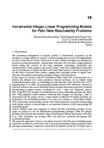
The basic variants of vehicle routing problems and their interconnections Interactions between LPM, RLPM, DLPM and DRLPM. . . . . . . . . . Some convergence related issues of a column generation method. . . . . . Dominance rules for modeling exact resource consumption. . . . . . . . .
. 6 . 13 . 15 . 22
2.1 2.2 2.3 2.4 2.5 2.6 2.7 2.8 2.9 2.10 2.11 2.12 2.13
Pareto dominance between solutions. . . . . . . . . . . . . . . . . . Common shapes of the tradeoff surface for a bi-objective problem. Two qualities of approximations. . . . . . . . . . . . . . . . . . . . Solutions found by a weighted sum method for λ1 = λ2 = 0.5. . . . Solutions found by the ε-constraint method. . . . . . . . . . . . . . Solutions found by the lexicographic method. . . . . . . . . . . . . Bounds for a BOCO problem. . . . . . . . . . . . . . . . . . . . . . Different stages of the two phases method. . . . . . . . . . . . . . . Illustration of Sylva and Crema’s Method with λ1 = λ2 = 0.5. . . . Illustration of the parallel partitioning method. . . . . . . . . . . . Difficulty in comparing approximation solution sets. . . . . . . . . The hypervolume indicators. . . . . . . . . . . . . . . . . . . . . . The Binary ε-indicator. . . . . . . . . . . . . . . . . . . . . . . . .
. . . . . . . . . . . . .
3.1 3.2 3.3 3.4
3.6 3.7
Constructing a lower bound set through a weighted sum method. . . . . . Constructing a lower bound set through an ε-constraint method. . . . . . Order in which points of a lower bound set are identified by the PPS. . . Possible order in which points of a lower bound set are identified by the k-PPS. . . . . . . . . . . . . . . . . . . . . . . . . . . . . . . . . . . . . . . Possible order in which points of a lower bound set are identified by a sequential search approach. . . . . . . . . . . . . . . . . . . . . . . . . . . Calculation of quality measures in the case of a weighted sum method. . . Calculation of quality measures in the case of an ε-constraint method. . .
. 65 . 72 . 72
4.1 4.2 4.3 4.4 4.5 4.6
An example of a solution to the CTP . . . . . An example of a solution to the MCTP . . . The cover distance induced by a set of routes. Non-additive nature of subproblem. . . . . . . Dominance relationship between labels. . . . IPPS heuristic for the BOMCTP. . . . . . . .
. . . . . .
3.5
. . . . . .
. . . . . .
. . . . . .
. . . . . .
. . . . . .
. . . . . .
. . . . . .
. . . . . .
. . . . . .
. . . . . .
. . . . . .
. . . . . .
. . . . . . . . . . . . .
. . . . . .
. . . . . . . . . . . . .
. . . . . .
. . . . . . . . . . . . .
. . . . . .
. . . . . . . . . . . . .
. . . . . .
31 32 33 35 36 38 40 42 44 45 46 47 47
. 53 . 54 . 58 . 60
75 76 78 83 85 86 xi
xii
4.7 4.8
SOGA heuristic for the BOMCTP. . . . . . . . . . . . . . . . . . . . . . . . 87 Ideas for defining more general lower bound sets. . . . . . . . . . . . . . . . 101
A.1 A.2 A.3 A.4 A.5 A.6 A.7 A.8
Construction d’une borne inf´erieure par ε-contrainte. Un algorithme g´en´eralis´e de g´en´eration de colonnes. Heuristique IPPS pour PTCBOP. . . . . . . . . . . . Heuristique SOGA pour PTCBOP. . . . . . . . . . . Calculation des m´etriques d’´evaluation . . . . . . . . Formulation 1 : Temps d’ex´ecutions . . . . . . . . . Formulation 2 : Temps d’ex´ecutions . . . . . . . . . Bornes pour une instance de type |T | = 1, |V | = 50, q = ∞. . . . . . . . . . . . . . . . . . . . . . . . . . .
. . . . . . . . . . . . . . . . . . . . . . . . . . . . . . . . . . . . . . . . . . . . . . . . . . . . . . . . . . . . . . . . . . . . . . . . . . . . . . . . . . . . |W | = 150, p = 5, et . . . . . . . . . . . .
. . . . . . .
106 108 114 115 116 117 118
. 118
List of Tables 1.1 1.2
Comparison between Gamache et al’s and New Dominance Relations . . . . 25 Performance of Relaxations . . . . . . . . . . . . . . . . . . . . . . . . . . . 26
3.1
Comparison of lower bound sets for the BOSCP . . . . . . . . . . . . . . . . 74
4.1 4.2 4.3 4.4 4.5 4.6
Quality of bound sets for Formulation 1 . . . . . . . . . . . Computational times for Formulation 1 . . . . . . . . . . . Quality of bound sets for Formulation 2 . . . . . . . . . . . Computational times for Formulation 2 . . . . . . . . . . . Comparison of Formulations 1 and 2 . . . . . . . . . . . . . Comparison of Lower Bound Sets for Formulations 1 and 2
. . . . . .
. . . . . .
. . . . . .
. . . . . .
. . . . . .
. . . . . .
. . . . . .
. . . . . .
. . . . . .
90 91 92 93 95 96
xiii
General Introduction Context Many optimization problems encountered in practical applications concern two or more contradictory objectives (or criteria). These problems, called multi-objective optimization problems, are different from classical optimization problems in the sense that the optimal value of a multi-objective problem is a set of points (called ”the nondominated set”) rather than a unique optimal value. No member of the nondominated set is better than another member over all the objective funcions. Lower and upper bounds of a MOP can also be described using sets. For most practical problems, the variables considered in MOPs represent non fractionable items (eg. number of persons) and thus we talk of multi-objective integer programs (MOIP). MOIP are solved mainly by heuristics and metaheuristics and although these methods are effective, they provide no guarantee of finding the exact nondominated set. Few exact methods have been proposed in the literature for MOIPs having two objectives. Most exact methods for solving optimization problems work by computing a lower bound and an upper bound so that the optimal value of the problem lies between these two values. The quality of these bounds are improved until they are equal (in which case we have the exact optimal value) or until the gap between them becomes reasonably small (in this case, we have a good approximation for the optimal solution together with a measure of quality for the approximation). Due to the role that lower and upper bounds play in solving optimization problems, there is the need to develop good mathematical models and efficient ways of computing such bounds for multi-objective problems. In the single objective case, a popular way of computing good lower and upper bounds for some classes of integer programs (eg. vehicle routing problems) is by formulating them with an exponential number of variables. It is impractical and sometimes impossible to explicitly list all of the variables (or columns) involved in such formulations and so they are solved by column generation methods. Column generation is an iterative method and the main idea of the method is to decompose an original problem into two main parts namely a restricted master problem and a subproblem. The restricted master problem is a copy of the original problem in which only a few of the variables are kept. The role of the subproblem is to propose new variables to be introduced into the master problem in order to prove the convergence of the method or possibly improve the current optimal value. An iteration of column generation involves solving the linear relaxation of the master problem and then solving the subproblem to verify if it will propose some new variables (through a pricing process) to be added to the master problem. This iterative process ends when the 1
subproblem proposes no new variables. Although designed for non-integer linear problems, column generation has been a very successful method for solving integer linear programs when it is integrated in a branch-and-bound framework yielding a branch-and-price scheme. In spite of the importance of column generation, only a few published papers deal with its application to multi-objective problems. The objective of this thesis is to contribute to the study of column generation as applied to multi-objective integer linear programs. We do this through the study of a bi-objective vehicle routing problem. We seek to propose good mathematical formulations for this problem and also find ways of computing good lower bounds by column generation. More precisely, subproblems having similar structures need to be solved when computing lower bound so we seek to propose intelligent ways of treating some of these subproblems simultaneously rather than idependently.
Organization and Contributions The manuscript is organized into four main chapters. Chapter 1 gives an overview of column generation as applied to single objective vehicle routing problems and our contribution on an original variant. After introducing the different terminologies and formulations for vehicle routing problems, the basic definitions and principles of column generation are discussed. Next, we discuss the different stages of solving the very basic variant of the vehicle routing problem by column generation. A section in this chapter discusses the elementary shortest path problem with resource constraints. Indeed, this problem appears as a subproblem when solving several variants of the vehicle routing problem by a column generation method. In the last section of this chapter, we present an original variant of the vehicle routing problem and a way to solve it by a column generation method. The main interest of this problem stems from the subproblem we encounter. We propose a new dominance relation when solving the subproblem by a dynamic programming algorithm. In Chapter 2 we give a review of multi-objective optimization. We discuss the interest of multi-objective optimization problems, the different approaches used in managing the multiple objectives, as well as different solution approaches. In particular, we review some popular exact methods for bi-objective integer programs. We also present some quality measures used in evaluating approximation methods and the approximate solutions they produce. Chapter 3 discusses how good lower and upper bounds can be computed for bi-objective integer linear programs. The principle is to use sets of points having certain properties in the definition of lower and upper bounds. We therefore refer to lower and upper bound sets. We propose a generic column generation algorithm for computing a lower bound set for a problem when it is formulated with an exponential number of columns. The main idea used is to first convert the bi-objective program into single objective through a scalarization method. We then solve linear relaxations of the resulting single objective problem several times by varying the necessary parameters. We show that regardless of the scalarization method used, the subproblems that need to be solved when computing the members of a lower bound set have similar structures. Due to this, we propose different strategies to take advantage of the similar subproblem structures. In order to test the different ideas presented in Chapter 3, an application problem is presented in Chapter 4. The problem is a generalization of the covering tour problem 2
namely the bi-objective multi-vehicle covering tour problem. Two different formulations are presented for this problem and different column generation approaches adapted to each formulation are tested. Summary of the experiments performed and discussion of the results obtained are presented at the end of the chapter. The results show the quality of the proposed formulations and the interest of the intelligent column generation techniques designed in Chapter 3 on this problem. The manuscript ends with some general concluding remarks as well as future research directions in the short term, middle term, and long term.
Notation Throughout this manuscript, we will usually need to compare vectors of real numbers. In general, there is no canonical way of doing this and so we need to clarify the notations used. Given a positive integer n ≥ 2 and any two arbitrary vectors of real numbers x, y ∈ Rn , we will use the following notation : • x = y if xi = yi for i = 1, . . . , n , • x < y if xi < yi for i = 1, . . . , n , • x 5 y if xi ≤ yi for i = 1, . . . , n , • x ≤ y if x 5 y but x 6= y . We will also write : • Rn> for {x ∈ Rn : x > 0} , • Rn≥ for {x ∈ Rn : x ≥ 0} , • Rn= for {x ∈ Rn : x = 0} .
3
Chapter 1
Column Generation for Vehicle Routing Problems 1.1
Introduction
In this chapter, we discuss the application of column generation to vehicle routing problems (VRPs). In Section 1.2, we present terminologies for VRPs as well as the different formulations proposed in the literature. We also give an overview of some general methods used in solving VRPs. Section 1.3 follows with a discussion on column generation as applied to VRPs by using the basic variant of the VRP (the capacitated VRP or CVRP) as an example. The elementary shortest path problem with resources constraints (ESPPRC) which usually appears as a subproblem in vehicle routing problems solved by column generation is discussed in Section 1.4. We present a specific vehicle routing problem and discuss its solution by column generation in Section 1.5. The interest of this problem stems from the fact that the subproblem encountered presents a challenge to dynamic programming algorithms used in its solution. We propose some ideas that can be used to overcome this challenge. Section 1.6 ends the chapter with some concluding remarks. Related Publications. The ideas presented in Section 1.5 is the core of an article which is currently under prepartion for submission to an international journal. These ideas were developed following a 10 week research visit to the University of Southampton in the United Kingdom. The research was performed at the Centre for Operational Research, Management Sciences and Information Systems (http://www.southampton.ac.uk/cormsis/). During this stay, the author worked under the supervision of Professor Tolga Bekta¸s at the School of Management Sciences (http://www.southampton.ac.uk/management/about/staff/ tb12v07.page#background).
1.2
Vehicle Routing Problems
Vehicle Routing Problems (VRP) are concerned with the optimal routing of a fleet of vehicles from one or several depots in order to deliver services to a number of geographically scattered customers. The first of such problems was presented by Dantzig and Ramser 5
(1959). Their problem was to design optimal routes to deliver gasoline from a bulk terminal to a large number of service stations. Since that time, several variants of VRP have been proposed to address problems encountered in real-world transportation systems. The different variants stems from the different kind of services that may be offered as well as the different operational constraints that need to be respected. In general, two main types of services namely delivery and collection are provided. Numerous operational constraints appear in real applications. Some of the most common ones are limits on the capacity of a vehicle, maximum limits placed on the length of a route, specific periods during which a customer may be visited, an order in which customers may be visited and the type of service that may be provided for each customer (only delivery, only collection, both delivery and collection). In the very basic version of the VRP (the capacitated VRP or CVRP), the main operational constraint is that the total amount of goods delivered by a single vehicle cannot exceed a fixed capacity. If in addition to delivering goods, the vehicle may also collect goods from the customers they visit, then we talk of the VRP with pick up and delivery (VRPPD). Other basic variants of the CVRP are the distance-constrained capacitated VRP (DCVRP) in which a maximum limit is placed on the length of each route, the VRP with time windows (VRPTW) in which each customer should be visited within a specific time period, and the VRP with backhauling (VRPB) in which for each customer a visiting vehicle either deliver goods, or collect goods, but not both. A representation of the interconnections between the basic variants of the VRP is given in Figure 1.1. Most times, we refer to the CVRP as the classical VRP because of the central role it plays in the classification of VRPs. Indeed, many algorithms developed for the CVRP can be adapted to take into account other complicated operational constraints Laporte (2007). The variants of VRP studied in recent times combine several of the constraints stated above and several other ones. VRP
Capacity
CVRP
g
lin au
h ack
B
VRPB
Time Windows
Route Length
Mi
xe
dS
erv
ice
VRPTW
VRPBTW
DCVRP
VRPPD
VRPPDTW
Figure 1.1: The basic variants of vehicle routing problems and their interconnections (Toth and Vigo, 2002). 6
The solution of a VRP is a set of routes (one for each vehicle) each of which starts and ends at a depot such that the demands (or requests) of all customers are satisfied and the global cost of transportation is minimised while respecting all operational constraints. The global cost of transportation may be measured based on different criteria such as the travel distance and/or time, and other costs linked to the use of a vehicle. The VRP is an NP-hard problem since it lies at the junction of two NP-hard problems namely the Bin Packing Problem (BPP) and the Traveling Salesman Problem (TSP). For each vehicle (or route), we need to determine the customers it will visit (BPP) and also give an order in which they are visited (TSP). Sometimes, measuring the cost of a route is a difficult problem in itself. Applications of VRPs exist in the domains of solid waste collection, street cleaning, school bus routing, dial-a-ride systems, transportation of handicapped persons, routing of salespeople, and maintenance of units (Toth and Vigo, 2002). Others are in the delivery of newspapers to retailers, of food and beverages to grocery stores and in the collection of milk products from dairy farmers (Golden et al., 2002). A general survey on VRPs can be found in Toth and Vigo (2002).
1.2.1
Formulations
There are three main types of model for VRPs found in the literature Toth and Vigo (2002). These are vehicle flow formulations, commodity flow formulations and set partitioning formulations. We may also differentiate between two-index and three-index flow formulations. We demonstrate the principles of vehicle flow formulations and set partitioning formulations by using the CVRP as an example. Most solution methods are based on one of these two. Only very few methods presented in the literature are based on commodity flow formulations. For this reason, commodity flow formulations are not discussed in this section. Let G = (V, A) be a complete graph where V = {v0 , . . . , vn } is a set of nodes and A = {(vi , vj ) : vi , vj ∈ V and i 6= j} is a set of arcs. Node v0 is the depot where all routes must start and also end whereas nodes v1 , . . . , vn represent n customer locations. A non-negative cost matrix D = (dij ) which satisfies the triangle inequality is defined on set A. Each customer has a fixed demand of qi which must fully be satisfied by a route that visits it. Let m be the total number of available vehicles. The CVRP consists in designing a set of at most m routes with total minimum cost such that each customer is visited by exactly one route and the sum of the demands of customers visited by a single route does not exceed the vehicle capacity, Q.
Vehicle Flow Formulations In this type of formulation, a binary variable xij is used to indicate whether the arc (vi , vj ) is used by a vehicle in the optimal solution (xij = 1), or not (xij = 0). Let ui be the load of 7
a vehicle after visiting customer vi . A vehicle flow formulation for the CVRP is given by : Minimize
X
(1.1)
dij xij
(vi ,vj )∈E
subject to:
X
x0j ≤ m ,
(1.2)
xi0 = 0 ,
(1.3)
(v0 ,vj )∈A
X
x0j −
(v0 ,vj )∈A
X (vi ,v0 )∈A
xij = 1
(vj ∈ V \{v0 }) ,
(1.4)
xij = 1
(vi ∈ V \{v0 }) ,
(1.5)
(vi , vj ∈ V \{v0 }, i 6= j) ,
(1.6)
qi ≤ σ i ≤ Q
(vi ∈ V \{v0 }) ,
(1.7)
σi ≥ 0
(vi ∈ V \{v0 }) ,
(1.8)
(vi , vj ∈ V ) .
(1.9)
X vi ∈V
X vj ∈V
σi + qj − σj + Qxij ≤ Q
xij ∈ {0, 1}
The objective of minimizing the total cost of the routes is given in (1.1). Constraint (1.2) limits the number of arcs that leaves the depot whereas (1.3) ensures that the number of arcs that enter the depot is the same as the number of those that leave it. Together, these two constraints ensure that not more than m routes are constructed. The indegree and outdegree constraints given by (1.4) and (1.5) respectively ensure that exactly one arc leaves and enter each customer node. Constraints (1.6) and (1.7) are subtour elimination constraints which were originally proposed for the TSP by Miller et al. (1960). These constraints eliminate routes that are not connected to the depot and also enforce the maximum capacity limits of vehicles. The domain of definition for the variables in σ and x are given by Constraints (1.8) and (1.9), respectively. Vehicle flow formulations are perhaps the most used type of formulation for VRPs. They are most suited for cases where the cost of a route can be expressed as the sum of the costs of the edges it uses. They can, however, not be used for cases where the cost of a route depends not just on the individual edges it uses but rather on the total sequence of the edges. Set Partitioning Formulations A set partitioning formulation for a VRP uses an exponential number of variables each of which is associated to a feasible route. A route is said to be feasible if it satisfies all operational constraints. For the CVRP, a feasible route is simply a Hamiltonian cycle that connects the depot to a subset of customer nodes in such a way that the sum of the demands of customers on the cycle does not exceed the capacity of the vehicle. This type of model for the VRP was first proposed by Balinski and Quandt (1964). Let Ω be the set of all feasible routes. Each feasible route k ∈ Ω has an associated cost ck which is given by the cost of the arcs it uses. For each customer node vi , we define a binary variable aik which takes a value of 1 if route k visits node vi and aik = 0 if this is 8
not the case. A binary variable θk is defined for each route k ∈ Ω to determine if the route is selected in the optimal solution (θk = 1) or not (θk = 0). A set-partitioning formulation for the CVRP is given by : Minimize
X
(1.10)
ck θk
k∈Ω
subject to :
X
(1.11)
θk ≤ m ,
k∈Ω
X
aik θk = 1
(vi ∈ V \{v0 }) ,
(1.12)
(k ∈ Ω) .
(1.13)
k∈Ω
θk ∈ {0, 1}
The solution of this formulation is a subset of feasible routes in Ω that minimizes the objective function (1.10) while ensuring that each customer node is visited by exactly one selected route (1.12). The cardinality of the subset must not exceed m as specified by Constraint (1.11). If m is reasonably large (eg. m ≥ n − 1), then this constraint may be dropped. The above formulation is very general and can easily take into account several other operational constraints on a single route. We only need to redefine what a feasible route represents in such situations. Since we assume that the cost matrix D satisfies the triangle inequality, we can transform the above set partitioning formulation into a set covering formulation by replacing (1.12) with X aik θk ≥ 1 (vi ∈ V \{v0 }) . (1.14) k∈Ω
The optimal objective value of both the set partitioning and the set covering models are the same. Indeed, if the optimal solution of a set covering model contains two or more routes that visit the same customer then this customer may be kept in just one of these routes and removed from all the rest. The resulting solution will still be feasible, and thanks to the triangle inequality, the new objective value will be less than or equal to that of the previous solution. One main advantage of using a set covering formulation instead of a set partitioning formulation is that the dual space in a set covering formulation is much smaller since the dual variables associated to Constraints 1.14 are restricted to only nonnegative values. This means that methods that rely heavily on these dual variables becomes much faster. A general disadvantage of both set partitioning and set covering models is that, the number of decision variables is huge. For example, in a simple instance of a CVRP with n = 15 we have about 15!/2 = 653, 837, 184, 000 routes (decision variables). It is, thus, impractical to list all of these variables and so methods that dynamically introduce the variables like column generation (discussed in Section 1.3) are employed.
1.2.2
Solution Methods
The Vehicle Routing Problem is one of the most studied combinatorial optimization problems. Different solution approaches ranging from exact methods, heuristics and metaheuristics have been proposed to tackle the numerous variants of the problem. Due to the difficulty of VRPs, most research effort concentrate on heuristics and metaheuristics 9
rather than on exact methods (Laporte, 2007). This is also probably because it is easier to adapt these methods to different variants. The main exact approaches for VRPs rely on relaxations and implicit enumeration techniques like branch-and-bound. Some of the most popular exact algorithms are branchand-cut in which cutting planes are combined with branch-and-bound, branch-and-price in which column generation is incorporated in a branch-and-bound framework, and Lagrangian relaxation. Among these, branch-and-cut algorithms are the most popular. Reviews on exact methods can be found in Laporte and Nobert (1987); Toth and Vigo (1998). As already indicated, the literature on heuristics and metaheuristics for VRPs is enormous. We only list just a few of them here. Dantzig and Ramser (1959) proposed the first heuristic approach when they introduced the VRP. A greedy heuristic namely the savings algorithm was later proposed by Clarke and Wright (1964) and this has gone on to become a very popular heuristic. The popularity of the savings algorithms is not due to its accuracy but rather its speed and the simplicity in implementing it (Laporte, 2007). Different types of metaheuristics have also been proposed to solve the CVRP and its variants. Examples are, local search algorithms like record-to-record travel (Dueck, 1993), tabu search (Glover, 1986), variable neighbourhood search (Mladenovi´c and Hansen, 1997), very large neighbourhood search (Ergun, 2001) and adaptive large neighbourhood search (Pisinger and Ropke, 2007). Some population search metaheuristics are genetic algorithms (Holland, 1975), memetic algorithms (Prins, 2004) and adaptive memory procedure (Rochat and Taillard, 1995). Other metaheuristics are learning mechanisms like neural networks and ant colony optimization (Schumann and Retzko, 1995; Ghaziri, 1991). Cordeau et al. (2005) presents a survey on metaheuristics for VRPs.
1.3
Column Generation
The birth of column generation traces back to the early 1960’s (Dantzig and Wolfe, 1960; Gilmore and Gomory, 1961, 1963) with its first applications to VRPs appearing some years afterwards (Appelgren, 1969, 1971). Its role in integer programming is to compute dual bounds (i.e. lower bounds for minimization problems and upper bounds for maximization problems). In order to ensure the integrality of solutions, it may be necessary to embed column generation in a branch-and-bound framework. We thus obtain the solution approach called branch-and-price. In this section, we will concentrate mainly on computing lower bounds of VRPs by column generation. A complete discussion of column generation and branch-and-price can be found in Barnhart et al. (1998) or in a recent book on the subject (Desaulniers et al., 2005). A very good paper that describes the application of column generation to VRPs is Feillet (2010). Lets consider the set covering model described by (1.10), (1.11), (1.13) and (1.14). Its 10
linear programming (LP) relaxation is given by : Minimize
X
(1.15)
ck θk
k∈Ω
subject to :
X
(1.16)
θk ≤ m ,
k∈Ω
X
aik θk ≥ 1
(vi ∈ V \{v0 }) ,
(1.17)
(k ∈ Ω) .
(1.18)
k∈Ω
θk ≥ Âă 0
Note: In the above formulating, we consider the variables in θk as being integers instead of binary in order avoid constraints of the form θk ≤ 1 in the dual formulation. It is clear, however, that this does not change the optimal value since any solution with θk ≥ 2 for a given k ∈ Ω will not be optimal. Let π0 be the non-positive dual variable associated with Constraint (1.16) and πi for vi ∈ V \{v0 } be non-negative dual variables associated with Constraints (1.17). The dual formulation of the relaxed set covering model is Maximize mπ0 +
X
(1.19)
πi
vi ∈V \{v0 }
subject to :
π0 +
X
aik πi ≤ ck
(k ∈ Ω) ,
(1.20)
vi ∈V \{v0 }
π0 ≤ 0 , πi ≥ 0
(1.21) (vi ∈ V \{v0 }) .
(1.22)
Suppose that the set of feasible routes Ω is manageable in the sense that all of its members can easily be listed and the resulting formulation can also be easily solved. Solving formulation (1.15 – 1.18) by the simplex algorithm requires that in each iteration, a non-basic variable with negative reduced cost is priced-out and enter the basis. The reduced cost of variable θk is defined as c˜k = ck − π0∗ −
X
aik πi∗ ,
(1.23)
vi ∈V \{v0 }
where π0∗ and πi∗ for vi ∈ V \{v0 } are optimal dual values at the current iteration. In selecting a non-basic variable to enter the basis, the simplex algorithm computes the reduced cost of all the non basic variables and picks the one having the most negative value. We call this technique explicit pricing and it is viable only when the set Ω is manageable. For problems in which there is a huge number of variables, explicit pricing becomes computationaly expensive and so we resort to a column generation method.
1.3.1
Basic Definitions and Principles
In column generation terminology, we refer to formulation (1.10), (1.11), (1.13) and (1.14) as the integer programming master problem (IPM) and its linear programming relaxation 11
given in (1.15 – 1.18) is called the linear programming master problem (LPM). We denote the dual formulation of LPM detailed in (1.19 – 1.22) as DLPM. The basic principle of column generation mimics the simplex algorithm but with two main differences. Firstly, since it is impractical to explicitly list all the members of Ω, we work with a reasonably small subset Ω1 ⊆ Ω for which LPM is primal feasible. The restriction of LPM to a subset Ω1 ⊆ Ω is called a restricted linear programming master problem (RLPM). Secondly, pricing of non-basic variables is now done implicitly by solving an auxilliary problem called the subproblem (SP). The subproblem is given by : minimize ck − π0∗ −
X
aik πi∗
subject to
k ∈ Ω\Ω1 .
(1.24)
vi ∈V \{v0 }
The Algorithm The algorithm starts by formulating a RLPM. At each iteration, the RLPM is first solved to obtained an optimal solution and a corresponding vector of dual values. Next, the subproblem is solved to see if any non-basic variables can be priced out in order to improve the current objective value. If the optimal value of the subproblem is non-negative then the current objective value of RLPM can not be improved and so an optimal solution of LPM has been found. If this is not the case then one or more columns having negative reduced costs are introduced into the RLPM and the process continues. Algorithm 1.1 summarizes a column generation method. Algorithm 1.1 A Column Generation Algorithm 1: Generate an initial set of columns Ω1 and formulate RLPM. 2: repeat 3: Solve RLPM(Ω1 ). 4: Solve subproblem and let Λ be the set of columns found. 5: Set Ω1 ← Ω1 ∪ Λ. 6: until Λ = ∅.
Primal and Dual Bounds We remind ourselves that column generation works on a RLPM but not directly on LPM since the size of Ω is very large. Given that a RLPM is obtained by depriving the LPM of some of its variables, every feasible solution of RLPM is also a feasible for LPM and hence an upper bound on LPM. The situation is however different in the dual space. Removing some variables from LPM (to formulate RLPM) corresponds to removing some constraints from DLPM. As a result, a feasible (even an optimal) solution for DRLPM may not be feasible for DLPM. Thus if the algorithm starts with a feasible RLPM then LPM remains primal feasible throughout the whole process but its dual feasibility is proved only at convergence. Let z¯ denote the optimal objective value of RLPM. If we have an upper bound ∗ κ on the optimal objective value zLP M of LPM then a lower bound may also be computed at each iteration of the algorithm. Let c˜∗ be the optimal solution of the subproblem, then 12
the following inequality holds ∗ z¯ + κ˜ c∗ ≤ zLP ¯. M ≤ z
(1.25)
This means that the algorithm may be stopped earlier before it converges since it is possible to verify the solution quality at any given time. Validity and Convergence of the Algorithm The validity and convergence of column generation relies on the following simple property of the models involved (see Figure 1.2). • The feasible space of RLPM is a subspace of the feasible space of LPM whereas the feasible space of DLPM is a subspace of that of DRLPM. This means that any feasible solution for RLPM is also a feasible for LPM and the corresponding objective value is an upper bound on the optimal value of LPM. Also, the feasible space of DLPM is a relaxation of the feasible space of DRLPM and so not all feasible solutions of DRLPM are feasible for DLPM. The optimal value of DRLPM, however, provides a lower bound on the optimal value of DLPM. In addition, if the optimal solution of DRLPM is feasible for DLPM, then it is also the optimal value of DLPM. Introducing new variables (or columns) in the RLPM corresponds to adding constraints to the DRLPM. Given that there is a finite number of elements in Ω, the algorithm converges after a finite number of iterations and so it is an exact method for the LPM. The hope is that the LPM will become both primal and dual feasible after introducing a reasonable small number of columns. In worse case, however, the method will only converge after all feasible columns have been added. DRLPM LPM
DLPM
RLPM
Figure 1.2: Interactions between LPM, RLPM, DLPM and DRLPM. Notes: RLPM is a subspace of LPM and so the optimal value of RLPM is an upper bound on the optimal value on LPM. On the other hand, DLPM is a subspace of DRLPM and so the optimal value of DRLPM is a lower bound on the optimal value of DLPM.
13
1.3.2
Implementation and Other Issues
Column generation (branch-and-price when incorporated in a branch-and-bound framework) has become an important approach for solving vehicle routing problems. Yet, accurately implementing the method is often a difficult task due to the many computational tricks that can affect its the performance (Feillet, 2010). After formulating a master problem, an important aspect of column generation is to identify and model the subproblem in order to solve it efficiently. Indeed, solving the RLPM is often a relatively easier task than solving the corresponding subproblem and in most implementations, over 90% of the total computational time is spent on solving the subproblem. The specific subproblem encountered is problem dependent and sometimes it can be formulated differently for the same master problem. For example, the subproblems encountered when solving bin packing problems by column generation are usually variants of the knapsack problem whereas those encountered in vehicle routing problems are usually variants of the traveling saleman and the shortest path problems. Convergence Issues Column generation, just like several other iterative methods, suffers from slow convergence issues. Vanderbeck (2005) discusses three main convergence related issues in column generation namely the heading-in effect, the plateau effect, and the tailing-off effect (see Figure 1.3). The heading-in effect concerns the early stages of the algorithm. At these stages, the columns in the RLPM is usually not able to provide useful dual information for the subproblem and so irrelevant columns are added and poor lower bounds are produced during the first iterations. The plateau-effect is used to describe stages of the algorithm where the objective value of the RLPM fails to improve after several iterations. This is usually caused by degeneracy in the RLPM and hence multiple solutions for the DRLPM. The tailing-off effect which is the most serious of all the three effects happens towards the final stages of the algorithm. The objective value of RLPM improves only very slightly at each iteration. Different ideas have been proposed to address these issues and some of them are discussed in what follows. Speedup Mechanisms Without speedup mechanisms, it is almost impossible to obtain quality solutions by column generation in reasonable times (Desrosiers and L¨ ubbecke, 2005). Over the years, researchers have proposed different strategies to tackle the main convergence issues discussed in the previous paragraph. Intelligently choosing an initial set of columns for the RLPM can help in reducing the heading-in effect. A good initial set of columns is one that is representative enough of the whole set of columns of the problem. In general, the initialization is done by using heuristics or artificial columns. For example, L¨ ubbecke and Desrosiers (2005) propose the use of specially designed heuristics to compute the initial set of columns. We note however that even knowledge of the optimal solution of IPM does not provide very useful information for solving the LPM by column generation (L¨ ubbecke and Desrosiers, 2005). In most cases, it is rewarding to invest in finding a good set of initial initial columns. Both the plateau and tailing-off effects result from the random oscillation of the dual 14
objective value
heading-in
plateau tailing-off optimal value iterations Figure 1.3: Some convergence related issues of a column generation method. values of RLPM. For this reason, several strategies have been proposed to minimize the oscillations and thus stabilize the column generation method. A very popular way of achieving stabilization is to define boxes around previous dual values and also modify the RLPM in such a way that the feasible dual space is limited to the area defined by the boxes. This is the idea of the BOXSTEP method by Marsten et al. (1975). Another technique used to obtain stability is to adapt the RLPM in order to penalize the distance that separates a dual solution from the previous optimal dual solution (see Kim et al. (1995)). The stabilization technique proposed by du Merle et al. (1999) is a combination of the two previous techniques. Other speedup mechanisms concern the intelligent management of the columns. A general technique used to decrease the number of iterations needed by the algorithm to converge is to return several columns with negative reduced cost to the RLPM. This is the most widely used speedup mechaninsm and it is easy to implement when the subproblem is solved by dynamic programming (Desrosiers and L¨ ubbecke, 2005). Sometimes it is useful to drop (delete) some columns from the RLPM when the number it contains becomes very huge. An extensive discussion of these speedup mechanisms and many more can be found in Desaulniers et al. (2002); Vanderbeck (2005); Desrosiers and L¨ ubbecke (2005); Briant et al. (2008).
1.4
The Elementary Shortest Path Problem with Resource Constraints
The most common type of subproblem encountered when solving vehicle routing problems with column generation is a variant of the Shortest Path Problem (SPP) with some side constraints. The most common of these is the Elementary Shortest Path Problem with 15
Resource Constraints (ESPPRC). The ESPPRC consists in finding a path with minimum total cost within a graph in such a way that some limits on resource consumptions are respected and each node of the graph is visited at most once by the path. More formally, let us consider an extension of graph G given by G0 = (V 0 , A0 ) where V 0 = V ∪ {vn+1 } is the new set of nodes obtained by adding a duplicate vn+1 of the depot v0 . The new set of arcs A0 is obtained from the orignal set A by redirecting all arcs coming into the orginal depot v0 to the duplicate depot vn+1 . Let R ≥ 1 be the number of resources and W = (W1 , . . . , WR ) be a vector that limits the maximum consumption of each resource. For each arc (vi , vj ) ∈ A0 we denote the arc cost by dˆij ∈ R and the quantity 1 , . . . , w R ). For each resource r, we assume of resources consumed along the arc by w = (wij ij r satisfy the triangle inequality. A possible mathematical model for that the values of wij the ESPPRC (presented by Feillet et al. (2004)) is the following : Minimize
X
dˆij xij
(1.26)
(vi ,vj )∈A
subject to :
x0j = 1 ,
(1.27)
xi,n+1 = 1 ,
(1.28)
X (v0 ,vj )∈A0
X (vi ,vn+1
X (vi ,vj )∈A0
xij −
)∈A0
X
xji = 0
(vi ∈ V \{v0 , vn+1 }) ,
(1.29)
(vj ,vi )∈A0
r tri + wij − trj + M xij ≤ M
0 ≤
tri
≤ WR
xij ∈ {0, 1}
r ∈ {1, . . . , R}, (vi , vj ) ∈ A0 , 0
r ∈ {1, . . . , R}, vi ∈ V , 0
(vi , vj ) ∈ A ,
(1.30) (1.31) (1.32)
where xij variables represent flow in the graph, tri is the total amount of the resource r consumed by a partial path after visiting node vi ∈ V 0 , and M is a big number. The objective function (1.26) minimizes the total cost of the path. Constraint (1.27) ensures that only one arc leaves the source node whereas (1.28) ensures that only one arc enters the destination node. Flow conservation at the other nodes is achieved through (1.29). Constraints (1.30) update the total amount of consumed resources if an arc is selected in the path and also ensure sub-tour elimination, (1.31) are to ensure the consumtion of resources do not exceed their limits, and (1.32) are domain definitions. The ESPPRC is an NP-hard problem in the strong sense (Dror, 1994).
1.4.1
Overview of Solution Methods
In the literature, the ESPPRC has been solved by different approaches including branchand-cut, constraint programming, Lagrangian relaxation and dynamic programming. Nevertheless, the preferred method when it is encountered as a subproblem in a column generation approach is by dynamic programming mainly because several columns having negative reduced costs can be returned at each iteration. Until recently, the shortest path problem with resource constraints (SPPRC) which is a relaxed version of the ESPPRC has been the main approach used in solution methods based on column generation. In some cases, these approaches resulted in optimal solutions in reasonable times. For example, 16
Desrochers et al. (1992) successfully applied it in solving the subproblem encountered in the VRPTW. In other cases, however, the elementary condition cannot be overlooked since relaxing it results in poor lower bounds that cannot be practically embedded in a branch-and-bound framework to produce optimal results. The main principle of dynamic programming algorithms used to solve the ESPPRC is to associate with each possible partial path, a label which indicates the consumption of resources and eliminate labels that cannot lead to the optimal solution with the help of dominance rules. Due to the exponential number of possible partial paths, the viability of these algorithms depends on their ability to identify labels that cannot lead to the optimal solution as early as possible. Two main classes of these algorithms are the label setting algorithms and label correcting algorithms. Label setting algorithms are based on the classical Dijkstra’s algorthm whereas label correcting algorihms are extensions of the Bellman-Ford algorithm. Feillet et al. (2004) proposed an exact algorithm for the ESSPRC which is based on an idea originally described by Beasley and Christofides (1989) on how to find elementary paths in the context of the SPPRC. Beasley and Christofides (1989) idea was to associate with each label an extra resource for each node of V 0 . The initial value of the resource in a label is 0, and it is set to a 1 when the label visits the node. In this way, it is possible to eliminate multiple visits to the same node since there will not be enough resources for more than one visit. Beasley and Christofides (1989) did not test this idea since they believed that with the increase in the number of resources (one for each node), the algorithm will be impractical for reasonable instances. Feillet et al. (2004) extended this idea by redefining the significance of the extra resource added to a label for each node. They set a value to 1 to indicate that a node is unreachable (can no longer be visited) whether because it has already been visited by the label or because other resource consumptions does not allow the label to visit it. In this way, they were able to identify unwanted partial labels more quickly and solved several VRPTW instances. Instead of increasing the number of resources as it was done by Feillet et al. (2004), Chabrier (2006) rather simply forbids that a label revisits a node it has already visited. He then proposes a set of dominance rules that work at different levels in order to ensure that any label that can lead to an optimal path is not eliminated. Recent improvements to dynamic programming algorithms for solving the ESPPRC have seen strategies like bi-directional search (Righini and Salani, 2006), and a dynamic management of associating resources to nodes in order to avoid multiple visits to a node (Boland et al., 2006; Righini and Salani, 2008). Although both of these have been proven to improve the performance of the algorithms, the later produces the better results. Next, we describe a dynamic programming algorithm which generalises the exact method by Feillet et al. (2004) and other methods developed for the ESPPRC.
1.4.2
The Decremental State Space Relaxation Algorithm
Righini and Salani (2008) developed the Decremental State Space Relaxation Algorithm (DSSR) around the same time that Boland et al. (2006) proposed the General State Space Augmenting Algorithm (GSSAA). In spite of the choice of names, both algorithms express the same idea. In this thesis, we will use the name chosen by Righini and Salani (2008) when refering to the algorithm. Instead of associating a resource to each node of V as 17
done by Feillet et al. (2004), the principle of DSSR is to do this for only a subset of nodes V ∗ ⊆ V 0 (denoted as the critical set) which are likely to be visited more than once by an optimal path. That is, the nodes of V ∗ can be visited at most once on any given path whereas those in V 0 \V ∗ may be visited more than once. Thanks to the limited amounts of the resources, infinite loops are avoided. Naturally, the algorithm starts with V ∗ = ∅ which corresponds to solving the relaxed version, the SPPRC. If the optimal solution of this relaxed version is elementary (ie. visits no node more than once), then it is also the optimal solution of the elementary version. If this is not the case, then one or more nodes that are visited more than once by the optimal path are identified and added to V ∗ . The algorithm is repeated with the updated critical set and the process repeats until the optimal solution is elementary. In the best case scenario, DSSR finds an elementary path by solving the easier SPPRC (ie. when V ∗ = ∅). In the worst case scenario, an elementary path is found only when V ∗ = V 0 and this corresponds to the exact dynamic programming algorithm by Feillet et al. (2004). The DSSR algorithm is described in Algorithm 1.2 and it uses the dynamic programming algorithm for the SPPRC by Desrochers et al. (1992) as a subroutine in Step 5.
Algorithm 1.2 DSSR - The Decremental State Space Relaxation Algorithm (Boland et al., 2006; Righini and Salani, 2008) 1: Initialization 2: Set V ∗ ← ∅. 3: repeat 4: Set Θ ← ∅. 5: Solve SPPRC on graph with updated V ∗ . 6: if Optimal path is non-elementary then 7: Let Θ be a set new node(s) to be added to V ∗ . 8: Set V ∗ ← V ∗ ∪ Θ. 9: end if 10: until Θ = ∅
Boland et al. (2006) proposed four different ways of updating the critical set after each iteration in which the optimal solution corresponds to a non-elementary path. The first strategy, highest multiplicity on the optimal path (HMO), is to update V ∗ by adding only one of the nodes (there may be several of these) which was visited the most number of times. In the second strategy (HMO-ALL), all nodes visited the maximum number of times are added to V ∗ . The third strategy, multiplicity greater than one on the optimal path - all nodes (MO-all), updates V ∗ by adding all nodes which were visited more than once on the optimal path. The fourth and final strategy, multiplicity greater than one on some path - all nodes (M-all), is to add all nodes visited more than once by a an optimal path. From their results, HMO seems to be the best strategy. As proposed by Righini and Salani (2008), a possible way of improving the performance of DSSR is to warm-start V ∗ with an intelligent guess of critical nodes instead of starting with the empty set. This can eliminate some unecessary iterations during which critical nodes are identified. 18
1.5
The Minimum-Maximum Distance-Constrained CVRP
Traditional VRPs are concerned mainly with minimizing a costs function with little or no interest for the disparities that may exist between the routes making up a solution. This is natural since the main interest of employers or decision makers is to maximize their profits and they achieve this mainly by minimizing operational costs. Nevertheless, implementing the optimal solutions of such problems in real life can sometimes cause miscontent among employees and/or customers. In order to address this problem, some recent research have been dedicated to finding solutions to VRPs in which the routes need to be “balanced”. The notion of balancing routes have been defined and treated differently in the literature. For example, both Lee and Ueng (1999) and Ribeiro and Ramalhinho Dias Louren¸co (2001) try to quantify the total work load on all routes and share them fairly among employees. Other authors consider balanced routes by minimizing the difference between the maximal route length and the minimal route length in a solution (Jozefowiez et al., 2002; Pasia et al., 2007; Borgulya, 2008). Moreover, Kara and Bekta¸s (2005) ensures balanced routes by requiring a minimum load for any used vehicle whereas Bekta¸s (2012) considers route balancing by restricting the total number of customers visited by each route to lie within a predetermined range. These kinds of problems are referred to as VRPs with load balancing or route balancing and in this section we study the application of column generation to one of them. The problem considered is an extension of the CVRP in which the length of each route is required to lie within a predefined interval in addition to the usual objective of minimizing the sum of the lengths of the routes. We call this problem the minimum and maximum distance-constrained CVRP (MMDCVRP). A similar problem for the multiple traveling saleman problem has been treated by Rienthong et al. (2011). The authors adopted the integer program suggested by Kara and Bekta¸s (2005) and solved it with a commercial software in order to find practical (non-optimal) solutions to a real life problem. In addition to studying route balancing in vehicle routing, another interest of presenting this problem here lies in the subproblem encountered when solving it by column generation. We aim to discuss some issues concerning the application of column generation to problems which exhibits similar characteristics to the MMDCVRP. In particular, we investigate how the subproblem can be efficiently solved by dynamic programming.
1.5.1
Problem Description
The MMDCVRP is an extension of the CVRP in which it is required that the length of each route lies between a predetermined interval [Lmin , Lmax ]. This problem can also be seen as an extension of the DCVRP which corresponds to the case for Lmin = 0. The interest of requiring the length of a route to lie within this interval is to ensure that the routes making up a solution are balanced. By description, the MMDCVRP looks similar to the VRPTW for which column generation has been a very successful solution method yet these two problems are very different. One main difference is that the length of a route is restricted by intervals at the depot and as well as customer nodes in the VRPTW whereas in the MMDCVRP the length of a route is restricted as a whole and not at individual customer nodes. Nevertheless, an instance of the MMDCVRP can be transformed to an instance of the VRPTW by defining intervals (time windows) [ai , bi ] for node vi ∈ G as follows: 19
• [a0 , b0 ] = [0, 0] when leaving the depot (v0 ), • [a0 , b0 ] = [Lmin , Lmax ] when returning to depot (v0 ), • [ai , bi ] = [d0i , Lmax − di0 ] for vi ∈ V \{v0 }. Another major difference between the MMDCVRP and the VRPTW even after this transformation is that the arrival time at a node and the begining of service at the node should be the same. In other words, earlier arrival at a node is not permitted. This means that the consumption of exact resources should be modeled in the subproblem instead of the usual minimal resource consumptions. Gamache et al. (1998) explains how the exact consumption of a resource r may be modeled by the minimal consumption of two resources. These small differences have great impacts when solving the MMDCVRP and other similar problems by column generation. For example, when solving the ESPPRC subproblem by dynamic programming, the dominance rules used are well adapted and efficient for cases where only minimal resource consumptions are considered. If we are to consider exact resource consumption, then finding efficient dominance rules which are able to identify non-optimal partial paths as early as possible will not be an easy task.
1.5.2
Master Problem and Subproblem
We use the same notations as before. The main difference is that a feasible route k ∈ Ω is now defined as a hamiltonian cycle on a subset of V whose length lies between the interval [Lmin , Lmax ] and of total capacity not exceeding Q. Morever, there is no constraint on the number of vehicles available. The IMP for the MMDCVRP is, thus, defined by Minimize
X
(1.33)
ck θk
k∈Ω
subject to :
X
aik θk ≥ 1
(vi ∈ V \{v0 }) ,
(1.34)
(k ∈ Ω) .
(1.35)
k∈Ω
θk ∈ {0, 1}
In the same way, the other models (LPM, RLPM, DLPM, DRLPM) can be easily defined as it was done for the CVRP. Subproblem The subproblem is to find feasible routes with negative reduced costs. Given the definition of a feasible route in this case, we obtain the following formulation: Minimize
X
dˆij xij
(1.36)
(vi ,vj )∈A0
subject to :
x0j = 1 ,
(1.37)
xi,n+1 = 1 ,
(1.38)
X (v0 ,vj )∈A0
X (vi ,vn+1 )∈A0
X (vi ,vj
20
)∈A0
xij −
X (vj ,vi
)∈A0
xji = 0
(vi ∈ V \{v0 , vn+1 }) ,
(1.39)
σi + qj − σj + Qxij ≤ Q li − lj + (Lmax − dij )xij ≤ Lmax X
(vi , vj ) ∈ A0 , 0
(vi , vj ) ∈ A ,
(1.40) (1.41) (1.42)
dij xij ≥ Lmin ,
(vi ,vj )∈A0
0 ≤ σi ≤ Q
vi ∈ V 0 ,
0 ≤ li ≤ Lmax
vi ∈ V ,
xij ∈ {0, 1}
(1.43) (1.44) 0
(vi , vj ) ∈ A .
(1.45)
In this formulation, σi and li represent the load and the length of a route, respectively, after visiting node vi . Without Constraint (1.42), the above problem is the usual ESPPRC with two types of resources. The first ressource constraint concerns the maximum load of a route which should not exceed Q. The second resource constraint states that the maximum length of a route should not exceed Lmax .
1.5.3
Solving the Subproblem
An important comment to make here is that we are not restricted in any way to solve the subproblem by any particular method. Any exact method (including dynamic programming, branch-and-cut, etc.) may be used once it is well adapted. In this section, however, we concentrate on solving the subproblem with dynamic programming since it looks somehow like ESPPRC with time windows which is solved efficiently by dynamic programming (see Feillet et al. (2004); Chabrier (2006); Boland et al. (2006); Righini and Salani (2008)). In all of these applications, minimal resource consumption is considered whereas we consider a combination of mininal resource as well as exact resource consumption. This means that an important component of the dynamic programming algorithm, the dominance rule, has to be modified. The “usual” dominance rule In what follows, we let the label Λi = (˜ ci , σi , li ) represent a partial path from the depot, v0 , to node vi . The reduced cost up to this point is denoted by c˜i whereas σi and li represent the total load collected and the length, respectively. For simplicity, we have ommitted the other resources like those associated to critical nodes in the DSSR algorithm which ensures that an elementary route is found. The validity of what is discussed below is not affected in any way. Given two labels Λ1i = (˜ c1i , σi1 , li1 ) and Λ2i = (˜ c2i , σi2 , li2 ) on node vi , the dominance rule for minimal resource consumption states that Λ1i dominates Λ2i if and only if Λ1i ≤ Λ2i . In this case, Λ2i is rejected since for any feasible solution obtained from an extension of Λ2i , an equally better (if not strictly better) feasible solution can be obtained by extending Λ1i in the same way. In the case of exact resource consumption as it is for the MMDCVRP, the dominance rule just explained above does not work. This can be seen by considering the case in Figure 1.4a. By using the “usual” rule, Λ2i is dominated by Λ1i and so it is dropped at node vi and never extended to node vn+1 . The extension of Λ1i to node vn+1 is also rejected since it is not feasible (does not satisfy the minimum required length of a route). In this case, the algorithm finds no feasible routes although the extension of Λ2i to node vn+1 is 21
feasible. In order to avoid such an error, we can follow the idea poposed by Gamache et al. (1998) to consider the minimal (instead of exact) consumption of the resource l and also add the minimal consumption of another resource ¯l. The value of ¯l is always equal to the negative of l (that is ¯l = −l). This rule ensures that no partial path that can lead to an optimal solution is eliminated. Indeed, Λ1i can only dominate Λ2i if li1 ≤ li2 and ¯li1 ≤ ¯li2 . Since both li1 and li2 belong to the set of real numbers, we can deduce that if li1 6= li2 then neither Λ1i nor Λ2i can dominate the other. In Figure 1.4a this rule will keep both labels on node vi . The algorithm will try to extend both Λ1i and Λ2i to node vn+1 but will only keep the extension of Λ2i since the other one is not feasible.
Λ2i = (−10, 40, 8) Λ1i = (−10, 40, 5) [0, 0]
v0
vi
3
vn+1
[10, 20]
(a) No feasible labels are found if the “usual” rule is used. By following the rule of Gamache et al. (1998), a feasible label can be obtained by extending Λ2i to vn+1 . Λ2i = (−10, 40, 8) Λ1i = (−10, 40, 5) [0, 0]
v0
vi
5
vn+1
[10, 20]
(b) If we use the rule of Gamache et al. (1998) then neither Λ1i nor Λ2i dominates the other on node vi . If the newly proposed rule is used, then Λ1i dominates Λ2i on node vi . Λ2i = (−10, 40, 5) Λ1i = (−12, 30, 5) [0, 0]
v0
3 vn+1
vi
[10, 20]
7 (c) The rule of Gamache et al. (1998) correctly identifies Λ2i as dominated by Λ1i on node vi but the second condition of the newly proposed rule fails to do this. Figure 1.4: Dominance rules for modeling exact resource consumption.
22
A new dominance rule Although the rule by Gamache et al. (1998) ensures that no label that can lead to an optimal path is eliminated, it is clear that the rule is not very efficient for identifying dominated subpaths as early as possible. In fact, very few labels can be eliminated by this rule. This is not very good for the dynamic programming algorithm since its effectiveness greatly depends on the quality of the dominance rules. We propose the following dominance rule that is able to identify some dominated subpaths earlier than the rule proposed by Gamache et al. (1998). The basic idea is to add another condition to the rule proposed by Gamache et al. (1998) in order to strengthen it. We say that Λ1i dominates Λ2i if and only if at least one of the following two conditions is satisfied: 1. Λ1i ≤ Λ2i and li1 = li2 , 2. Λ1i ≤ Λ2i and li1 + δi,n+1 ≥ Lmin . In both conditions, the first part corresponds to the rule used when modeling minimal resource cosumptions. In addition, each condition has a second part to ensure that no partial path that can lead to an optimal solution is eliminated. Condition 1 is exactly the same as the one proposed by Gamache et al. (1998) whereas condition 2 is a new proposition to strengthen the previous one. The value of δi,n+1 in this condition represents the minimum possible length from the current node vi to the destination node (copy of depot) vn+1 . Since we assume that the consumption of all resources satisfy the triangle inequality, we have δi,n+1 = di,n+1 . Condition 2 implies that Λ1i can dominates Λ2i only if we are sure that an extension of Λ1i using the minimum possible quantity of an exact resource will still satisfy the conditions on this exact resource. These two conditions complement each other as either of them can identify some dominated paths in cases where the other cannot (see Figure 1.4b and 1.4c). So using them together guarantees that we have a stronger dominance rule. All dominated paths identified by the rule of Gamache et al. (1998) will be identified by condition 1 of this new rule whereas some dominated paths identified by condition 2 may not be identified with the rule of Gamache et al. (1998). Even with this improvement in the form of the new dominace rule, the dynamic programming algorithm for solving problems with exact resource consumptions may not be as effective as we would expect as in the case of modeling minimal resource consumptions. For this reason we consider solving relaxations of the subproblem in order to find valid lower bounds for the MMDCVRP. Relaxations for the MMDCVRP and its Subproblem A first observation is that, the optimal value of the subproblem for any interval [L1 , Lmax ] where 0 ≤ L1 ≤ Lmin provides a lower bound on the optimal value when we consider the interval [Lmin , Lmax ]. In particular, when L1 = 0 then we have a problem similar to the one we would encounter if we were solving the DCVRP (only a maximum limit on the length of a route). This means the optimal value of the DCVRP with an upper limit of Lmax on the length of a route provides a lower bound on the optimal value of any MMDCVRP solved over the interval [Lmin , Lmax ] where 0 < Lmin < Lmax . An advantage of solving this relaxation is that, we can use all known methods for the DCVRP in computing a lower 23
bound for the MMDCVRP. However, depending on how tight the interval [Lmin , Lmax ] is, the resulting bound may not be good enough to be used in a branch-and-price algorithm. In spite of the strength of the dominance rule used in this case, it may be more difficult to solve the subproblem since widening the interval increases the number of states a label can be in. A good idea, therefore, is to relax the interval just slightly and then apply the improved dominance rule described in the preceeding section.
1.5.4
Computational Experiments
We present some results from experiments performed to compare the quality of the lower bounds provided by each of the approaches discussed above (ie. the two dominance rules, and the relaxations). In order to give a good idea of how good each lower bound is, upper bounds are computed after computing a lower bound by removing any infeasible routes (in the case of relaxations) from the model and solving the corresponding integer program. We used some DCVRP instances from the VRP literature and these can be obtained from http://www.or.deis.unibo.it/research_pages/ORinstances/VRPLIB/ VRPLIB.html. For each instance, the maximum capacity of a vehicle, Q, and the maximum length of a route, Lmax , are the original ones for the instance. In addition, we computed several values of minimum required length length of a route as Lmin = α · Lmax where α ∈ {0, 0.25, 0.50, 0.75}. All codes were written in C/C++ and the RLPM was solved with ILOG CPLEX 12.4. Tests were run on an Intel(R) Core(TM)2 Duo CPU E7500 @ 2.93GHz computer with a 2 GiB RAM. The results of the experiments are summarized in Tables 1.1 and 1.2. Table 1.1 compares results obtained by using the dominance rule proposed by Gamache et al. (1998) to those obtained by using the new and improved dominance rule. The results obtained by relaxing the interval in conjunction with the improved rule are presented in Table 1.2. The column headings in both tables have the following meanings: • Instance: name of the instance together with the original value of the maximum allowed length of a route for the instance • Lmin : minimum required length of a route • L1 : a relaxation of the minimum required length of a route • lb: value of the lower bound obtained • ub: value of the upper bound obtained • cpu: total computational time in cpu seconds • %gap: IP gap for obtained lower and upper bounds A time limit of 5000 cpu seconds was set for each instace. After this limit, the column generation algorithm is stopped and the best known lower and upper bounds are noted. For such a case, a value of > 5000 is recorded in the table. 24
Table 1.1: Comparison between Gamache et al’s and New Dominance Relations Gamache et al.
Improved
Instance
Lmin
cpu
lb
ub
%gap
D022-04g Lmax = 210
0 53 105 158
> 5000 > 5000 > 5000 1124.80
342 343 413 640
375 375 439 662
8.80 8.53 5.92 3.44
D023-03g Lmax = 240
0 60 120 180
590.81 775.64 643.07 1539.52
628 628 635 664
652 653 678 740
D030-03g Lmax = 240
0 60 120 180
> 5000 > 5000 > 5000 > 5000
419 423 457 531
D033-04g Lmax = 240
0 60 120 180
> 5000 > 5000 > 5000 > 5000
975 986 1005 1036
cpu
lb
ub
%gap
0.51 0.45 0.21 0.15
375 375 432 640
375 375 440 665
0.00 0.00 1.82 3.76
3.83 3.83 6.34 10.41
0.60 0.69 1.40 1.98
628 628 635 664
660 660 673 748
5.00 5.00 5.65 11.23
612 619 651 742
31.54 31.66 29.80 28.44
339.28 438.53 458.87 473.29
485 485 485 545
503 519 560 721
3.58 6.55 13.39 24.41
1130 1167 1115 1115
13.72 15.51 9.87 7.09
1136.22 863.75 570.86 590.68
1039 1039 1041 1048
1106 1104 1102 1118
6.06 5.89 5.54 6.70
Summary of Results. The results in Table 1.1 show that the newly proposed dominance rule really improves on the rule by Gamache et al. (1998). For example, all the algorithm converges for all instances when the new dominance rule is used whereas for most instances the the algorithm could not converge within the given time frame when we used the rule by Gamache et al. (1998). In cases where both approaches converge, the same lower bound is obtained. The upper bound is, however, different since different columns are added to the master problem for the different approaches. When both approaches converge, slightly better bounds are obtained when Gamache et al.’s rule is used. For a fixed value of Lmax , the difficulty of an instance of the MMDCVRP increases with decreasing values of Lmax (see Table 1.2). This is analogous to the VRPTW where an instance become more difficult to solve if the time windows are wider. For this reason, the overall performance of the relaxations investigated here is quite disappointing but not so surprising. Dropping the minimum required length of a feasible route in the subproblem enables us to use a more effective dominance rule. Nevertheless, the effectiveness of the whole algorithm however seems to worsen because a larger space of solutions needs to be explored by the subproblem. In this case, we have poorer lower and upper bounds as well as longer computational times. This type of relaxation does not help much and so it may be necessary to investigate other types of relaxations like those concerned with the routes being elementary. 25
Table 1.2: Performance of Relaxations Relaxation Instance
D022-04g Lmax = 210
D023-03g Lmax = 240
D030-03g Lmax = 240
D033-04g Lmax = 240
26
lb
ub
%gap
0.83 0.45 0.65 1.04 0.21 0.49 0.38 0.29 0.15
375 375 375 375 432 375 375 429 640
375 375 471 488 440 666 666 666 665
0.00 0.00 20.59 23.16 1.82 43.69 43.69 35.74 3.76
0 60 0 60 120 0 60 120 180
0.83 0.69 0.91 1.19 1.40 0.64 0.94 0.99 1.98
628 628 628 628 635 628 628 635 664
660 660 673 673 673 789 777 768 748
5.00 5.00 6.84 6.84 5.65 20.53 19.31 17.32 11.23
60 60 120 120 120 180 180 180 180
0 60 0 60 120 0 60 120 180
603.94 438.53 453.58 447.56 460.77 354.24 368.48 476.59 473.29
485 485 485 485 485 485 485 486 545
517 519 562 562 560 726 723 636 721
6.19 6.55 13.70 13.70 13.39 33.20 32.92 23.74 24.41
60 60 120 120 120 180 180 180 180
0 60 0 60 120 0 60 120 180
1136.22 863.14 840.96 835.64 570.86 754.92 754.03 700.05 590.68
1039 1039 1039 1039 1041 1039 1039 1041 1048
1104 1104 1102 1102 1102 1164 1164 1163 1118
5.89 5.89 5.72 5.72 5.54 10.74 10.74 10.49 6.70
Lmin
L1
53 53 105 105 105 158 158 158 158
0 53 0 53 105 0 53 105 158
60 60 120 120 120 180 180 180 180
cpu
1.6
Conclusion
In this chapter, we have discussed the application of column generation to vehicle routing problems. Vehicle routing problems have several practical applications in different domains. A very popular solution method for VRPs is branch-and-price and this method combines column generation with branch-and-bound. Column generation solves a linear relaxation of the original problem in order to compute a lower (and an upper) bound whereas the branch-and-bound framework ensures that integer solutions are obtained. The success of column generation relies on the fact that the models involved usually have very good linear relaxations. The number of variables (or columns) in these models are, however, huge and so have to be introduced into the model in bits by solving a subproblem. The last section of the chapter presents how column generation can be used in computing a lower and upper bound for the minimum and maximum distance capacitated vehicle routing problem (MMDCVRP). Due to the perculiar nature of the subproblem for the MMDCVRP, its solution by a dynamic programming algorithm is quite challenging. We propose a new and stronger dominance rule based on one already proposed in the literature. We also consider a way to relax the subproblem and more precisely, relaxations for the subproblem that can help us compute lower bounds for the MMDCVRP. Different relaxations of the subproblems in a column generation method have been used with a great effect in the literature. Nevertheless, the type of relaxation considered here does not help much but rather worsens the performance of the algorithm. This means that although relaxations are usually a good way of finding practical solutions to a problem, one should be careful of the type of relaxation chosen since it can actually have negative effects.
27
Chapter 2
Multi-Objective Optimization 2.1
Introduction
Many problems arising in real life (e.g. in the domaine of logistics, transportation, etc.) present complex characteristics which are modeled and solved with the help of mathematical tools. Although these problems naturally present the “optimization” of several objectives or preferences, they are usually modelled with a single function together with several constraints which tries to take the most important objectives into account. This approach (called single objective optimization) may be sufficient in some cases. In most other cases, however, modeling a problem with just one function is impossible or may result in biased models since we may not have enough information about the objectives. Cohon (2004) actually states that: “There are no ifs, ands, or buts about it: all public decision making problems are multiobjective, and if we don’t think about and analyze them with that in mind we may do serious damage to the quality of the decisions that we make.” The goal of multi-objective optimization is to tackle challenging problems by using more than one function in order to properly account for all (or most) objectives. In spite of the clear advantages that can be gained by using this approach, the resulting models are more difficult to solve due to the several objectives which contracdict each other. Two objectives are said to contradict each other if improving one of them results in degrading the other. Multi-objective optimization has its roots in the fields of economics and management science (Samuels, 1981; Pareto, 1896). The aim of this chapter is to recall some basic notions of multi-objective optimization that will be necessary in order to better understand the rest of the manuscript. For a more detailed presentation in this field, one may consult a book like Ehrgott (2005). We start the chapter by giving the basic definitions and principles of multi-objective optimization. Given that the terminology used in the field varies from one author to another, this will serve as an opportunity to introduce the ones we use in this work. We also give an overview of the different solution approaches and methods as well as the different measures used in evaluating the quality of these methods and approximations. 29
2.2
Basic Definitions and Principles
A multi-objective optimization problem (MOP) can be defined as follows: (M OP ) :
Minimize x∈X
F (x) = (f1 (x), f2 (x), . . . , fr (x)) ,
(2.1)
where r ≥ 2 is the number of objective functions, x = (x1 , x2 , . . . , xn ) is the decision variable vector or solution, X is the feasible solution set, and F (x) is the objective vector. The set Y = F (X ) corresponds to the images of the feasible solutions in the objective space, and y = (y1 , y2 , . . . , yr ), where yi = fi (x), is a point of the objective space. One main difference between a MOP and a classical optimization problem with only one objective is that a MOP does not have (in general) a unique optimal solution which is better than all other solutions. This means, we need a different way of comparing solutions in order to to be able to define optimality. This is done by using a dominace relation. Although there are several possible relations that may be used, the most commonly used and accepted one is Pareto dominance. The Pareto dominance between two solutions is defined as follows: Definition 2.1 (Pareto Dominance). A solution x0 dominates (�) another solution x00 in the Pareto sense if and only if ∀ i ∈ {1, . . . , r}, fi (x0 ) ≤ fi (x00 ) and ∃ i ∈ {1, . . . , r}, such that fi (x0 ) < fi (x00 ). In Figure 2.1 we have two objective functions (f1 and f2 ) both of which are to be minimized over the set of feasible solutions {A, B, C, D, E}. We can see that solution B is dominated by solution C whereas solution D is dominated by both solutions C and E. A feasible solution dominated by no other feasible solution is said to be efficient or Pareto optimal and its image in the objective space is said to be nondominated. The set of all efficient solutions is called the efficient set (denoted by XE ) and the set of all nondominated points is the nondominated set (denoted by YN ). In Figure 2.1, the solutions not dominated by any other solutions are A, B, and E and so the set of Pareto optimal solutions is {A, C, E}. Computing the set of efficient solutions is usually a very difficult task for most practical problems. Due to this, we usually search for a set of approximate solutions to the exact efficient set. An approximation to the efficient set is a set of solutions found by a heuristic that are not dominated by another solution found by the same heuristic. A solution in an approximate set is said to be potentially efficient. Other notions of dominance and optimality beside those by Pareto may be used in defining preferences among solutions. One of these is lexicographic dominance which is defined as follows: Definition 2.2 (Lexicographic dominance). A solution x0 lexographically dominates (�lex ) another solution x00 if there exists an index k ∗ ≤ n such that x0k = x00k for k = 1, . . . , (k ∗ − 1) and x0k < x00k . Consequently, a feasible solution is said to be lexicographically optimal if it is not lexicographically dominated by any other feasible solution. If we order the two objective functions in Figure 2.1 as F = (f1 , f2 ), then the most preferred solution is A since it has the smallest value with respect to f1 . Changing the order of f1 and f2 results in E being 30
f2 A B D
C E
f1 Figure 2.1: Pareto dominance between solutions.
the most preferred solution since it has the smallest value with respect to f2 . So the set of lexicographically optimal solutions is {A, E}. Other common dominance relations are max-ordering dominance and cone dominance (see Collette and Siarry (2004)). It is clear that the set of most preferred solutions that can be found by using a dominance relation other than Pareto dominance will always be a subset of the efficient set (set of Pareto optimal solutions). The main interest of the other dominance relations is that they allow some degree of freedom for a decision maker to influence the search for solutions (Collette and Siarry, 2004). For example, it is possible for a decision maker to order the components of the objective function F (x) = (f1 (x), f2 (x), . . . , fr (x)) in such a way that i < j implies the objective function fi (x) is more important than fj (x). By so doing, he is sure to find a solution that best satisfies his most important objective. Throughout this work, we will use the notion of Pareto dominance when comparing solutions unless otherwise explicitely stated. The set of nondominated points of a MOP describes what is known as a tradeoff surface or Pareto frontier. The shape of this surface depends on the number of objectives and whether each of them is to be minimized or maximized. Possible shapes of the tradeoff surface for problems consisting of only two objectives (bi-objective problems) is given in Figure 2.2. These just give an idea of the form of the shapes. In general, the tradeoff surface is not a perfect smooth curve or convex as portrayed. A nondominated point that lies on the convex part of the tradeoff surface is said to be supported. In the same way, a supported efficient solution is an efficient solution that maps to a supported nondominated point. Due to the difficult nature of MOPs, we often do not seek the exact nondominated set but rather a good approximation of it. In these cases, we search for a set of points corresponding to a set of solutions which do not dominate each other. One desirable quality of such an approximation is its ability to quickly converge to the true nondominated set (intensification). Another quality is its ability to better estimate the whole range of the tradeoff surface (diversification). These two qualities are represented in Figure (2.3). A good approximation is one that has a good balance of both intensification 31
f2
f2
f1 (a) Minimize f1 , minimize f2 .
f1 (b) Minimize f1 , maximize f2 .
f2
f2
f1 (c) Maximize f1 , minimize f2 .
f1 (d) Maximize f1 , maximize f2 .
Figure 2.2: Common shapes of the tradeoff surface for a bi-objective problem. and diversification. For most practical problems, the feasible set of solutions X represents a finite set. In particular, the components of a solution vector may be required to take on discrete values. When we have X ⊂ Zn , we talk of multi-objective integer programs (MOIP). A particular case of a MOIP is a multi-objective combinatorial optimization (MOCO) problem. A MOCO problem can usually be modelled so that the components of its solution vector takes on binary values. These binary values typically models whether an option is chosen or not. The set of feasible solutions for a MOCO problem is thus X = {0, 1}n . In this thesis we will deal mainly with MOCO problems.
2.3
Solution Approaches
Although the solution of a MOP is typically a set, only one of these solutions is usually implemented in real life. For this reason, there is a decision maker whose work is to choose the solution to be implemented. A classification of solution approaches for MOPs may be 32
i ns
te In D
iv er
at fic
n io Feasible point Point of an approximate set
sif a
ct io
n
(a) Two goals
(b) Good intensification
(c) Good diversification
Figure 2.3: Two qualities of approximations.
made based on the stage of the solution process at which a decision maker is included.
2.3.1
A priori approaches
In an a priori approach, the decision maker defines his preference for each objective before the solution process starts and he doesn’t interfere with the process after this. Only one solution reflecting the preference of the decision maker is returned after the solution process. This approach is interesting since we solve more or less a single-objective problem after the definition of preferences. A disadvantage of this approach is that it is not always easy to model the preferences of the decision maker as a single-objective problem. 33
2.3.2
Progressive approaches
In this approach the decision maker first defines his preferences before the solution process starts. Unlike in a priori approaches, he is allowed to modify his preferences during the solution process in order to guide the search. Just as for a priori approaches, only one solution is returned at the end of the process. Progressive approaches seem to have an advantage over a priori approaches since the initial preferences may be modified after having sufficient information on the problem. One disadvantage of progressive approaches, however, is that the decision maker should be present during the whole solution process in order to refine his preferences and guide the search. This is inconvenient in cases where the time needed to solve the problem is significantly long.
2.3.3
A posteriori approaches
These approaches seek to propose a set of solutions to the decision maker who will then be required to choose which one to implement. The problem is modeled and solved without the need for the decision maker to make preferences. He is only involved at the end of the process to have a final say on which solution he prefers. Unlike in the two previous approaches, the decision maker now has the advantage of knowing the options he has before making a decision. A clear disadvantage of this approach is the significant amount of time that is usually needed to search for the set of solutions. The approach used to solve a particular MOP may not necessarily belong to only one of these three solution approaches. Indeed, the approach used in solving a MOP may consist of treating the objectives in a specific order of importance. If this order of importance is defined by a decision maker before an optimization method is applied, then the approach is a priori. However, if the order in which the objectives are treated is determined randomly, and the optimization method is applied several times by varying the order of treating the objectives then we have an a posteriori approach.
2.4
Approaches for Managing Objectives
Different strategies may be used to manage the objective functions of a MOP. These strategies may be classified into four groups namely scalar, non-scalar, Pareto and indicatorbased approaches.
2.4.1
Scalar Approaches
Scalar approaches transform a MOP into a single-objective problem and treat it as such. These are the approaches employed by most traditional methods. The two most popular scalar approaches are the weighted sum method (Fishburn, 1967), and the ε-constraint method (Haimes et al., 1971). Other scalar approaches are Benson’s method (Benson, 1978), the elastic constraint method (Ehrgott and Ryan, 2003) and other hybrid methods combining two or more of these techniques. Here, we only discuss the weighted sum method and the ε-constraint constraint method since they are the ones we will referred to later on. A detailed description of these two approaches as well as the others mentioned can be found in Ehrgott (2005). 34
The Weighted Sum Method (Fishburn, 1967) Solving the MOP (2.1) by the weighted sum method consists in assigning a vector of weights λ = (λ1 , λ2 , . . . , λr ) to the vector of objective functions and optimizing a linear aggregation. This is given by: Minimize
r X
λi fi (x)
(2.2)
i=1
subject to : r X
x ∈ X ,
(2.3)
λi = 1 ,
(2.4)
λi ∈ [0, 1] for i = 1, 2, . . . , r .
(2.5)
i=1
The values of λi may be seen as a way of indicating preferences among the different objectives. By varying these values, different efficient solutions to the original problem can be obtained. This is the most popular scalar approach used for MOPs Ehrgott (2005). One difficulty encountered in implementing this method is the definition of the weights when we don’t have enough information about how the objectives functions interact with each other. Moreover, Das and Dennis (1997) showed that only supported solutions can be can be found by this method. No matter the choice of weights, nonsupported solutions can never be found by a weighted sum method (see Figure 2.4).
f2
f2 min F
efficient solution f1
f1
Figure 2.4: Solutions found by a weighted sum method for λ1 = λ2 = 0.5. Notes: In the figure on the left, all nondominated points can be found by choosing the right values of λ1 and λ2 . In the figure on the right, only the two extreme points can be found for all possible values of λ1 and λ2 .
35
The ε-Constraint Method (Haimes et al., 1971) The principle of the ε-constraint method is to turn a MOP into a single-objective problem by selecting only one of the objectives to optimize and converting all the other objectives into constraints. So for problem (2.1), this method will select an objective function fk such that 1 ≤ k ≤ r and then solve the resulting problem. We get Minimize fk (x) subject to :
(2.6)
fi (x) ≤ εi for i = 1, . . . , r and i 6= k ,
(2.7) (2.8)
x ∈ X .
Unlike the weighted sum method, the ε-constraint method is capable of finding all the points that define the tradeoff surface (see Figure 2.5). A disadvantage of this method is that adding constraints on the objectives normally changes the structure of the original problem and the resulting problem may be more difficult to solve. f2
ε
f1 Figure 2.5: Solutions found by the ε-constraint method. Notes: By chosing the right values of ε, all nondominated points can be found.
2.4.2
Non-Scalar Approaches
Unlike scalar approaches, non-scalar approaches don’t transform a MOP into a singleobjective problem but rather use different strategies to search for solutions by treating the objective functions separately. A popular example of such an approach is lexicographic optimization (Fourman, 1985) which is presented below. 36
Lexicographic Optimization This method consists in ordering the components of the objective function vector based on their importance as proposed by a decision maker and then treating them one after the other in the given order. Suppose that the components of the objective function F (x) = (f1 (x), f2 (x), . . . , fr (x)) are ordered in such a way that i < j implies the objective function fi (x) is more important than fj (x). In solving problem 2.1 by lexicographic method, we start by solving Minimize f1 (x) x ∈ X . Let the optimal solution of this problem be x ¯1 with an associated value of f1∗ = f1 (¯ x1 ). ∗ The next problem is solved by using the of f1 as a constraint. We obtain Minimize f2 (x) x ∈ X , f1 (x) = f1∗ . Here too, we let x ¯2 be the optimal solution and f2∗ = f2 (¯ x2 ) the associated value. In treating the next component of the objective function (f3 (x)), we use both f1∗ and f2∗ as constraints. This iterative process continues until all components of the objective function are treated. Thus for the ith component of the objective function, we solve Minimize fi (x) x ∈ X , f1 (x) = f1∗ , f2 (x) = f2∗ , ... ∗ fi−1 (x) = fi−1 ,
where fj∗ = fj (¯ xj ) is the value corresponding to the optimal value x ¯j obtained when treating the component fj (x). Figure 2.6 illustrates how lexicographic method works in optimizing a bi-objective problem. In this figure, we suppose that f1 (x) is first minimized before minizing f2 (x).
2.4.3
Pareto Approaches
A Pareto approach uses the notion of Pareto dominance to select preferred solutions among several candidates. Goldberg (1989) was one of the first reseachers to use this kind of approach which are found mainly in population based evolutionary algorithms. An example of such an approach is NSGA II which was proposed by Deb et al. (2002).
2.4.4
Indicator-Based Approaches
In contrast to Pateto approaches, indicator-based approaches use performance indicators to assign a score to a solution or set of solutions in order to guide the search for optimal 37
f2 Image of feasible a solution x∗1 Path explored when minimizing f1 x∗2 Path explored when minimizing f2 f1 Figure 2.6: Solutions found by the lexicographic method. solutions. The main idea used is to define the multi-objective problem as a problem which seeks to maximize the value of the performance indicator. A good performance indicator has to take both objectives of intensification and diversification into account. An example of an indicator-based method is the Indicator Based Evolutionary Algorithm (IBEA) proposed by Zitzler and K¨ unzli (2004).
2.5
Solution Methods
Regardless of the approach used in managing the multiple objectives of a MOP, the method or algorithm used in solving the resulting problem can be classified as being either exact or approximate (heurisics and metaheuristics). Exact methods search for the complete set of nondominated points whereas approximate methods search for a set of points that tries to estimate the complete set of nondominated points. Due to the difficulty of MOPs, most of the literature concentrate on approximation methods rather than exact methods. In this section, we describe some exact methods based on the two most common scalarization approaches (weighted sum and ε-constraint method). We also give a general overview of some heuristics and metaheuristics. A detailed discussion of solution methods for MOPs can be found in Ehrgott and Gandibleux (2000) and Gandibleux (2002).
2.5.1
Lower and Upper Bounds
In single objective optimization, lower and upper bounds have been the backbone for solving many difficult problems. Bounds are also used to guarantee that a solution found by an approximate algorithm lies within no more than a given percentage from the optimal solution. Due to the importance of bounds in single objective optimization, it is natural to expect that they will be equally important in multi-objective optimization. The ideal point y I and the nadir point y N are widely accepted as a lower and an upper bound, respectively, of the nondominated set of a MOP. Given a vector of r objective functions F = (f1 , f2 , . . . , fr ), the ith component (for i = 1, 2, . . . , r) of the coordinates of the ideal 38
point is defined by
yiI := min fi (x) x∈X
whereas that of the nadir point is defined by yiN := max fi (x) . x∈XE
As it can be seen from Figure 2.7, these points are usually very far from most of the members of the nondominated set and so provide very little information. In addition, the problems needed to be solved during their computation may be very difficult. This is usually true for the ideal point and we may need to compute a relaxation for it rather than the true point. The relaxation of the ideal point is an even worse lower bound as it can be seen in Figure 2.7. Motivated by the fact that the optimal solution of a MOP is a set of solutions rather than a single solution, Villarreal and Karwan (1981) proposed the use of sets to represent the lower and upper bounds of a MOIP. They define a lower bound of a MOIP as a set of points L such that every nondominated point of the problem is dominated by one of the members of L. They also define an upper bound of a MOIP as a set of points U such that each of its members is either part of the nondominated set YN or is dominated by at least one member of YN . We remark that the members of L may not correspond to images of feasible solutions. This notion of bound sets has recently received attention from other researchers. Ehrgott and Gandibleux (2007) prove some general results on lower and upper bound sets for BOCO problems and propose the use of a so called convex hull lower bound set. In order to compute the convex hull lower bound set for a BOCO problem, they first search for efficient supported solutions by applying a weighted sum scalarization. The convex hull lower bound set is then defined as the curve joining these points. Sourd and Spanjaard (2008) use ideas similar to those presented by Ehrgott and Gandibleux (2007) to develop a multi-objective branch and bound framework. They define a lower bound as any function which separates the objective space into two halves in such a way that the complete set of feasible points are found on one halve. Delort and Spanjaard (2010) also present an efficient branch and bound algorithm for the bi-objective binary knapsack problem based on bound sets. A detailed discussion on bound sets for BOCO problems and how they can be constructed will be given in the next chapter.
2.5.2
Exact Methods
Most exact methods are limited to bi-objective problems rather than general MOPs. Some of these are the two phases method by Ulungu and Teghem (1995) and the exact ε-constraint method for bi-objective combinatorial optimization problems by B´erub´e et al. (2009). One of the few exact methods that apply to problems with more than two objectives is the method proposed by Sylva and Crema (2004) (also by Jahanshahloo et al. (2005)). Two other popular exact methods for MOPs which apply to problems with more than two objectives are dynamic programming and branch and bound. These two methods are applied mainly to MOPs for which the methods are efficient for the corresponding single objective versions. For example, dynamic programming has been applied to multi-objective 39
f2
Ideal point
Relaxation of ideal point
Nadir point
Member of lower bound set
f1 Figure 2.7: Bounds for a BOCO problem. versions of the shortest path problem (Carraway et al., 1990), the traveling salesman problem (Fischer and Richter, 1982) and the transportation problem (Gallagher and Saleh, 1994). In the same way, multi-objective versions of the knapsack problem have been tackled both by dynamic programming (Cho and Kim, 1997; Bazgan et al., 2009; Delort and Spanjaard, 2010), and branch and bound (Ulungu and Teghem, 1997). Sourd and Spanjaard (2008) developed a multi-objective branch-and-bound framework and apply it to the bi-objective spanning tree problem. Madakat et al. (2013) also use a branch and bound approach to solve a bi-objective time dependent traveling salesman problem. Next, we describe some few exact methods for MOPs whose principles will be used in the chapters that follow. A Method for Finding the Complete Set of Supported Nondominated Points Aneja and Nair (1979) presented a method for finding the complete set of supported nondominated points for a bi-objective problem. That is, the method does not find the complete set of nondominated points but rather only the set of supported nondominated points. In addition, the method can also find at least one supported efficient solution corresponding to each of the supported nondominated points. It is often used in a framework called two phases method (Ulungu and Teghem, 1995). The method proposed by Aneja and Nair (1979) is different other exact methods (like Evans and Steuer (1973); Gal (1975); Yu and Zeleny (1974)) which search for the set of all supported efficient solutions. The method is based on a weighted sum scalarization and it is summarized in Algorithm 2.1. 40
After transforming a bi-objective problem into single objective, the method computes the lexicographic optimal points. It then procedes by using a dichotomy search to find the other extreme efficient points. This method terminates after a finite number of iterations when no more extreme points are found. Algorithm 2.1 Aneja and Nair (1979)’s Method. Output: the complete set of supported nondominated points N . 1: Set k ← 1, L ← ∅, and N ← ∅. (1) (1) (1) 2: Compute y1 = minx∈X {f1 (x)} and y2 = minx∈X {f2 (x) : f1 (x) = y1 }. (1) (1) 3: Set N ← {(y1 , y2 )}. (2) (2) (2) 4: Compute y2 = minx∈X {f2 (x)} and y1 = minx∈X {f1 (x) : f2 (x) = y2 }. (2) (2) (1) (1) 5: if (y1 , y2 ) 6= (y1 , y2 ) then (2) (2) 6: Set N ← N ∪ {(y1 , y2 )} and L ← {(1, 2)}. 7: Set k ← k + 1. 8: while L 6= ∅ do 9: Choose an element (r, s) ∈ L. (s) (r) (s) (r) 10: Set λ1 ← |y2 − y2 | and λ2 ← |y1 − y1 |. 11: Solve minx∈X {λ1 f1 (x) + λ2 f2 (x)} and let x∗ be the optimal solution. 12: Let y1∗ = f1 (x∗ ) and y2∗ = f2 (x∗ ). (r) (r) (s) (s) 13: if (y1∗ , y2∗ ) 6= (y1 , y2 ) and (y1∗ , y2∗ ) 6= (y2 , y2 ) then 14: Set N ← N ∪ {(y1∗ , y2∗ )} and L ← L ∪ {(r, k), (k, s)}. 15: Set k ← k + 1. 16: end if 17: Set L ← L\{(r, s)} 18: end while 19: end if
The Two Phases Method (Ulungu and Teghem, 1995) The two phases method (Ulungu and Teghem, 1995) is a general framework for determining the efficient set of bi-objective combinatorial optimization problems. In the first phase of the method, supported solutions are found by solving a series of single objective problems obtained by a weighted sum scalarization. In the second phase, more specialized algorithms are used to search for nonsupported points in regions defined by the solutions found in the first phase. The series of diagrams in Figure 2.8 illustrate the different stages of this method. At any given point of the method and for any two adjacent supported solutions found for the algorithm, three different regions may be defined. There can be no nondominated points in the region shaded in blue, whereas feasible solutions in the region shaded in pink are dominated. It is only in the unshaded region between the two shaded regions where additional nondominated points may lie. 41
Feasible point Nondominated point Dominated region Infeasible region (a)
(b)
(d)
(e)
(f)
Figure 2.8: Different stages of the two phases method. Notes: Phase I, (a) – (d), consist in finding supported solutions by using a method based on weighted sum. Unsupported solutions are found in Phase II, (e) – (f), by using problem specific algorithms.
An Exact ε-Constraint Method for BOCO problems (B´ erub´ e et al., 2009) As we have already noted, the ε-constraint is capable of finding the complete and exact nondominated set. The main challenge with the method is to know for which values of ε the single objective problem should be solved. Although it is very difficult in the general case to choose the correct values of ε, it can efficiently be done for certain classes of problems. The method presented here works for BOCO problems for which the objective coefficients are integers. This method was formally presented by B´erub´e et al. (2009) after it had been used by several authors including Jozefowiez et al. (2007). The principle relies on the fact that the cardinality of the nondominated set of a BOCO problem is finite. We can therefore find the whole set by solving a series of ε-constraint problems provided we know exactly how to choose the right values of ε. The method starts by first deciding on which of the two objective functions should be converted into a constraint (by an ε-constraint method). Next, ε is set to a worse possible value of the constraint objective and the resulting problem is solved to optimality. The next value of ε is calculated by subtracting a predetermined step length, ∆, from the value corresponding to the constrained objective in the previously found point. B´erub´e et al. (2009) proved that by choosing ∆ = 1, the complete nondominated set of a BOCO problem with integral objective coefficients can be found. The set found may contain some weakly dominated points and these can be simply deleted at the end of the process. The method is described in Algorithm 2.2. 42
Algorithm 2.2 An exact ε-constraint method for BOCO problems (B´erub´e et al., 2009). 1: Choose a fixed step length ∆. 2: Compute the ideal point y I = (y1I , y2I ), and nadir point y N = (y1N , y2N ). 3: Set ε ← y2N and the nondominated set YN ← ∅. 4: repeat 5: Solve the ε-constraint problem: min {f1 (x) subject to x ∈ X , f2 (x) ≤ ε}. 6: Let x∗ be the optimal solution. 7: Compute f1∗ = f1 (x∗ ) and f2∗ = f2 (x∗ ). 8: Set YN ← YN ∪ {(f1∗ , f2∗ )}. 9: Set ε ← f2∗ − ∆. 10: until ε < y2I . 11: Remove weakly dominated points from YN .
Sylva and Crema’s Method The method described in this section was presented by both Sylva and Crema (2004) and Jahanshahloo et al. (2005). Its goal is to find the complete nondominated set of a multi-objective integer linear program (MOILP) by repeatedly solving a single objective problem obtained through a weighted sum with fixed weights. That is, the MOILP is transformed into a single objective problem by using a vector of weights λ = (λ1 , λ2 , . . . , λr ) P such that λi ∈]0, 1[ for all i = 1, . . . , r and λi = 1. Once the weights are fixed, the resulting problem is solved repeatedly for as long as a new nondominated point is found. This is done by using the previously found points to define zones of the objective space where further nondominated points may lie. That is, constraints on the objective functions are added to the original formulation in order to limit the search space. This destroys the original problem structure and so it may make the problem more and more difficult at each iteration. A new nondominated point is found at each iteration of the method except the one when there are no more nondominated points. Figure 2.9 illustrates the stages of using this method. The Parallel Partitioning Method The Parallel Partitioning Method (PPM) was proposed by Lemesre et al. (2007) to solve bi-objective optimization problems. PPM combines ideas from the two phases method and the ε-constraint method. The main idea of PPM is to quickly determine some nondominated points and use them to define search regions where additional nondominated poitns may lie. The method consists of three stages and these are illustrated in Figure 2.10. In the first stage, (2.10a), the two lexicographic optimal points are computed. In the second stage, (2.10b – 2.10c), the objective space is partioned into equally spaced regions with respect to one objective function in order to find fairly distributed nondominated points. The method used here is actually the ε-constraint method and so both supported as well as nonsupported solutions may be found at this stage. This is one main difference between the PPM and the two phases method for which the complete set of nondominated points are searched for in a first phase. The final stage, (2.10b – 2.10c), consists in using the previously identified nondominated points in defining search regions where additional nondominated 43
Feasible point Nondominated point Dominated region (a)
(b)
(c)
(d)
(e)
Figure 2.9: Illustration of Sylva and Crema’s Method with λ1 = λ2 = 0.5. Notes: A nondominated point is found at every iteration of the algorithm with the exception of the last one when there are no more nondominated points
points may lie. Just as in the two phases method, dedicated methods are used to search for nondominated points in these regions. A generalisation of PPM for problems with k-objectives (k > 2) has been proposed by Dhaenens et al. (2010).
2.5.3
Approximation Methods
Due to the diffuclty of MOPs, they are mainly solved with approximation methods (ie. heuristics and metaheuristics). Reeves (1993) defines a heuristic as a technique which seeks good (i.e. near optimal) solutions at a reasonable computational cost without any guarantee of feasibility or optimality. In general, a heuristic is specific to a particluar problem. That is, it cannot be easily adapted for other problems other than the one for which it was designed. A metaheuristic on the other hand is a more general technique that can be easily adapted for a large class of problems. It refers to an iterative strategy that combines different strategies for exploring and exploiting the search space. At each iteration, the method may manipulate one or several solutions. Some popular metaheuristics are genetic algorithms, simulated annealing and tabu search. We refer the reader to Ehrgott and Gandibleux (2004) for a detailed discussion. 44
Feasible point Nondominated point Search region (a)
(c)
(b)
(d)
(e)
Figure 2.10: Illustration of the parallel partitioning method. Notes: There are three stages. In stage I, (a), the two lexicographic optimal points are found. State II, (b) – (c), consist in partitioning the range of one objective space into equally spaced regions and solving ε-constraint problems. In stage III, (d) – (e), search regions are defined by the identified nondominated points and the remaining nondominated points are found.
2.6
Evaluating Approximation Methods and Solutions
One of the most challenging tasks in multi-objective optimization is the evaluation of solutions methods and approximate solutions. In order to compare two sets of approximate solutions, the concept of Pareto dominance may be used. Nevertheless, this is a difficult task for several reasons including the fact that some points in either set may be dominated by points in the other set while others may be incomparable. Figure 2.11 shows the possible situations that may arise in comparing two approximate solutions, PA and PB , of a biobjective problem. In spite of this difficulty, several methods which make use of so called quality indicators have been proposed to compare different algorithms and approximate solutions. These methods may, however, not be valid in all cases and interpreting their results may also be difficult (Zitzler et al., 2003). For a given approximation, a quality indicator may assign an absolute score, a score relative to a reference set (or point), or a score relative to another approximation. An indicator may also concentrate on aspects like convergence, diversification, or both of the solutions. The different indicators proposed in the literature can be classified according to the number of approximation sets they work on. The most common ones are those that assign a score to a single approximation set (unary 45
quality indicators) and those that assign a score based on two approximation sets (binary quality indicators). Below, we describe the hypervolume indicator or S-metric (Zitzler and Thiele, 1998) and the binary ε indicator (Zitzler et al., 2003). An analysis and review on performance assessment in multi-objective optimization can be found in Zitzler et al. (2003).
Member of PA Member of PB
(a) PA ≺ PB
(b) PB ≺ PA
(c) PA k PB
Figure 2.11: Difficulty in comparing approximation solution sets. Notes: One set of solutions may dominate the other as in (a) and (b) or the two sets may be incomparable as in (c).
2.6.1
The Hypervolume Indicators
Given a potentially nondominated set PA , the unary hypervolume indicator (Zitzler and Thiele, 1998) assigns a score IH1 (A) based on the volume enclosed by the set with respect to a reference point (see Figure 2.12). The volume represents the region of the feasible space that is dominated by the set PA . In order to compare two potentially nondominated sets PA and PB , the binary hypervolume indicator (Zitzler, 1999) assings scores IH2 (A, B) and IH2 (B, A) which represent the volume of the feasible region that is dominated by PA (respectively PB ) but not by PB (respectively PA ). From these values, we can conclude for example that PA is preferred to PB if IH2 (A, B) > 0 and IH2 (B, A) = 0. The use of these indicators requires the definition of a reference point that represents an upper bound on the feasible region. Given a vector of r objective functions, the time required by the unary hypervolume indicator to assign a score to a set PA is given by O(|PA |r+1 ). For this reason, Knowles and Corne (2002) recommends these indicators for cases where we have very few objective functions and the size of potentially nondominated sets are not so large.
2.6.2
The Binary ε-Indicator
Let y 0 = (y00 , . . . , yr0 ) and y 00 = (y000 , . . . , yr00 ) be two arbitrary points in the objective space of a MOP. The point y 0 is said to ε-dominate y 00 , written as (y 0 �ε y 00 ), if and only if there exists a real number ε > 0 such that yi0 ≤ ε · yi00 for all i ∈ {1, 2, . . . , r}. Given two potentially nondominated sets PA and PB , the binary ε-indicator Iε is defined as Iε (A, B) = inf {∀y 00 ∈ B, ∃y 0 ∈ A : y 0 �ε y 00 } , ε∈R
46
reference
f2
reference
f2
Member of PA
IH1 (B)
Hypervolume
Member of PB
f1
f1
(a) IH1 (A)
(b) IH2 (A, B)
Figure 2.12: The hypervolume indicators. Notes: We deduce that PA is preferred to PB since IH2 (A, B) > 0 and IH2 (B, A) = 0.
where inf represents the infimum or greatest lower bound of a set. This indicator, thus, gives the minimum factor ε such that each point in PB is ε-dominated by at least one point in PA . In other words, it is a representation of how worse PB is with respect to PA when all objectives are considered. The potentially nondominated set PA is preferred to PB if Iε (A, B) ≤ 1 and Iε (B, A) > 1. An advantage of this indicator is that Iε (A, B) can be calcluated in a time of O(n · |A| · |B|). f2
Member of PA
ε1
f1 Figure 2.13: The Binary ε-indicator. Notes: The shaded regions represent the areas that are ε-dominated by PA for the indicated values of ε. The medium-shaded area includes the dark-shaded one while the light-shaded area includes both the medium-shaded and the dark-shaded ones.
47
2.7
Conclusion
This chapter has given a general overview of multi-objective optimization. In particular, we introduced the different terminologies and principles that will be useful for discussions in the chapters that follow. A detailled discussion of the notions introduced in the chapter can be found in a book like Ehrgott (2005).
48
Chapter 3
Column Generation for Bi-Objective Integer Programs 3.1
Introduction
In Chapter 1 we saw the application of column generation to vehicle routing problems. Chapter 2 introduced multi-objective optimization. In spite of their importance these two subjects have mainly been studied separately rather than together. To the best of the author’s knowledge, very few published papers treat the application of column generation to multi-objective problems and even these are quite recent papers. A possible explanation for this is that the notion of lower and upper bounds for MOPs is not so well studied and understood as it is for single objective problems. We saw in the preceding chapter that the ideal point and the nadir point are well known lower and upper bounds, respectively, for the nondominated set of a multi-objective problem. Nevertheless, these two points are most of the time not very indicative of where the members of the nondominated set lie. Since the solution of a multi-objective problem is a set of solutions rather than a single solution, a better way of defining lower and upper bounds is to use sets of points. Villarreal and Karwan (1981) was the first to propose bounds for a multi-objective problem based on sets of points. They define a lower bound for a MOIP as a set of points L such that each feasible point of the MOIP is dominated by at least one of the members of L. The members of L may or may not correspond to feasible solutions. In a similar way, an upper bound may be defined as a set of feasible points U whose members do not dominate one another. Recently, this idea of using sets to define bounds for MOPs has been visited by authors like Ehrgott and Gandibleux (2007), Sourd and Spanjaard (2008) and Delort and Spanjaard (2010). Ehrgott and Gandibleux (2007) introduced the terminology bound set to describe a set used as a lower or upper bound of a MOP. They prove some general results on bound sets and discuss how they can be constructed for bi-objective problems by using a weighted sum approach. Sourd and Spanjaard (2008) and Delort and Spanjaard (2010) use ideas similar to those introduced by Ehrgott and Gandibleux (2007) to compute bound sets for the bi-objective spanning tree problem and the biobjective binary knapsack problem, respectively. The computed bounds are then used in a multi-objective branch-and-bound framework to develop exact algorithms for the considered problems. At the time of writing this thesis, we are not 49
aware of any other published work on bound sets for multi-objective problems apart from the ones cited here. We could also not find much published work on the use of column generation in the context of multi-objective optimization. A few of the ones we found are worth citing. The first is the work of Ehrgott and Tind (2007) which treats the use of column generation in integer programming with applications in multi-objective optimization. The proposed approach consists in first converting a multi-objective problem into single objective through an ε-constraint method before combining column generation and cutting planes in solving the resulting problem. After finding an efficient solution together with the necessary dual information, a form of sensitivity analysis is used to search for neighbouring efficient solutions without changing the original master problem. Khanafer et al. (2012) also present a bi-objective extension of the bin packing problem in which the goal is to minimize the number of bins used as well as the total number of conflicts between items placed in the same bin. A column generation based metaheuristic is proposed for the problem. The master problem is a single objective set covering model and the subproblem is a variant of the knapsack problem in which the objective function is non-linear. Due to the difficulty of solving the subproblem exactly, heuristics are used. An example of applying column generation to multi-objective problems that is similar to some strategies we propose later in this chapter is the work of Salari and Unkelbach (2013). The authors discuss an application of column generation for creating treatment plans in the field of radiotherapy. A bi-objective problem that arises in this field is to treat defective cells and also reduce the side effects resulting from the use of radio waves. A continuous convex model in which each column represents a certain treatment dose is proposed for the problem. A weekly plan (feasible point) consists of one or several doses (columns) and a complete treatement program (potentially efficient set) consists of several weekly treatment plans. The bi-objective problem is first converted into single objective through a weighted sum approach before applying column generation to obtain an approximation to the set of efficient solutions. In principle, each weekly plan can be obtained by fixing the weight vector and solving the problem to optimality by column generation. Using this approach, however, results in treatment programs in which completely different doses are to be administered each week. Such a treatment program is clinically impractical. In order to obtain a clinically practical treatement program, the authors use the following idea. At each iteration, a treatment program is constructed based on the currently available columns in the master problem. The subproblem to search for new columns is formulated in such a way that a set of columns that best improves the current treatment program (instead of just one weekly plan) is obtained. This approach helps in obtaining a treatment program in which similar weekly doses are administered. A similar column generation approach is proposed in Peng et al. (2012). Some other problems dealing with the application of column generation in multi-objective optimization can be seen in Bard and Purnomo (2005), Chauny et al. (2000), and Ogryczak (2000). Contributions and Organization of Chapter. We discuss the application of column generation to bi-objective integer programs (BOIPs). We will concentrate more specifically on bi-objective problems with applications to vehicle routing problems. We treat how to compute lower bound sets for these problems by using a column method. In Section 3.2 50
we discuss how lower and upper bound sets for BOIPs can be constructed by considering different cases. We will start with the case where the number of variables in the given formulation is non-exponential and so there is no need for column generation. Given that a model which is well adapted for column generation usually has an exponential number of variables, we discuss how a lower bound set for a problem based on such a model can be computed. In computing lower bounds by column generation, we will show that we often need to solve a series of subproblems that are similar in form. For this reason we will seek possible ways to efficiently search for columns that are possibly useful for serveral subproblems at the same time without necessarily solving all these subproblems. The last section of the chapter is concerned with the evaluation of lower bound sets. We also give an example of the the bi-objective set covering problem (BOSCP) and show that the lower bound sets computed by the proposed methodology for this problem are good. Related Publications. A large part of this chapter forms the core of an article that has been accepted for publication in the international journal RAIRO - Operations Research (Sarpong et al., 2013c). Some other parts are also used in a paper which is yet to be submitted to another international journal.
3.2
Constructing Bound Sets for BOIPs
We discuss how to construct lower and upper bound sets for BOIPs by considering the following problem, P , defined by :
subject to :
Minimize
(c1 )T x
(3.1)
Minimize
(c2 )T x
(3.2)
Ax ≥ b , x ≥ 0 and integer.
(3.3) (3.4)
In this formulation, x is an n vector of decision variables and ci is an n vector of integer coefficients in the ith objective function (i = 1, 2). The constraints are expressed by using an m × n matrix of coefficients, A, and an n vector of right hand side constants, b. The main idea used in computing bound sets for a BOIP is to convert the bi-objective problem into single objective by using a scalarization method and then solve the resulting problem (or a relaxation of it) several times by varying the necessary parameters. In this thesis, we consider the weighted sum and the ε-constraint methods. We recall from Chapter 2 that the weighted sum method transforms Formulation (3.1 – 3.4) into single objective by using a vector of non-negative weights λ = (λ1 , λ2 ). The resulting problem P (λ) is given by : Minimize λ1 · (c1 )T x + λ2 · (c2 )T x subject to :
Ax ≥ b , x ≥ 0 and integer.
(3.5) (3.6) (3.7)
On the other hand, the ε-constraint approach obtains a single objective problem by restricting the worst possible value of one objective (say the second one) to a constant 51
ε ∈ R. Thus, we obtain the single objective problem P (ε) : Minimize subject to :
(c1 )T x
Ax ≥ b , −(c ) x ≥ −ε , 2 T
x ≥ 0 and integer.
(3.8) (3.9) (3.10) (3.11)
We may distinguish two main cases for the single objective problems obtained by each scalarization method. The first case is when there is an efficient algorithm to solve P (λ) or P (ε). The other case is when both P (λ) and P (ε) are N P-hard. Many practical problems, like VRPs, are N P-hard even in their single objective form so their bi-objective extensions as well as both P (λ) and P (ε) are N P-hard. Some other problems which are polynomial in their single objective form become N P-hard in the bi-objective form. In this thesis, we will concentrate on the case where both P (λ) and P (ε) are N P-hard. In this case, we have to resort to relaxations of problem P (λ) or P (ε) in order to compute a lower bound set for problem P . In general, an upper bound set for problem P is computed through heuristics or metaheuristics which may or may not rely on any scalarization method. In what follows, we describe the general algorithms that can be used in computing a lower bound set when we use each scalarization method. In a first instance, we suppose that P is manageable in the sense that we have a “small” number of variables in x (i.e. n is small). In such a situation, there is no need for column generation in computing a lower bound set for the problem.
3.2.1
Using the Weighted Sum Method
Using the weighted sum method to compute lower bound sets for BOIPs has been discussed in detail by Ehrgott and Gandibleux (2007). In this section, we only point out some few things that will be useful for our discussion later on. If there is an efficient algorithm to solve P (λ), then we can compute the complete set of supported points of P (λ) by using an algorithm proposed by Aneja and Nair (1979) (Algorithm 2.1). A lower bound set is defined by the lines connecting each supported solution to the closest one. The lower bound set obtained in this way is called the convex hull lower bound set of problem P and it is the best lower bound set that can be found by the weighted sum method (see Figure 3.1). If P (λ) is N P-hard, then we rather have to compute the convex hull lower bound set of a relaxation of P . In this manuscript we will only consider the linear relaxation PL of P . In general, the members of a lower bound set may correspond to points that are infeasible for problem P . The definition of an upper bound set, however, requires that its members are feasible points of P . For this reason, heuristics and metaheuristics are used in computing upper bound sets. An example is the greedy heuristics used in computing upper bound sets for instances of the bi-objective set covering problem (see Ehrgott and Gandibleux (2007)). We stress that the heuristic or metaheuristic used in computing an upper bound set does not necessarily need to depend on the weighted sum method. Any known heurisitic or metaheuristic for problem P may be used. 52
f2 Supported efficient point of PL Convex hull lower bound set of PL Efficient point of P Convex hull lower bound set of P
f1 Figure 3.1: Constructing a lower bound set through a weighted sum method.
3.2.2
Using the ε-Constraint Method
The main idea in using an ε-constraint method to compute a lower bound is similar to the case where we use a weighted sum method. That is, depending on whether P (ε) is N P-hard or not, we will need to deal with P (ε) directly or a relaxation of it. In general, problem P (ε) is N P-hard due to the addition of the constraint on an objective. The discussion in the section will therefore treat this case by considering the linear relaxation PL (ε) of P (ε). The method consists in solving PL (ε) for different values of ε in such a way that each feasible point of P (ε) is dominated by at least one of the computed points. The procedure is summarized in Algorithm 3.1 and we suppose that all feasible values for (c2 )T x lie in the range [min ε, max ε]. The output of Algorithm 3.1 is the set L and a sequence of values max ε = ε1 > ε2 > · · · > min ε corresponding to the elements of the set L. Note that each step size δi is to be chosen in such a way that there can be no feasible point (f1∗ , f2∗ ) of the original integer program satisfying the inequalities f2i < f2∗ < εi+1 (see Figure 3.2). This is a very difficult thing to do for a general bi-objective problem. For the considered problems in this document, however, we have integer objective coefficients so we can use an idea similar to the one used by B´erub´e et al. (2009). At iteration i, we define the step size as δi = 1 − (df2i e − f2i ). As we will later see, it is possible to define even better step sizes for specific problems. We show in Proposition 3.1 that the set L returned by the algorithm is indeed a lower bound set for the considered problem. Proposition 3.1. Each feasible point (f1∗ , f2∗ ) of problem (3.1 – 3.4) is either dominated by at least one point of the set L constructed by Algorithm 3.1 or is a point of L. Proof. We know that the dominance relation (�) is transitive (i.e. if x1 � x2 and x2 � x3 , then x1 � x3 ). We also know that each feasible point of a given multi-objective problem is either dominated by at least one element of the nondominated set YN or is itself a nondominated point. For these reasons, we show that each member (f1∗ , f2∗ ) ∈ YN either belongs to L or is dominated by at least one member of L. Let (f1∗ , f2∗ ) ∈ YN , then the 53
Algorithm 3.1 Using an ε-constraint method to compute a lower bound set Output: A lower bound set L for the considered problem. 1: Set L ← ∅. 2: Set i ← 1, and εi ← max ε. 3: while εi ≥ min ε do 4: Solve linear relaxation of Formulation (3.8 – 3.11) for ε = εi . 5: Let x∗ be the optimal solution vector. 6: Compute the optimal values f1i = (c1 )T x∗ and f2i = (c2 )T x∗ . 7: Set L ← L ∪ (f1i , f2i ). Choose δi > 0 such that there can be no feasible point (f1∗ , f2∗ ) of the original integer 8: program satisfying f2i − δi < f2∗ < f2i . 9: Set i ← i + 1 and εi ← f2i−1 − δi−1 . 10: end while
f2 ε1 = max ε ε2
Feasible point δ1 Member of lower bound set
.. .
εi δi
εi+1
Infeasible region
.. . min ε f1 Figure 3.2: Constructing a lower bound set through an ε-constraint method.
theory behind the ε-constraint method assures us that there is a value of ε = ε∗ for which the solution of problem (3.8 – 3.11) maps onto the point (f1∗ , f2∗ ). The exact value of ε∗ is not unique so let us choose, without loss of generality, ε∗ = f2∗ . By the way the set L is constructed, we know that f2i ≤ f2∗ = ε∗ ≤ εi at a certain iteration i of Algorithm 3.1. Moreover, since we solve linear relaxations when computing the members of L, we have f1i ≤ f1∗ . Hence, (f1i , f2i ) 5 (f1∗ , f2∗ ).
We recall once again that an upper bound set can be computed through heuristics or metaheuristics that do not necessary depend on any scalarization method. 54
3.3
Constructing Lower Bound Sets for BOIPs by Column Generation
Many practical problems formulated in the form of (3.1 – 3.4) have an exponential number of decision variables. It is impractical and sometimes impossible to consider all the variables at once when treating such problems. As we saw in Chapter 1, the idea used by a column geneation method in solving such a problem is to start with only a reasonable number of variables (and the corresponding columns of matrix A) for which the problem is primal feasible. The other variables together with their corresponding columns of A are introduced when necessary by solving an auxillary problem. We recall that, the linear relaxation of the original integer program with an exponential number of variables (or columns) is called the linear programming master problem (LPM) and its restriction to a reasonable number of columns is called the restricted LPM (RLPM). The auxillary problem solved to propose new variables to be added to the RLPM or prove the convergence of the method is called the subproblem (S). Each iteration of column generation starts by solving the RLPM to obtain optimal primal and dual solutions. The subproblem uses the optimal dual values to search for new columns that can possibly improve the current objective value of the RLPM. One or several of such variables, if found, are added to the RLPM and the process repeats. The method converges when no new variables are proposed by the subproblem. Next, we discuss how to use column generation in computing a lower bounds set for a BOIP when it is formulated with an exponential number of variables. We list the different models involved in a column generation method in the case of a weighted sum method and also those in the case of an ε-constraint method. Using a Weighted Sum Method Linear Programming Master Problem (LPM(λ)): Minimize subject to :
(λ1 c1 + λ2 c2 )T x
(3.12)
Ax ≥ b ,
(3.13)
x ≥ 0.
(3.14)
Dual of LPM (DLPM(λ)): Let π be the vector of dual variables associated with Constraints (3.13). The dual formulation is Maximize bT π subject to :
(3.15)
A π ≤ λ1 c + λ2 c , T
1
π ≥ 0.
2
(3.16) (3.17)
Subproblem (S(λ)): It is defined as finding variables that correspond columns of matrix A not already in the RLPM and which satisfy λ1 c1 + λ2 c2 − AT π < 0 .
(3.18) 55
Using an ε-Constraint Method Linear Programming Master Problem (LPM(ε)): Minimize c1 x
(3.19)
Ax ≥ b ,
(3.20)
subject to :
2
−c x ≥ −ε , x ≥ 0.
(3.21) (3.22)
Dual of LPM (DLPM(ε)): Let π be the vector of dual variables associated with Constraints (3.20) and ϕ the dual variable associated with Constraint (3.21). The dual formulation is Maximize bT π − εϕ subject to :
AT π − ϕc2 ≤ c1 , π, ϕ ≥ 0 .
(3.23) (3.24) (3.25)
Subproblem (S(ε)): It is defined as finding variables that correspond columns of matrix A not already in the RLPM and which satisfy c1 + ϕc2 − AT π < 0 .
(3.26)
General Form of the Subproblem By comparing the inequalities (3.18) and (3.26), we can see that the subproblems encountered in both cases have a similar form. In addition, the general form of subproblem obtained by using a particular scalarization method does not change when we modify the parameters. Only the values of the dual variables and coefficients change. A similar result is obtained if we consider problems with more than two objectives. This means that strategies we describe in solving the subproblems obtained by one of these scalarization methods can easily be adapted to the other scalarization methods. Moreover, for any given scalarization method, it is possible to treat more than one subproblem at the same time when searching for columns. For example, it may be possible to easily modify a column found by solving the subproblem for a specific value of the parameter λ (or ε) in order to find another column for a different value of λ (or ε) without the need to solve the subproblem for this new value. We present different strategies that can be used to efficiently search for columns in next subsection.
3.3.1
Column Search Strategies
We discuss some approaches to search for relevant columns when computing a lower bound set by column generation. A very general column generation method that can be used in computing a lower bound set for a BOIP is summarized in Algorithm 3.2. The algorithm starts by first converting the BOIP into single objective through a scalarization method. We will limit ourselves to only the weighted sum method and the ε-constraint method. An RLPM is then formulated for the chosen scalarization method as discussed in the preceding 56
subsection before starting the actual column generation method. An iteration consists of first generating a set of points by solving the RLPM for one or more values of the necessary parameters based on the chosen scalarization method. For the weighted sum method, this means choosing one or more values of the vector λ and solving the RLPM for these values in order to find the corresponding supported points (based on the currently available columns in RLPM) together with the necessary dual values. In the case of the ε-constraint method, we need to solve LRPM for different values of ε to find the associated points and the corresponding dual values. After generating the points, we then need to solve the subproblem corresponding to one or several points and search for relevant columns. If it is proven that the RLPM has converged for any points, these points are saved. Any found columns are added to the RLPM and the process continues. The method terminates when the RLPM converges for all relevant values of the parameters for the chosen scalarization method. Algorithm 3.2 A generalized column generation method for BOIPs Output: A lower bound set L for the considered problem. 1: Choose a scalarization method and convert the BOIP into single objective. 2: Formulate RLPM for the chosen scalarization method. 3: Set L ← ∅. 4: repeat 5: Generate a set of points by solving RLPM for different values of the parameter(s) for which RLPM has not converged. 6: Search for a set of columns that are relevant for one or several subproblems. 7: Add one or several found columns to RLPM. 8: Save any converged points in L. 9: until RLPM converges for all relevant values of the parameters used. Next, we present two main approaches for implementing Algorithm 3.2 namely the Point-by-Point Search (PPS) and the Sequential Search approaches. The main difference between these two is the order in which we search for the points in a lower bound set. Different variants of each of the two main approaches can also be defined based on the order in which we search for columns and the strategies used to accelerate the column generation method. In what follows, we describe the two main approaches for the cases in which we use a weighted sum method and an ε-constraint method. We demonstrate certain aspects only for the case where we use an ε-constraint method. These aspects can, however, be easily adapted to the case where a weighted sum method is used. Point-by-Point Search (PPS) A standard and very intuitive way of implementing Algorithm 3.2 involves solving the RLPM completely for any given value of λ (or ε) before continuing to a different value of λ (or ε). That is, for any given value of λ (or ε), RLPM(λ) or RLPM( ε) is solved by column generation until the subproblem proposes no new columns that can improve the current objective value of the RLPM. In the case of the weighted sum method this correponds to adapting the algorithm described by Aneja and Nair (1979) and which is 57
given in Algorithm 2.1. In the case of an ε-constraint method, the approach is similar to the one described in Algorithm 3.1 except that in Step 4 we need to solve RLPM(ε) to optimality by column generation. We call this approach the Point-by-Point Search (PPS) since the search is concentrated on finding a particular point of a lower bound set before moving on to another. The PPS identifies the points of a lower bound set following a predictable order. For the case of an ε-constraint method this order is indicated in Figure 3.3. The point corresponding to a smaller value of ε can only be found after all the points corresponding to greater values of ε have been found. Although the PPS is simple and quite easy to implement, it takes no advantage of the similarities of the subproblems solved for the different values of the parameter λ (or ε). The column generation method may also be slow to converge for a given value of the parameter but the PPS requires us to wait for it to converge before moving on to a different value of the parameter. This can result in a huge number of “irrelevant” columns being added to the RLPM and a long computational time. A variant of the PPS that aims at addressing some of these problems is the k-Step Point-by-Point Search (k-PPS) which is presented below. f2 ε1 = max ε 1
ε2 2
ε3 3
ε4 4
ε5 min ε
5
f1 Figure 3.3: Order in which points of a lower bound set are identified by the PPS.
k-Step Point-by-Point Search (k-PPS) In this approach, we have the freedom to leave a given value of ε before the RLPM has converged for it and switch to another value of ε. If it is necessary, the approach will return to a previously skipped value of ε later on. The k-PPS approach is summarized in Algorithm 3.3. The first step of this approach is to define the condition O under which a given value of ε for which the RLPM has not converged will be skipped. The condition can be as simple as setting a fixed number k of column generation iterations. Instead of using a fixed number of iterations, we may also decide to skip a given value of ε when the objective value of the RLPM has not improved significantly after k iterations. This can be a way of addressing some column generation problems like the plateau effect and the tailing-off effect that were described in Chapter 1. It is also possible to use any other 58
condition we find appropriate for a given problem. In Step 6 of Algorithm 3.3, we say that a value εi corresponds to a point (f1∗ , f2∗ ) of L if f2∗ ≤ εi ≤ ε∗ , where ε∗ ∈ E is the value of ε for which (f1∗ , f2∗ ) was computed. In such a case, there is no need to solve RLPM for εi since we are sure to end up with a solution that maps onto (f1∗ , f2∗ ). Algorithm 3.3 k-Step Point-by-Point Search (k-PPS) 1: Define a condition O under which a given value of ε will be skipped before RLPM(ε) converges for this value. 2: Set L ← ∅ and E ← ∅. 3: repeat 4: Set i ← 1, and εi ← max ε. 5: while εi ≥ min ε do 6: if εi does not correspond to a converged point of L then 7: Solve RLPM(ε) by column generation until the method converges or condition O is satisfied. 8: Let x∗ be the current optimal solution vector. 9: Compute the current optimal values f1i = (c1 )T x∗ and f2i = (c2 )T x∗ . 10: if the method converged in Step 7 then 11: Set L ← L ∪ (f1i , f2i ) and E ← E ∪ εi . 12: end if 13: Choose an appropriate step size δi > 0. 14: Set i ← i + 1 and εi ← f2i−1 − δi−1 . 15: end if 16: end while 17: until RLPM(ε) converges for all values of ε in the inner loop. Unlike in the case of the PPS, the points of a lower bound set are identified by the k-PPS in no particular order. That is, the RLPM can converge for a smaller value of ε before it converges for a greater value. Figure 3.4 illustrates a possible order in which the points of a lower bound set are identified by the k-PPS. This illustration is based on a fictitious example. We suppose that feasible values for the ε-constraint objective function are integers between min ε = 2 and max ε = 20. Each complete iteration of the k-PPS approach will thus start by solving RLPM(ε) for ε = 20 as in Figure 3.4a. A full description of the series of diagrams is given below. Note that we can obtain non-integral points since we are solving linear relaxations rather than integer programs. During the process, only points that are proved to have converged are saved from one iteration to another. Figure 3.4a. There are no converged points at the start of the algorithm. Condition O is satisfied before RLPM(20) converges and the current unconverged point is (13.9, 8.0). Similarly, condition O is satisfied before RLPM(7) converges. The corresponding unconverged point is (21.5, 2.0). Figure 3.4b. This iteration of k-PPS also starts with no converged points from the previous iteration. By solving RLPM(20) by column generation, condition O is satisfied before the method converges. The current unconverged point is (12.2, 10.0). Next, we solve 59
i
ith unconverged point generated at current iteration
i
ith converged point from the start of the algorithm
20
20
14
14
8
1
8
1
2
2
2
2
(a)
(b)
20
20 1
14
14
1
8
1
8
2
2
2
3
2
3
(c)
(d)
20
20 2
14 8
2
14
1
8
1 3
2
5 3
4
(e)
1
2
4
(f)
Figure 3.4: Possible order in which points of a lower bound set are identified by the k-PPS.
60
RLPM(9) by column generation and again condition O is satisfied before it converges. The corresponding unconverged point is (20.0, 2.0). Figure 3.4c. There are no converged points at the start of this iteration. Condition O is satisfied before RLPM(20) converges and the current unconverged point is (4.9, 13.0). In a similar way, we obtain two additional unconverged points (10.8, 7.0) and (18.2, 2.0) corresponding to RLPM(12) and RLPM(6), respectively. Figure 3.4d. There are still no converged points from the previous iterations. Solving RLPM(20) produces an unconverged point (2.2, 18.0) since condition O is satisfied before the method converges. The column generation method converges for RLPM(17) before condition O is satisfied. The corresponding converged point is (3.7, 13.0). Two other unconverged points (18.2, 6.0) and (17.5, 2.0) corresponding to RLPM(12) and RLPM(5), respectively, are produced. Figure 3.4e. The point which converged in the preceding iteration is known at the start of this iteration. RLPM(20) converges at the point (2.0, 18.0) before condition O is satisfied. There is no need to solve RLPM for values of ε between 13 and 17 since they correspond to the previously converged point (3.7, 13.0). We thus solve RLPM(12) but this fails to converge before condition O is satisfied. The corresponding unconverged point is (8.0, 8.0). Solving RLPM(7) produces another converged point (10.0, 5.0) before condition O is satisfied. Another converged point (14.9, 2.0) corresponding to RLPM(4) is also obtained. Figure 3.4f. All previously converged points from preceding iterations are known. There is no need to solve RLPM for values of ε between 18 and 20 since they correspond to a converged point. The same is true for values between the interval 13 and 17. We move directly to RLPM(12) and we obtain a converged (6.9, 10.0) before condition O is satisfied. There is no need to solve RLPM for values of ε between 2 and 9 since each of those values correspond to a converged point. The method k-PPS approach stops at this point. It is important to note that the set returned by the k-PPS represents a lower bound for the considered BOIP. In other words, if a given value of ε is skipped, then the algorithm will either return to the skipped value later on or prove that the skipped value corresponds to an already converged point. Hence, no relevant points are missed. One main challenge of the k-PPS is that it is not easy to decide on a good condition O when we don’t have enough information on how the RLPM behaves at the start of the algorithm. For this reason, it may be necessary to have an adaptive condition O that can be modified across the iterations when we have enough information. Sequential Search The main idea behind the sequential search approach is to work on a whole frontier rather than deal with individual points. This is achieved by seeking a set of columns that are relevant for several values of the parameter ε (or λ) for which the RLPM has not converged. 61
At the start of a sequential search approach, we first need to solve the RLPM for several values of the parameter (ε or λ) for which it has not converged without generating any columns. In the case where we use a weighted sum method, this can be achieved by Algorithm 3.4 which is adapted from the algorithm described by Aneja and Nair (1979). Algorithm 3.5 also shows how the first step of a sequential search iteration can be achieved in the case of an ε-constraint method. After generating a set of points, the second step in a sequential search approach is to search for a set of columns that is relevant for the whole set of the points generated in the first step. That is, for a large number of the points generated in the first step, we want to find at least one column which is of negative reduced cost. Different variants of the sequential search approach may be defined based on this second step. Two of such variants are sequential search 1 and sequential search 2 that are presented in Algorithms 3.6 and 3.7, respectively. These two algorithms are presented for the case where an ε-constraint method is used. The case for a weighted sum method is similar. Algorithm 3.4 Generate a set of Points (weighted sum method) Output: Set E of all extreme efficient points of RLPM. 1: Set k ← 1, P ← ∅, and E ← ∅. (1) (1) 2: Compute the first lexicographically optimal point y (1) = (y1 , y2 ) of RLPM. (1) 3: Set E ← {y }. (2) (2) 4: Compute the second lexicographically optimal point y (2) = (y1 , y2 ) of RLPM. 5: if y (2) 6= y (1) then 6: Set E ← E ∪ {y (2) } and P ← {(1, 2)}. 7: Set k ← k + 1. 8: while P 6= ∅ do 9: Choose an element (i, j) ∈ P . (j) (i) (j) (i) 10: Set λ1 ← |y2 − y2 |, λ2 ← |y1 − y1 | and λ ← (λ1 , λ2 ). 11: Solve RLPM(λ) and let x∗ be the optimal solution. 12: Let y ∗ = ((c1 )T x∗ , (c2 )T x∗ ). 13: if y ∗ 6= y (i) and y ∗ 6= y (j) then 14: Set E ← E ∪ {y ∗ } and P ← P ∪ {(i, k), (k, j)}. 15: Set k ← k + 1. 16: end if 17: Set P ← P \{(i, j)} 18: end while 19: end if In sequential search 1, the subproblem corresponding to each of the points generated in step I is solved in order to generate a set of columns that is representative of the set of points. A problem with this variant of the sequential search approach is that most of the columns that are found by solving the subproblem corresponding to a given point may have already been found for a previous point. This is because the vector of dual values associated to each of the points are computed in step I. Thus, the dual values corresponding to a given point does not take the columns found for another point in step II into account. Due to this, many subproblems may be solved without necessarily finding any new columns. 62
Algorithm 3.5 Generate a set of Points (ε-constraint method) Input: A set L containing currently converged points of RLPM together with the set of values of ε for which each point was computed. Output: A set of points F together with a corresponding set Π of dual vectors and a set E of the values of ε for which the points were computed. 1: Set εi ← max ε, F ← ∅, i ← 1, Π ← ∅ and E ← ∅. 2: while εi ≥ min ε do 3: if εi does not correspond to a point of L then 4: Solve the RLPM(εi ) once without generating any columns. 5: Let x∗ and π i be the optimal solution and dual vectors, respectively. 6: Compute the objective values f1i = (c1 )T x∗ and f2i = (c2 )T x∗ . 7: Set F ← F ∪ (f1i , f2i ), Π ← Π ∪ π i and E ← E ∪ εi . 8: Choose an appropriate step size δi > 0. 9: Set i ← i + 1 and εi ← f2i−1 − δi−1 . 10: end if 11: end while
Algorithm 3.6 Sequential Search 1 Output: A lower bound set L. 1: Set L ← ∅. 2: repeat 3: Set Θ ← ∅. 4: Generate a set of points by Algorithm 3.5. 5: Let F , Π and E be the sets returned by the preceding step. 6: for each element π i of Π do 7: Solve the subproblem corresponding to π i . 8: Let Λi be the set of columns found and set Θ ← Θ ∪ Λi . 9: if Λi = ∅ then 10: Set L ← L ∪ (f1i , f2i ) and E ← E ∪ εi . 11: end if 12: end for 13: Add all columns of Θ to the RLPM. 14: until Θ = ∅.
63
Algorithm 3.7 Sequential Search 2 Output: A lower bound set L. 1: Set L ← ∅. 2: repeat 3: Set Θ ← ∅. 4: Generate a set of points by Algorithm 3.5. 5: Let F , Π and E be the sets returned by the preceding step. 6: for each element π i of Π do 7: if no column of Θ is of negative reduced cost for π i then 8: Solve the subproblem corresponding to π i . 9: Let Λi be the set of columns found and set Θ ← Θ ∪ Λi . 10: if Λi = ∅ then 11: Set L ← L ∪ (f1i , f2i ) and E ← E ∪ εi . 12: end if 13: end if 14: end for 15: Add all columns of Θ to the RLPM. 16: until Θ = ∅. Sequential search 2 is designed to avoid the problem encountered in sequential search 1. Before solving the subproblem corresponding to a given point, we first need to verify if any of the columns already found for the other points is relevant (has a negative reduced cost) for this new point. If this is the case the new point is skipped without solving the subproblem corresponding to it since it is already represented by the set of generated columns. Thus, the subproblem corresponding to a new point is only solved if there are no previously found columns in the same iteration that are relevant for this point. By using this strategy, a fewer number of subproblems are solved in comparison to sequential search 1. For this reason, the overall running time of the sequential search 2 is likely to be better than that of the sequential search 1. There is no particular order in which the points of a lower bound set are identified by a sequential search method. Note, however, that a point generated in step I of an iteration can be proven to have converged in step II only if the subproblem corresponding to it is solved directly by an exact algorithm and no relevant columns are found. A fictitious example to demonstrated a possible order in which the points of a lower bound set are identified by a sequential search approach is given in the series of diagrams in Figure 3.5. An explanation of each of the diagrams is given below. Figure 3.5a. There are no converged points at the start of the approach. Step 1 produces two points (13.9, 8.0) and (21.5, 2.0) corresponding to RLPM(20) and RLPM(7), respectively. None of these points is proven to have converged in step II. Figure 3.5b. There are no converged points at the start of this iteration. In step I, three points are generated. These are (10.8, 13.0) corresponding to RLPM(20), (13.9, 6.0) corresponding to RLPM(12) and (20.0, 2.0) corresponding to RLPM(5). In step II, none of 64
i
ith unconverged point generated at current iteration
i
ith converged point from the start of the algorithm
20
20
14
14
8
1
8
1
2
2
2
2
3
(a)
(b)
20
20 1
1
14
14
1
1
8
2
8
2
2
3
2
2
(c)
(d)
20
20 1
14 8
1
14
3 2
8 2
(e)
2 4
1
2
3
2
5
(f)
Figure 3.5: Possible order in which points of a lower bound set are identified by a sequential search approach.
65
these points is proven to have converged. Figure 3.5c. There are still no converged points at the start of this iteration. Four points are generated during step I. In step II, the first point (2.0, 18.0) corresponding to ε = 20 is proven to have converged. The remaining three points (5.9, 13.0), (8.8, 8.0), and (18.0, 2.0) corresponding to RLPM(17), RLPM(12), and RLPM(7), respectively, have not yet converged. Figure 3.5d. The point that converged in the preceding iteration is known at the begining of this iteration. There is no need to solve RLPM for values of ε between 18 and 20 when generating points in step I. Three points are generated in step I. The point (4.9, 12.0) corresponding to RLPM(17) is not proven to have converged in step II. The point (6.9, 10.0) corresponding to RLPM(11) converges. The point (18.0, 2.0) corresponding to RLPM(9) does not converge. Figure 3.5e. Some convereged points from the precedings iterations are known at the begining of this iteration. There is no need to solve RLPM for values of ε between 18 and 20 as well as for those betwwen 10 and 11. Three points are generated in step I. In step II, the point (3.7, 13.0) corresponding to RLPM(17) converges. The other two points (12.3, 4.0) and (16.8, 2.0) corresponding to RLPM(12) and RLPM(3), respectively, do not converge. Figure 3.5f. All previously converged points are known at the begining of this iteration. There is no need to solve RLPM for values of ε between 18 and 20, between 13 and 17, and 10 and 11. In step I, three points (6.9, 10.0), (10.0, 5.0), and (14.9, 2.0) corresponding to RLPM(12), RLPM(9) and RLPM(4), respectively, are generated. The convergence of all these three points are proven in step II. Note that the point (6.9, 10.0) corresponding to RLPM(12) had previously been found to have converged for RLPM(11). Nevertheless, we still needed to solve the subproblem corresponding to RLPM(12) since we could not justify that a previously converged point corresponds to RLPM(12). The algorithm ends since RLPM has converged for all integer values of ε between 2 and 20. An advantage of a sequential search approach is that it ensures some uniformity in the convergence of the members of L. This can be a very useful technique in the design of heuristics and metaheuristics that are based on column generation since we are sure to find a set points that is representative of the whole range of the Pareto frontier. Another advantage of a sequential search approach is that it encourages similar columns to appear in the solutions of the points making up a lower bound set. This is necessary in some applications (see for example Salari and Unkelbach (2013)).
3.3.2
Column Generation for BOIPs with a Min-Max Objective
We now consider how to use column generation to compute a lower bound set for a BOIP having one min-max objective function. We will refer to such a problem as a bi-objective 66
integer program with a min-max objective (BOIPMMO). More formally, we consider problems of the form : Minimize
ck θk
(3.27)
max {σk θk }
(3.28)
X k∈Ω
Minimize subject to :
X
k∈Ω
aik θk ≥ bi
(i ∈ I) ,
(3.29)
(k ∈ Ω) ,
(3.30)
k∈Ω
θk ∈ {0, 1}
where Ω is the set of all feasible columns and I is an index set for the constraints. For each column k ∈ Ω, ck and σk are two associated values. We need to select columns with minimum sum of ck while the largest σk of a column in the selected set of columns is also minimized. Bi-objective generalizations of several VRPs satisfying this condition can be defined. In general, we want to minimize the “cost” of a set of routes such that the value of a property associated with the selected routes (eg. the maximum length of a route, the maximum capacity of a route, etc.) is minimized. The first step in treating this problem is to linearize the min-max objective function given in 3.28. To do this, we introduce another variable Γmax , replace the min-max objective function with the minimization of this variable and then add the necessary constraints in order to ensure that the original min-max obective is not violated. We obtain the following linearized formulation : Minimize
X
(3.31)
ck θk
k∈Ω
Minimize subject to :
X
Γmax
(3.32)
aik θk ≥ bi
(i ∈ I) ,
(3.33)
Γmax ≥ σk θk
(k ∈ Ω) ,
(3.34)
(k ∈ Ω) .
(3.35)
k∈Ω
θk ∈ {0, 1}
Due to the introduction of Constraints 3.34, applying a weighted sum method to the above formulation may result in a problem that is more difficult to solve than expected. This is because, adding constraints on an objective function normally destroys the problem structure and so we lose desirable property of being able to use known methods of the original single objective problem also for the scalarized bi-objective problem. A possible solution is to relax Constraints 3.34 in a Lagrangean way while applying the weighted sum method. Nevertheless, solving the resulting Lagrangean dual problem after this relaxation may not be a straight forward task. In a situation like this, an ε-constraint method seems a better approach since it is possible to find unsupported solutions. A disadvantage of directly adding constraints of the form Γmax ≤ ε to a BOIPMMO is that solving linear relaxations of the resulting problem can significantly weaken the lower bound set. In order not to unecessarily weeken the lower bound set, we use a different variant of the ε-constraint method. A close examination of Formulation (3.31 – 3.35) reveals that a BOIPMMO decomposes naturally into two problems. For any set of feasible columns, the associated value of Γmax 67
can be computed. We can therefore use a variant of the “standard” ε-constraint method with one main difference. Instead of explicitly adding a constraint of the form Γmax ≤ ε to the formulation, we rather drop Constraints 3.34 and use it to redefine the feasibility of a column. Thus, we define a new set of feasible columns Ω where the feasibility of a column k ∈ Ω now depends on its associated value σk . Depending whether or not a column k ∈ Ω may be associated with more than one value of σk , we may have a larger set of feasible columns after the redefinition. Note that, after droping this set of constraints, it is no longer necessary to keep the objective function 3.32 in the reformulation so we drop it too. The strength of the model is conserved at the expense of having a possibly more difficult subproblem to solve. The IPM becomes the following single-objective program: Minimize
X
(3.36)
ck θk
k∈Ω
subject to :
X
aik θk ≥ bi
(i ∈ I) ,
(3.37)
(k ∈ Ω) .
(3.38)
k∈Ω
θk ∈ {0, 1}
Before solving IPM for a given limit ε on the value of Γmax , we need to ensure that no column having σk > ε is allowed in the solution. We can still use all the ideas already discussed in using the ε-constraint when computing a lower bound set for this new model. We should however ensure that only columns that satisfy the limits of a current value of ε are allowed in the solution. As explained above, this is easily achieved in the RLPM by setting the domain of values for all unallowed columns to 0. In addition, we should ensure that no unallowed columns are generated by the subproblem. When the subproblem is a variant of the shortest path problem with resource constraints as it is often the case for VRPs, this can usually be achieved by introducing another resource constraint and modifying the dominance rule between labels accordingly.
3.3.3
Column Search Strategies for a BOIPMMO
As already stated, we can use all the ideas already presented to compute a lower bound set for a BOIPMMO. We present two other column search strategies in order to take advantage of the reformulation discussed for a BOIPPMO. The first strategy is a variant of the PPS whereas the second strategy is a variant of the sequential search approach. We describe these two strategies below. Improved Point-by-Point Search (IPPS) Using heuristics to generate columns can improve the performance of column generation (Desaulniers et al., 2002). These heuristics are used to cheaply generate other relevant columns from those found by a subproblem algorithm. In the bi-objective case, we are interested in heuristics that can take advantage of similarities in the different subproblems solved when computing each point of a lower bound. That is, once the cost of finding a first column has been paid we wish to quickly generate other relevant columns that are relevant for the current subproblem and may also be relevant for other subproblems. A 68
column which has negative reduced cost for a current subproblem, does not necessary have a negative reduced cost for another subproblem since the associated dual variables do not necessarily have the same values. Nevertheless, it can be expected that two subproblems that are close in terms of objectives, may also be close in terms of the solution of RLPM and therefore close in terms of dual variable values. For this reason, a column generated by a heuristic may also be of negative reduced cost for several other subproblems apart from the current one. In addition, standard algorithms used to solve a subproblem are most times only interested in finding a set of best columns that do not dominate one another. This means that many columns having negative reduced costs are left out because they are dominated by some other columns. This may be desirable in the single objective case. In the bi-objective case, however, a column which is dominated with respect to one subproblem may not be dominated with respect to another subproblem. The main idea of the IPPS for a BOIPMMO is to use heuristics that can take advantage of the redefinition of a column and efficiently search for more columns by modifying the ones found by a subproblem algorithm. We acknowledge that such a heuristic can be used not just for a BOIPMMO but for any general BOIP. We, however, study IPPS for BOIPMMOs since it is usually easy to come up with a good heuristic that can take advantage of the reformulation. IPPS can be useful as a column generation based heuristic since at each iteration it tries to generate a set of columns that are relevant for several subproblems. For completeness, we summarize the IPPS is in Algorithm 3.8. The heuristic used in Step 9 obviously depends on the problem at hand and we will demonstrate it for a practical problem in the next chapter. The relevance of a column found by a heuristic is evaluated with respect to the same vector of dual values for which the original column was found. This is a distinctive feature of IPPS in contrast to the other strategy which we describe next. Algorithm 3.8 Improved Point-by-Point Search (IPPS) Output: A lower bound set L. 1: Set ε ← ∞, and L ← ∅. 2: while RLPM(ε) is feasible do 3: Solve RLPM(ε) once to obtain a vector of dual values. 4: Let c∗ be the optimum and θ∗ be the optimal vector. 5: Compute σ ∗ = maxk∈Ω σk θk∗ . 6: Solve the subproblem S(ε) and let Λ be the set of columns obtained. 7: if Λ 6= ∅ then 8: for each column in Λ do 9: Use heuristics to generate other relevant columns from it. 10: end for 11: else 12: L ← L ∪ {(c∗ , σ ∗ )}. 13: Set θk = 0 for all k such that σk ≥ σ ∗ , and set θk ≥ 0 for all other columns. 14: end if 15: end while
69
Solve-Once-Generate-for-All (SOGA) The Solve-Once-Generate-for-All (SOGA) approach is a variant of the sequential search that is adapted to take advantage of the reformulation of a BOIPMMO. A summary of the approach is presented in Algorithm 3.9. Just as for all the other variants of the sequential search, each iteration starts by generating a set of points based on the current columns in the RLPM without generating any columns. After generating a set of points, SOGA continues by solving the subproblem corresponding to a single point. If no relevant columns are returned by the subproblem, this point is proven to have converged and so it is saved in the lower bound set. Otherwise, from Step 8 to Step 13, each column found is modified several times by using dual information from the other points in order to generate more columns. Unlike in the case of IPPS, the relevance of a column found is evaluated with respect to another vector of dual values rather than the one for which the original unmodified column was found. This guarantees that at each iteration, a set of columns that are relevant for a very large number of points are returned to the RLPM. For this reason, SOGA as well as the other variants of the sequential search approach can be very useful in designing column generation based heuristics and metaheuristics. An advantage that SOGA has over the other variants is that, it solves only one subproblem but generates a set of columns that is guaranteed to be relevant for several subproblems. The main challenge of this approach is that it may not always be easy to combine information from an original column and a vector of dual values in heuristics to search for new columns. A SOGA heuristic will be presented for the application problem in the next chapter. Algorithm 3.9 Solve-Once-Generate-for-All (SOGA) Output: A lower bound set L. 1: Set L ← ∅. 2: repeat 3: Generate a set of points by following an idea similar to Algorithm 3.5. 4: Let F = {(ci , σ i )} be the set of generated points, Π = {π i } be the corresponding set of dual vectors, and E = {εi } be the corresponding set of ε values. 5: Fix an index i and solve the subproblem S(εi ) corresponding to π i . 6: Let Λi be the set of columns found. 7: if Λi 6= ∅ then 8: for each column in Λ do 9: for each vector of dual values π j ∈ Π such that i 6= j do 10: Use heuristics that combine information from the column in Λ and the vector π j to generate some relevant columns corresponding to S(εj ). 11: end for 12: Add all found columns to the RLPM. 13: end for 14: else 15: L ← L ∪ {(ci , σ i )}. 16: Set θk = 0 for all k such that σk ≥ σ i , and set θk ≥ 0 for all other columns. 17: end if 18: until F = ∅. 70
3.4
Evaluating the Quality of Bound Sets
In Chapter 2 we saw indicators that are used to evaluate the quality of approximations to the nondominated set YN . These measures are mainly used to compare different upper bound sets. They may also be used in comparing different lower bound sets obtained by different methods or approaches. When it comes to comparing the quality of a lower bound set and a corresponding upper bound set, however, these measures are not very appropriate. This is because, they will only indicate that the upper bound set lies “above” the lower bound set which is a trivial thing. Ehrgott and Gandibleux (2007) discuss five measures which may be used in evaluating the quality of a lower bound set together with an upper bound set. In this thesis we will be using two of those measures in evaluating the quality of the bounds we compute. The first measure (µ1 ) is distance based whereas the second measure (µ2 ) is area based. Combining a distance based measure with an area based measure gives a good indication of the quality of the bounds. Roughly speaking, µ1 represents the worst distance (with respect to the range of objective values) between a point of the upper bound set and a point of the lower bound set closest to it. Also, µ2 represents the fraction of the area that is dominated by the lower bound set but not by the upper bound set. This is, the area where additional points of YN can be found. Calculation and Interpretation of the measures Given a lower bound set L and a corresponding upper bound set U , we let yimax for i ∈ {1, 2} be the maximum value of the ith objective when we consider the union of L and U . In the same way, we let yimin for i ∈ {1, 2} be the minimum value of the ith objective when we consider the union of L and U . We define the points y max := (y1max , y2max ) and y min := (y1min , y2min ). The distance between L and U is defined as the maximum of the minimum distances by which we need to displace a point of U so that it is not strongly dominated by any point of L. We denote this distance by d(L, U ). The first measure is given by d(L, U ) µ1 := max . ky − y min k2 Next, let AL and AU be the areas of the regions in the rectangle with y min and y max at opposite corners that are dominated by L and U , respectively. The, second measure is given by AL − AU µ2 := . AL The different components that are necessary for calculating µ1 and µ2 in the case where we use a weighted sum method are indicated in Figure 3.6. Figure 3.7 also indicates these components in the case where we use an ε-constraint method. The two quality measures presented above complement each other and as explained by Ehrgott and Gandibleux (2007), they can be seen to play a role similar to the optimality gap in single objective optimization. If a lower bound set and a corresponding upper bound set are good, then we expect that both µ1 and µ2 will be small in value. The smaller both values are, the better the quality of the bounds. 71
f2
y max
Supported efficient point of relaxed problem Lower bound set (L) Member of upper bound set (U )
, U) d(L
Area dominated by L Area dominated by U
y min f1 Figure 3.6: Calculation of quality measures in the case of a weighted sum method.
f2
y max Member of lower bound set (L) Member of upper bound set (U ) Area dominated by L
d(L, U )
Area dominated by U
y min f1 Figure 3.7: Calculation of quality measures in the case of an ε-constraint method.
72
3.4.1
Bound Sets for the Bi-Objective Set Covering Problem
We compare the quality of lower bound sets computed by the weighted sum and ε-constraint methods for the bi-objective set covering problem (BOSCP). Since the BOSCP serves as a base formulation for most vehicle routing problems solved by column generation, the aim of this section is to give a general idea of the quality of lower bounds computed by the two scalarization methods for this kind of problem and its extensions. The BOSCP is formulated as : Minimize Minimize
n X j=1 n X
c1j xj
(3.39)
c2j xj
(3.40)
j=1
subject to :
n X
aij xj ≥ 1
i = 1, . . . , m ,
(3.41)
j = 1, . . . , m .
(3.42)
j=1
xj ∈ {0, 1}
The integral objective coefficients are c1j and c2j , and the matrix coefficients are aij ∈ {0, 1}. We say that constraint i is covered by variable xj if aij = 1. Experiments and Summary of Results The BOSCP instances used for the tests can be found at http://xgandibleux.free. fr/MOCOlib/MOSCP.html. They are the same instances that were used by Ehrgott and Gandibleux (2007). Since the goal of the tests is to evaluate the quality of lower bound sets, we used the exact nondominated sets computed by the algorithm proposed by B´erub´e et al. (2009) as upper bound sets. For this reason, the values of the two quality measures obtained for the weighted sum method are different from those obtained by Ehrgott and Gandibleux (2007) who used greedy heuristics to compute upper bound sets. All computer codes were written in C/C++ and the LP/MIP optimizers of ILOG CPLEX 12.4 were used. The tests were run on an Intel(R) Core(TM)2 Duo CPU E7500 @ 2.93GHz computer with a 2 GiB RAM and a summary of the results are presented in Table 3.1. In this table, |U ∗ | represents the number of points in the exact nondominated set, time is the computational time in cpu seconds, |ext| is the number of extreme points (or supported efficient points) computed when the weighted sum method is used, and |L| is the total number of points in a lower bound set when an ε-constraint method is used. Values of the two quality measures are expressed as percentages under the headings µ1 % and µ2 %. Discussion The results show that, the lower bound sets obtained by both methods for almost all the intances are of good quality. The lower bounds obtained in the case of the ε-constraint method are slightly better than those obtained for the weighted sum method. The situation is quite different when we compare the computational times and the computational complexities of the two methods. In the case of the weighted sum method, relatively 73
Table 3.1: Comparison of lower bound sets for the BOSCP Weighted Sum
ε-Constraint
Instance
|U ∗ |
time
|ext|
µ1 %
µ2 %
time
|L|
µ1 %
µ2 %
2scp11A 2scp11C 2scp41A 2scp41C 2scp42A 2scp42C 2scp43A 2scp43C 2scp61A 2scp61C 2scp62A 2scp62C 2scp81A 2scp81C
39 10 105 24 206 87 46 12 254 28 98 6 424 14
0.00 0.00 0.01 0.02 0.02 0.04 0.04 0.02 0.06 0.02 0.28 0.23 0.07 0.12
13 21 23 17 37 51 63 38 58 17 236 180 47 77
2.9 13.7 1.5 2.6 0.6 3.0 3.6 6.3 1.1 1.0 3.5 38.9 0.5 0.3
2.5 34.1 1.3 4.5 0.5 3.4 4.3 11.1 0.8 3.7 3.6 46.6 0.4 0.5
0.02 0.01 0.14 0.04 0.45 0.44 0.12 0.04 1.39 1.02 1.01 0.00 3.49 0.60
192 117 1028 280 1663 2245 473 225 2829 732 1240 2 5580 147
2.7 13.9 1.4 2.7 0.5 2.9 3.5 6.3 1.1 0.9 3.5 36.6 0.4 0.4
2.1 32.7 1.2 5.7 0.4 3.4 4.1 10.6 0.8 4.4 3.7 58.5 0.3 0.7
few extreme points need to be calculated and this is done in negligible time for the instances tested. The number of points that needs to be calculated when an ε-constraint method is used can be very large (possibly exponential) and this may require a very long computational time. For example, the ε-constraint method computed 5580 points in a time of 3.49 cpu seconds for instance 2scp81A. This is very large when we compare it with the 47 points computed in 0.07 seconds when a weighted sum method was used. This stresses the need to reduce the number of points calculated when using an ε-constraint method by determining good step sizes.
3.5
Conclusions
The discussion in this chapter has been concerned with the use of column generation in computation lower bound sets for BOIPs. The main idea used is to first convert the BOIP into a single objective problem by using either a weighted sum method or an ε-constraint method. The linear relaxation of the resulting single objective problem is solved by column generation for different values of the necessary parameters. Regardless of which of the two scalarization method is used, the subproblems required to be solved when computing a lower bound set have a similar form. Due to this, we investigate different strategies to effectively search for columns. These strategies will be evaluated and compared in the next chapter where a practical problem is considered. Although slightly better lower bound sets were obtained by the ε-constraint method on instances of the bi-objective binary set covering problem, more computational effort is required than when a weighted sum method is used. There is, hence, the need to improve the ε-constraint method when computing lower bound sets in order to reduce its computational complexity. 74
Chapter 4
The Bi-Objective Multi-Vehicle Covering Tour Problem 4.1
Introduction
In this chapter, we present an application problem to demonstrate the different ideas and approaches presented in Chapter 3. The problem considered is an extension of the covering tour problem (Gendreau et al., 1997) namely the bi-objective multi-vehicle covering tour problem (BOMCTP). The covering tour problem (CTP) consists in designing a single route over a subset of locations with the aim of minimizing the length of the route. In addition, each location not visited by the route should lie within a fixed radius from a visited location. The fixed radius is called the cover distance. An example of a solution to the CTP is indicated in Figure 4.1. May be visited V Must be visited: T Must be covered: W Vehicle route Cover distance (predetermined) Figure 4.1: An example of a solution to the CTP (Gendreau et al., 1997). The CTP has a generic application in the design of bi-level transportation networks (Current and Schilling, 1994). This kind of problems seeks to construct a primary route of minimum length on a subset of locations in such a way that all other locations that are not on the primary route can easily reach it. An example of the CTP arises in the problem of choosing where to locate post boxes among a set of candiate sites (Labb´e and Laporte, 75
1986). The aim of this problem is to minimize the cost of a collection route through all post boxes and also ensure that every user is located within a reasonable distance from a post box. Several other examples of the CTP arise in the domain of humanitarian logistics. For example, in the planning of routes for visiting health care teams in developing countries where medical services can only be delivered to a subset of villages, but all users must be able to reach a visiting medical team (Current and Schilling, 1994; Hodgson et al., 1998). A bi-objective generalization of the CTP has been proposed by Jozefowiez et al. (2007). The cover distance in the bi-objective CTP (BOCTP) is not fixed in advance but rather induced by the constructed route. It is computed by assigning each non-visited location to the closest visited location and calculating the maximum of the assigned distances. The objectives are to minimize the length of the route as well as the induced cover distance. The authors proposed a two-phase cooperative strategy to solve the problem. This strategy combines a multi-objective evolutionary algorithm with a branch-and-cut algorithm initially designed by Gendreau et al. (1997) to solve the CTP. Hachicha et al. (2000) present a multiple vehicle extension of the CTP namely the multi-vehicle covering tour problem (MCTP). In the MCTP, the combined length of a set of routes, all of which must start from a common location, is minimized for a fixed cover distance. In addition, the number of locations visited by a single route and the length of the route cannot exceed predetermined constants p and q, respectively. The authors proposed an integer linear formulation as well as three heuristic methods for the problem. An example of a solution to the MCTP is given in Figure 4.2. Quite recently, two exact methods have been proposed for the MCTP. The first is a branch-and-price algorithm proposed by Jozefowiez (2012) whereas the second is a branch-and-cut algorithm proposed by H`a et al. (2013). A metaheuristic for the MCTP was also proposed by H` a et al. (2013). May be visited V Must be visited: T v0
Must be covered: W Vehicle route Cover distance (predetermined)
Figure 4.2: An example of a solution to the MCTP (Hachicha et al., 2000). The BOMCTP discussed in this chapter can be seen as a combination of the BOCTP and the MCTP and it will be formerly presented later on. The rest of the chapter is organized as follows. In Section 4.2 we give a formal description of the BOMCTP and also introduce different notations that will be used throughout the chapter. A first set covering based formulation for the BOMCTP is given in Section 4.3 and a second one is given in Section 4.4. Each of these two sections will discuss the different models involved in a column generation methodology. Experiments and computational results based on each of the two formulations are given in Section 4.5. The chapter ends with concluding 76
remarks in Section 4.6. Related Publications. Some parts of this chapter have been published in international conference proceedings and some other parts have been submitted to international journals. The paper presented at the ODYSSEUS 2012 international conference (Sarpong et al., 2012a) is based on the first formulation for the BOMCTP. Some results based on the second formulation formed part of the paper which was presented at the ATMOS 2013 conference (Sarpong et al., 2013a). An extended version of the paper based on the first formulation together with some elements of Chapter 3 (Sarpong et al., 2013c) has been accepted for publication in the journal RAIRO - Operations Research whereas an extended version of the one based on the second formulation is yet to be submitted to another international journal. The two technical reports (Sarpong et al., 2012b, 2013b) present some of the ideas in the submitted journal articles.
4.2
Description of the BOMCTP
The BOMCTP is defined on a graph G = (V ∪ W, E) where V ∪ W is a set of nodes and E is a set of edges. The nodes of V represent locations which may be visited by a route whereas the members of W are to be assigned to visited nodes of V . There is a subset of nodes T ⊆ V , which must be visited by at least one route. In real applications, the members of T represent important locations where we require at least one route to pass. In particular, v0 ∈ T is the depot where all routes must start and also end. Set E is made up of edges connecting all pairs of nodes in V ∪ W and a distance matrix D = (dij ) satisfying the triangle inequality is defined on this set. The BOMCTP consists in designing a set of routes over a subset of V which should include all nodes of T . In addition, each route should visit not more than p nodes of V \{v0 } and its length must not exceed q. Both p and q are predetermined constants. The two objectives are to minimize the total length of the set of routes and the cover distance induced by the set.
4.2.1
Cover Distance Induced by a Set of Routes
The cover distance induced by a set of routes or induced cover distance (denoted by Γmax ) is defined as the maximum distance from a node of W to the closest visited node of V \{v0 } (see Figure 4.3). By definition, the value of dij for every couple (vi , wj ) ∈ V \{v0 } × W is a candidate value for Γmax . Nevertheless, some of these candidate values do not correspond to feasible Γmax values. For the BOMCTP, we can use an idea introduced by Jozefowiez et al. (2007) to determine the feasible values of Γmax for any given instance. We state this idea in the following proposition. Proposition 4.1. Given vi ∈ V \{v0 } and wj ∈ W , dij is a feasible value for Γmax if and only if the following two conditions are satisfied. 1. ∀vt ∈ T \{v0 } such that vt 6= vi , dij ≤ dtj and 2. ∀wl ∈ W such that wl 6= wj , ∃vh ∈ V \{v0 } such that dhl ≤ dij ≤ dhj . 77
May be visited V Must be visited: T v0
Must be covered: W Vehicle route Cover distance (induced)
Figure 4.3: The cover distance induced by a set of routes. Notes: After constructing the routes, each node of W must be assigned to a visited node of V \{v0 }. The induced cover distance is defined as the maximum of the assigned distances. Proof. The proof is given in two parts. Part I shows that if dij is a feasible value for Γmax then conditions (1) and (2) are satisfied. Part II also shows that if conditions (1) and (2) are satisfied then dij is a feasible value for Γmax . Part I. The necessary conditions for dij to be the value of Γmax are that vi is visited by a selected route and wj is assigned to vi . Yet, each node of W is assigned to a visited node of V \{v0 } that is closest to it. Since all nodes vt ∈ T \{v0 } are visited in any feasible solution, wj will be assigned to vi only if dij ≤ dtj . This proves condition (1). Next, suppose that Γmax = dij but condition (2) is false. That is, for a given wl ∈ W such that wl 6= wj , either dij > dhj or dij < dhl for all vh ∈ V \{v0 }. Then, either wj will be assigned to vh (since vh is closer to it than vi ) or if wj is assigned to vi then dhl is a better candidate for Γmax (since it is greater than dij and Γmax is determined by the maximum of the assigned distances). In both cases, dij cannot be the value for Γmax and so condition (2) must be true if Γmax = dij . Part II. If conditions (1) and (2) are satisfied then wj will be assigned to vi (if it is visited) rather than to a node vt ∈ T \{v0 }. If vi is visited and wj is assigned to vi , then condition (2) implies that dij can possibly be the maximum value among all assigned distances and so a feasible value for Γmax .
Clearly, there is a finite number of values for Γmax and by using the two conditions in Proposition 4.1, all the feasible values of Γmax can be computed for any given instance of the BOMCTP.
4.3
Formulation 1
Let Ω represent the set of all feasible routes. A feasible route is defined as a Hamiltonian cycle over a subset of V which includes the depot, visits not more than p nodes and of length not exceeding q. The cost of a route k ∈ Ω is given by the sum of the cost of the 78
edges it uses and we denote it by ck . Let variable θk = 1 if route k is selected in the solution and θk = 0, otherwise. Constant aik = 1 if route k visits node vi ∈ V \{v0 } and 0 if this is not the case. Variable zij is used to indicate whether node wj ∈ W is assigned to node vi ∈ V \{v0 } in the solution (zij = 1) or not (zij = 0). Let Γmax be the cover distance induced by a given set of routes. Note that Γmax = max{dij zij : vi ∈ V \{v0 } and wj ∈ W }. The BOMCTP can be described with the following set covering model. Minimize
X
(4.1)
ck θk
k∈Ω
Minimize subject to :
Γmax
Γmax − dij zij ≥ 0 zij ≥ 1
X
(4.2) (vi ∈ V \{v0 }, wj ∈ W ) ,
(4.3)
(wj ∈ W ) ,
(4.4)
(vi ∈ V \{v0 }, wj ∈ W ) ,
(4.5)
(vi ∈ T \{v0 }) ,
(4.6)
vi ∈V \{v0 }
X
aik θk − zij ≥ 0
k∈Ω
X
aik θk ≥ 1
k∈Ω
zij ∈ {0, 1}
(vi ∈ V \{v0 }, wj ∈ W ) ,
θk ∈ N
(k ∈ Ω) .
(4.7) (4.8)
In this formulation, the objectives of minimizing the total length of the set of routes and the induced cover distance are represented in (4.1) and (4.2), respectively. Constraints (4.3) indicate that the induced cover distance should be large enough to respect the distances of all assignments of a node wj ∈ W to a node vi ∈ V \{v0 }. Constraints (4.4) and (4.5) specify that each node of W should be assigned to at least one node of V \{v0 } which is visited by a route selected in the solution. The requirement that each node of T \{v0 } is visited by at least one selected route is represented in Constraints (4.6). Constraints 4.7 and 4.8 define the domains of the decision variables used. We define θk to be a non-negative integer instead of binary in order to prevent constraints of the form θk ≤ 1 in the linear relaxation. The optimal solution of the problem is not affected by this change.
4.3.1
Restricted LP Master Problem
We restrict the value of the cover distance induced by the set of routes to be at most ε ∈ R to obtain the constraint −Γmax ≥ −ε (4.9) For any given value of ε, the linear programming master problem (LPM(ε)) is defined by the linear relaxation of the formulation with objective function (4.1) and Constraints (4.3–4.9). The corresponding restricted LP master problem (RLPM(ε)) is obtained by replacing Ω in LPM(ε) with a subset Ω1 for which the problem is primal feasible.
4.3.2
Dual of LPM(ε)
Let γij (vi ∈ V \{v0 }, wj ∈ W ), βj (wj ∈ W ), αij (vi ∈ V \{v0 }, wj ∈ W ), πi (vi ∈ T \{v0 }) and λ be the non-negative dual variables associated with Constraints (4.3), (4.4), (4.5), 79
(4.6) and (4.9), respectively. The dual formulation DLPM(ε) corresponding to LPM(ε) is given by : Maximize
βj +
X
X
wj ∈W
(4.10)
πi − ελ
vi ∈T \{v0 }
subject to : aik αij +
X vi ∈V \{v0 } wj ∈W
X
aik πi ≤ ck
(k ∈ Ω) ,
(4.11)
(vi ∈ V \{v0 }, wj ∈ W ) ,
(4.12)
vi ∈T \{v0 }
βj − dij γij − αij ≤ 0 γij − λ ≤ 0 .
X
(4.13)
vi ∈V \{v0 } wj ∈W
4.3.3
Sub-problem corresponding to RLPM(ε)
The sub-problem corresponding to RLPM(ε), denoted S(ε), is to search for feasible routes k ∈ Ω\Ω1 such that X
ck −
vi ∈V \{v0 } wj ∈W
aik πi < 0 .
X
aik αij −
(4.14)
vi ∈T \{v0 }
∗ = α if v ∈ V \{v }, w ∈ W . In all other cases We define πi∗ = πi if vi ∈ T \{v0 } and αij ij i 0 j these variables are set to 0. Condition (4.14) can be simplified to
X
�
dij − πi∗ −
X
�
∗ αih xijk < 0 .
(4.15)
wh ∈W
(vi ,vj )∈E
where xijk = 1 if route k visits vj immediately after visiting vi and xijk = 0 if this is not the case. Feasible routes satisfying condition (4.15) are searched for by solving an elementary shortest path problem with resource constraints (ESPPRC) given by Minimize
X (vi ,vj )∈E
�
dij − πi∗ −
X
�
∗ αih xijk
subject to
k ∈ Ω\Ω1 .
(4.16)
wh ∈W
That is, we seek feasible routes with negative reduced costs where the reduced cost of P ∗ . (vi , vj ) ∈ V × V is given by dij − πi∗ − wh ∈W αih
4.3.4
Solving S(ε)
As already seen in Chapter 1, the ESPPRC is very well studied since it appears as a subproblem in many vehicle routing problems solved by column generation. For this first formulation, there is nothing very special to do when solving S(ε) with known dynamic programming algorithms. In particular, there is no need for any specialised dominance rule between labels. The subproblem is solved by the decremental state space algorithm (DSSR) (Righini and Salani, 2008; Boland et al., 2006). Two resources are considered in 80
implementing the DSSR algorithm for the subproblem. These are the number of nodes a route may visit which is limited to a maximum of p and its length which is limited to a maximum of q. We let Λi = (˜ ci , q˜i , p˜i ) represent a partial path coming from the depot v0 to a node vi . The components of the label are given by the reduced cost up to the current node c˜i , the length of the partial path q˜i , and the total number of nodes of V \{v0 } visited, p˜i . In order to simplify the notation, some components of a label are not shown. For example, those that ensure that a constructed path is elementary. The validity of the discussions that follows is not affected by this omission. For any two labels Λi and Λj on the same node, we say that Λi dominates Λj if and only if Λ11 ≤ Λ21 . That is if and only if p˜i ≤ p˜j , q˜i ≤ q˜j , and c˜i ≤ c˜j , and at least one of the inequalities is strict.
4.4
Formulation 2
In this section, we give a new set covering formulation for the BOMCTP based on the reformulation of a BOIPMMO discussed in Chapter 3. Although we use some of the notations introduced for the first formulation, we restate them here for completeness. Let Ω represent the set of all feasible columns. A feasible column k ∈ Ω is defined as a route Rk which is a Hamiltonian cycle on a subset of V , includes the depot, visits not more than p nodes and of length not exceeding q. The length of Rk is denoted ck . For each route Rk , we have to choose a subset Ψk ⊆ W of nodes it may cover and then define σk as the maximum distance between a node of Ψk and the closest node of Rk \{v0 }. Just as in the first formulation, we define aik = 1 if column k ∈ Ω is selected in the solution and aik = 0 if this is not the case. The constant bjk = 1 if wj ∈ Ψk and bjk = 0 otherwise. Let Γmax represent the cover distance induced by a set of routes and θk be the binary variable that indicates whether column k ∈ Ω is selected (θk = 1) or not (θk = 0). A possible formulation for the BOMCTP is given by : Minimize
X
(4.17)
ck θk
k∈Ω
Minimize subject to :
X
Γmax
(4.18)
aik θk ≥ 1
(vi ∈ T \{v0 }) ,
(4.19)
bjk θk ≥ 1
(wj ∈ W ) ,
(4.20)
(k ∈ Ω) ,
(4.21)
(k ∈ Ω) .
(4.22)
k∈Ω
X k∈Ω
Γmax − σk θk ≥ 0 θk ∈ {0, 1}
The objectives of minimizing the length of the set of routes and the induced cover distance are given in (4.17) and (4.18), respectively. Constraints (4.19) ensure that each node of T \{v0 } is visited by at least one selected route. The fact that each node of W should be assigned to a visited node of V \{v0 } is indicated by Constraints 4.20. Finally, Constraints (4.21) ensure that the value of the induced cover distance conforms to its definition. 81
4.4.1
Restricted LP Master Problem
By following the idea of reformulating a BOIPMMO as presented in Chapter 3, we define a new set of feasible columns Ω where the feasibility of a column k ∈ Ω depends not just on Rk but also on σk . The resulting LP master problem (LPM) is given by : Minimize
X
(4.23)
ck θk
k∈Ω
subject to :
X
aik θk ≥ 1
(vi ∈ T \{v0 }) ,
(4.24)
bjk θk ≥ 1
(wj ∈ W ) ,
(4.25)
(k ∈ Ω) .
(4.26)
k∈Ω
X k∈Ω
θk ≥ 0
As it was explained in Chapter 3, the second objective to minimize Γmax and the Constraints (4.21) do not appear in the above formulation. For any value of ε ∈ R we define ε Ω to be the subset of columns k ∈ Ω for which σk ≤ ε. Thus, in order to find a solution ε to LPM that respects the constraint Γmax ≤ ε, we solve LPM over the set of columns Ω . We denote this problem by LPM(ε). The restricted LP master problem, RLPM(ε), is given ε ε by any restriction of LPM(ε) to a subset Ω1 ⊆ Ω for which the problem is primal feasible.
4.4.2
Dual of LPM(ε)
Let πi for vi ∈ T \{v0 } and βj for wj ∈ W be the vector of non-negative dual values associated with Constraints 4.24 and 4.25, respectively. The dual problem DLPM(ε) corresponding to LPM(ε) is given by Maximize
πi +
X vi ∈T \{v0 }
subject to :
aik πi +
X vi ∈T \{v0 }
X
(4.27)
βj
wj ∈W
X
bik βj ≤ ck
ε
(4.28)
(vi ∈ T \{v0 }) ,
(4.29)
(wj ∈ W ) .
(4.30)
wj ∈W
πi ≥ 0 βj ≥ 0
4.4.3
(k ∈ Ω ) ,
Subproblem corresponding to RLPM(ε) ε
ε
The subproblem S(ε) corresponding to RLPM(ε) consists in finding columns k in Ω \Ω1 that satisfy the condition ck −
X vi ∈T \{v0 }
πi aik −
X
βj bik < 0 .
(4.31)
wi ∈W
In order to simplify this condition, we define πi∗ = πi if vi ∈ T \{v0 } and πi∗ = 0, otherwise. We also let xijk = 1 if route Rk visits vj immediately after visiting vi and 82
xijk = 0 if this is not the case. The subproblem S(ε) is given by : Minimize
X
(dij + πi∗ )xijk −
X
ε
ε
βj bik subject to k ∈ Ω \Ω1 .
(4.32)
wi ∈W
(vi ,vj )∈V ×V
Given that Rk ⊆ V whereas Ψk ⊆ W , we need to construct a route on a subset of V P with the aim of minimizing its cost ck − vi ∈V aik πi∗ and also choose a subset of nodes wj ∈ W with the aim of maximizing the profits (βj ) associated to its members. The profit associated to a node of wj ∈ W can be collected at most once on any single route even though different nodes of the route Rk may be able to cover it. Problem 4.32 is, thus, an ESPPRC having a special feature called non-additivity. Non-additivity in shortest path problems may be defined as the situation whereby the cost of a partial path is not necessarily the same as the sum of the costs of its subpaths. Figure 4.4 demonstrates the non-additive nature of Problem 4.32. In this figure, let us suppose that d12 = 2, d23 = 1, and βj = 1 for j = 1, 2, . . . , 7. Then, the reduced cost of the partial path v1 → v2 → v3 is given by 3 − 7 = −4. Similarly, the reduced costs of the partial paths v1 → v2 and v2 → v3 are 2 − 6 = −4 and 1 − 5 = −4, respectively. This means that the reduced cost of v1 → v2 → v3 is not the same as the sum of the reduced costs of its constituent partial paths. This is a result of the fact that the nodes w5 and w6 can be covered by both v2 and v3 . Thus, we need to modify the “usual” dominance rule in order to ensure that no labels that can lead to an optimal solution is eliminated. Reinhardt and Pisinger (2011) discuss non-additive shortest path problems and also present different dominance rules for specific problems but none of those rules presented perfectly fits the subproblem encountered here. Next, we briefly describe how we solve Problem 4.32 by dynamic programming. w4 w1 v1 w2
w7
w6 v2 w3
w5
v3
Partial path Range of covered nodes
Figure 4.4: Non-additive nature of subproblem. Notes: The reduced cost of the partial path v1 → v2 → v3 is different from the sum of the reduced costs of the partial paths v1 → v2 and v2 → v3 .
4.4.4
Solving S(ε)
Three resources are considered when implementing the decremental state space relaxation algorithm for Problem 4.32. The first two ressources are the number of nodes a route may visit which is limited to a maximum of p and its length which is limited to a maximum of q. The third resource constraint is that a route may only cover nodes of W that lie within a radius of ε from a node of V \{v0 } it visits. In what follows, let Λi = (˜ ci , q˜i , p˜i ) represent a partial path coming from the depot v0 to node vi . The components of the label are given by the reduced cost up to the current node c˜i , the length of the partial path q˜i , and the total number of nodes of V \{v0 } visited, p˜i . In order to simplify the notation, some 83
components of a label are not shown. For example, those that ensure that a constructed path is elementary. The validity of the discussions that follows is not affected by this omission. Label Extention. When extending a label from a node vi ∈ V to another node vj ∈ V , nodes of W not yet covered by the label but which can be covered by vj are identified and the resulting profit is subtracted from the current reduced cost of the label. Doing so ensures that we obtain the minimum possible reduced cost for each label without counting the profit associated to any node of W more than once. That is, even when the elementary condition is relaxed in the DSSR algorithm, there is no interest in visiting a node of V \T more than once since the reduced cost of the path resulting from the second visit will be worse than the one from the first visit. Dominance Rule. Consider the case portrayed in Figure 4.5. The label Λ11 represents a partial path from v0 to v1 that has already visited v2 whereas Λ21 is another partial path that has not yet visited v2 . That is, Λ11 can no longer visit v2 but it is possible to extend Λ21 to v2 . The total profit that can be collected (from covering some nodes of W ) by visiting node v2 is 4. For simplicity, we suppose that no node of W can be covered by more than one node of V . The figure shows all the labels that are generated when no dominance rule is applied. Three labels arrive at vd which is a copy of the depot. Out of these three labels, only Λ1d and Λ2d are actually of interest. If the usual dominance rule is applied, then we have Λ11 5 Λ21 and so Λ21 is deleted and never extended from v1 . The result is that, the nondominated node Λ3d is never generated. In order not to eliminate any label that can lead to a nondominated path, we define a new dominance rule. For any two labels Λi and Λj on the same node, we say that Λi dominates Λj if and only if the following two conditions are satisfied: • Λ11 5 Λ21 , and • c˜i ≤ c˜j − Fij . The factor Fij represents the sum of the profits associated to nodes of W that are covered by Λi but not yet covered by Λj .
4.4.5
Implementation of Column Search Strategies
By following the discussions in the preceding sections, we know how to solve RLPM(ε) and S(ε) for any given value of ε and so we can implement the Point-by-Point Search (PPS). In this section, we describe the Improved Point-by-Point Search (IPPS) and the Solve-Once-Generate-for-All (SOGA) approaches. In what follows, let k 0 := (Rk0 , Ψ0k ) be a column returned by the DSSR algorithm after solving the subproblem S(ε0 ). Let π 0 and β 0 be the vectors of dual values used by the DSSR algorithm in obtaining column k 0 . Recall. A feasible column is defined by a route Rk together with a subset Ψk ⊆ W of the choice of nodes it may cover. The length of Rk is denoted ck . We denote σk as the maximum distance between a node of Ψk and the closest node of Rk . That is, σk = max{dij : vi ∈ Rk and wj ∈ Ψk }. 84
Λ11 = (−8, 5, 3) Λ21 = (−5, 6, 3) v1 2 0 Λ0 = (0, 0, 0) v0
4
2 v2
1
0 Λ1d = (−4, 9, 3) vd Λ2d = (−1, 10, 3) Λ3d = (−6, 9, 4)
βi vi
dij
βj vj
Λj = (˜ cj , q˜j , p˜j )
4 Λ2 = (−7, 8, 4) Figure 4.5: Dominance relationship between labels. Notes: Node vd is a copy of the depot, v0 . Λ11 represents the partial path v0 → v3 → v2 → v1 , Λ21 represents v0 → v3 → v4 → v1 , Λ2 represents v0 → v3 → v4 → v1 → 2, Λ1d represents v0 → v3 → v2 → v1 → d, Λ2d represents v0 → v3 → v4 → v1 → d, Λ3d represents v0 → v3 → v4 → v1 → 2 → d. IPPS Heuristic for the BOMCTP The DSSR algorithm for solving the S(ε) constructs column k 0 := (Rk0 , Ψ0k ) by taking Ψ0k to be all the nodes of W that lie within a radius of ε0 from a node of Rk0 . This helps with the goal of minimizing the reduced cost. We note, however, that Ψ0k does not necessarily need to include all the nodes of W that can be covered by Rk . Indeed, Ψ0k can be chosen to be any subset of W each of which lie within a radius of ε0 from a node of Rk0 and such that the sum of the profits associated with this subset exceeds the cost ck . A column defined in this way is hardly returned by the DSSR algorithm for the current subproblem since it is dominated by another column defined by the same route, but covers some more nodes of W . The IPPS heuristic for the BOMCTP relies on this observation. Figure 4.6 depicts how the heuristic works and the details are explained below. A column k 0 is modified by successively removing the node of Ψ0k that induces the value of σk0 (i.e. which is farthest from the closest node of Rk ) in order to create another column k 00 := (Rk00 , Ψ00k ) where σk00 < σk0 . The reduced cost of k 00 is evaluated with respect to the same vectors of dual values π 0 and β 0 which was used by the DSSR algorithm in solving S(ε0 ). This means that if the reduced cost of k 00 is negative, then it is guaranteed to be relevant for S(ε0 ). The relevance of k 00 for another value of ε that is different from ε0 is neither confirmed nor refuted by this heuristic. Initially, c00k = c0k as in Figure 4.6c but if a node vi ∈ Rk00 does not uniquely cover at least one node of Ψ00k , then it is removed from Rk00 in other to have c00k < c0k and further minimize the reduced cost as in Figure 4.6d. The successive modifications end when no more columns having negative reduced costs can be obtained. SOGA Heuristic for the BOMCTP Suppose that π 00 and β 00 are the vectors of dual values corresponding to RLPM(ε00 ) where ε00 6= ε0 . Note that in general π 00 6= π 0 and β 00 6= β 0 . The principle of a SOGA heuristic for the BOMCTP is to modify column k 0 := (Rk0 , Ψ0k ) to obtain another column k 00 := (Rk00 , Ψ00k ) 85
v2
v2
v3
v1
v3
v1
σ
σ
v0
v0
(a) Original column
(b) Modified column 1
v2 σ
v2 σ v3
v1
v0 (c) Modified column 2
v3
v1
v0 (d) Modified column 2 (improved)
Figure 4.6: IPPS heuristic for the BOMCTP. Notes: A column is succussively modified by removing the node of W that induces the value of σ in order to generate several other columns.
by completely reconstructing the set of nodes that may be covered (Ψ00k ). The principle of the heuristic is indicated in Figure 4.7. The set Ψ00k is constructed by taking all profitable nodes within a radius of ε00 from a node of Rk00 . The profit associated with covering a node of W depends on π 00 and β 00 rather than π 0 and and β 0 . In other words, the reduced cost of the modified column k 00 is evaluated with respect to the dual vectors π 00 and β 00 . This means that if the reduced cost of k 00 is negative, then it is guaranteed to be relevant for S(ε00 ) but possibly not for S(ε0 ). After constructing Ψ00k , we compute σk00 = max{dij : vi ∈ Rk00 and wj ∈ Ψ00k }. If a node vi ∈ Rk00 does not uniquely cover any profitable node of Ψ00k , then it is removed from Rk00 in other to reduce the length of the route and further minimize the reduced cost (see Figure 4.7d). Finally, all the other non-profitable nodes of W that lie within a radius of σk00 from a node of Rk00 are added to Ψ00k . 86
Circle of radius ε
Node of W that is NOT profitable to cover
Circle of radius σ
Node of W that is profitable to cover
v2
v2
v3
v1
v3
v1 σ
σ v0
v0
(a) Column for S(ε0 ).
(b) Column for S(ε00 ) where ε00 > ε0 .
v2 σ
v2 σ v3
v1
v0 (c) Column for S(ε00 ) where ε00 < ε0 .
v3
v1
v0 (d) Improved column from (c).
Figure 4.7: SOGA heuristic for the BOMCTP. Notes: A new column is constructed from an original column by incorporating dual values corresponding to another subproblem.
87
4.5
Computational Results
We now present results from experiments conducted to evaluate the quality of lower and upper bound sets computed for the BOMCTP. We also compare the relative perfomance of the different column search approaches. For each of the two formulations, lower bound sets are computed by the column search approaches discussed in Chapter 3. After computing a lower bound set, a corresponding upper bound set is computed by considering the set of columns currently present in the master problem.
4.5.1
Description of Instances and Experiments
The Mersenne Twister random number generator was used to generate instances similar to those described in the literature Gendreau et al. (1997); Hachicha et al. (2000); Jozefowiez et al. (2007) but which are not publicly available. The generator can be obtained at http://www.math.sci.hiroshima-u.ac.jp/˜m-mat/MT/emt.html. The node sets were obtained by generating |V | + |W | points in the [0, 100] × [0, 100] square with the depot restricted to lie in [25, 75] × [25, 75]. Set T (respectively, V ) is taken to be the first |T | (respectively, |V |) points and set W is taken as the remaining points. The distance between two points is calculated as the Euclidean distance between them. Five instances for every combination of |V | ∈ {30, 40, 50} and |W | ∈ {2|V |, 3|V |} were generated. Values of |T | in {1, 0.25·d|V |e, 0.50·d|V |e}, p in {5, 8}, and q = +∞ were tested. The instances used for our experiments can be found at http://homepages.laas.fr/artigues/ctp_instances.zip. All computer codes were written in C/C++ and the linear programs were solved with ILOG CPLEX 12.4. The tests were run on an Intel(R) Core(TM)2 Duo CPU E7500 @ 2.93GHz computer with a 2 GiB RAM. Summary of the results based on the first formulation are given in Section 4.5.2 and those based on the second formulation are given in Section 4.5.3. All the values in the tables presented in both sections are averages over the same group five generated instances as earlier described.
4.5.2
Summary of Results for Formulation 1
Lower bound sets for the BOMCTP based on the first formulation were computed by the PPS, the k-PPS, and the Sequential Search 2 approaches. As described in Chapter 3, the condition O used in implementing the k-PPS is to skip a current value of ε when the objective function of RLPM(ε) has not improved (i.e. decreased) by more than 1 after k = 3 iterations of column generation. A summary of the results are presents in Tables 4.1 and 4.2. Table 4.1 gives the quality of the computed bound sets whereas Table 4.2 gives the computational times and other characteristics of the column generation method. Given that column generation is an exact method for the LPM(ε) for any particular value of ε, the same lower bound set is obtained for a given instance no matter the column search approach used. For each instance, the number of elements in the lower bound set is given under the column with heading |L∗ |. The number of elements in an upper bound set is given under the columns with headings |U |. For each instance, these values are different for the different column search approaches since different columns are generated by each approach when computing a lower bound set. The computational times (in cpu seconds) are given under the columns with heading time. The columns with headings dssr and 88
cols give the number of times the sub-problem was solved with the DSSR algorithm and the total number of columns generated, respectively, when computing a lower bound set. Values of the two quality indicators discussed in Chapter 3 are expressed as percentages under the headings µ1 % and µ2 %. The values in Table 4.1 show that the quality of the bound sets obtained are fairly good. This can be seen from the values under the columns with headings µ1 % and µ2 % for each of the search approaches. There seems to be no clear preference for one column search approach with respect to another in terms of the quality of the bound sets obtained. Nevertheless, the quality of the bound sets obtained by the sequential search approach are slightly better than those obtained by the PPS and k-PPS in most cases. For example, in the row corresponding to p = 8, |T | = 1, |V | = 40, |W | = 120 of Table 4.1. The value of the pair (µ1 %, µ2 %) for the PPS, the k-PPS, and the sequential search approaches are (5.2, 25.7), (5.3, 25.4), and (5.1, 25.2), respectiveley. In terms of computational times (see Table 4.2), the sequential search approach performs the best. The k-PPS also performs better than the PPS. For example, in the row corresponding to p = 8, |T | = 13, |V | = 50, |W | = 150 of Table 4.2, the computational time for the PPS is 110.41, the one for the k-PPs is 103.65 and that of the sequential search is 87.10. From the same row, we can also see that the sequential search approach solves a fewer number of subproblems (219) with respect to the PPS (294) and the k-PPS (272). This is a very good sign in favour of the sequential search approach since solving the subproblem is usually the most costly operation in a column generation algorithm.
4.5.3
Summary of Results for Formulation 2
Lower and upper bound sets based on the second formulation for the BOMCTP were computed by the PPS, the IPPS and the SOGA approaches. Tables 4.3 and 4.4 give a summary of the results obtained. These tables are the equivalent of those given in Tables 4.1 and 4.2 for the first formulation. Hence, the column headings have the same meanings as those presented in the earlier tables. It can be seen from Table 4.3 that there is not much difference between the values of µ1 % and µ2 % for the different search approaches. No preference for a particular column search approach can be established from the values of µ1 % and µ2 % in this table. For example, in the row corresponding to p = 5, |T | = 25, |V | = 50, |W | = 150, the value of the pair (µ1 %, µ2 %) for the PPS, the IPPS, and SOGA are (3.0, 57.7), (1.4, 41.1), and (1.8, 35.9), respectively. Similarly, the values for PPS, IPPS, and SOGA corresponding to p = 8, |T | = 10, |V | = 40, |W | = 80 Table 4.3 are (6.9, 19.6), (7.6, 26.8), and (7.3, 24.6), respectively. Just as it can be seen in Tables 4.1 for the first formulation, there is a general increase in the values of µ1 % and µ2 % when |V | increases and also when |T | increases. No matter the column search approach used, this trend is expected since increasing the values of |V | and |T | usually increases the difficulty of an instance. In terms of computational times, there is a clear preference between the column search approaches. SOGA is clearly the best, followed by IPPS and then PPS. Moreover this preference becomes more evident for difficult instances. For example, the computational times for PPS, IPPS and SOGA for the instance p = 8, |T | = 13, |V | = 50, |W | = 150 of Table 4.4 are 2226.0, 1938.3, and 1033.4, respectively, whereas those for the instance p = 8, 89
Table 4.1: Quality of bound sets for Formulation 1 PPS
90
Sequential 2
k-PPS
p
|T |
|V |
|W |
|L∗ |
|U |
µ1 %
µ2 %
|U |
µ1 %
µ2 %
|U |
µ1 %
µ2 %
5 5 5 5 5 5
1 1 1 1 1 1
30 30 40 40 50 50
60 90 80 120 100 150
64 66 58 67 65 67
29 29 30 37 34 35
5.2 6.0 5.5 5.1 4.9 4.5
26.2 27.6 26.1 25.4 24.7 24.8
28 29 29 29 34 39
5.2 6.1 5.6 5.1 4.9 4.6
26.1 27.5 26.0 25.4 24.5 24.7
29 28 30 36 35 36
5.1 5.9 5.4 5.0 4.8 4.5
26.0 27.5 25.9 25.2 24.5 24.0
5 5 5 5 5 5
8 8 10 10 13 13
30 30 40 40 50 50
60 90 80 120 100 150
15 17 15 16 18 19
9 10 11 13 11 10
7.7 11.0 1.4 9.1 16.7 21.6
54.1 53.3 58.1 61.7 72.9 72.6
9 10 11 12 11 11
7.7 11.1 1.4 9.1 16.7 21.5
54.1 53.3 58.1 61.7 80.0 72.7
9 10 12 14 11 12
7.6 11.0 1.3 9.0 16.6 21.6
54.1 53.2 58.1 61.8 72.7 72.9
5 5 5 5 5 5
15 15 20 20 25 25
30 30 40 40 50 50
60 90 80 120 100 150
2 5 6 7 6 9
6 6 4 5 4 4
20.3 40.5 57.3 31.2 24.3 28.9
54.7 55.7 61.4 62.3 76.8 79.1
5 6 5 6 4 4
20.3 40.5 57.3 31.2 24.3 28.9
54.6 55.7 61.4 62.3 76.5 78.9
6 6 5 6 4 5
20.3 40.4 57.3 31.2 24.3 28.9
54.6 55.7 61.4 62.3 76.8 79.0
8 8 8 8 8 8
1 1 1 1 1 1
30 30 40 40 50 50
60 90 80 120 100 150
64 63 58 65 65 64
29 30 28 35 34 36
5.3 6.5 5.6 5.2 4.9 4.7
26.3 28.2 26.0 25.7 24.7 24.8
29 29 28 26 34 38
5.3 6.5 5.5 5.3 4.9 4.6
26.1 28.1 26.0 25.4 24.6 24.5
30 29 30 36 33 36
5.2 6.4 5.6 5.1 4.7 4.7
26.2 28.0 26.0 25.2 24.6 24.4
8 8 8 8 8 8
8 8 10 10 13 13
30 30 40 40 50 50
60 90 80 120 100 150
15 15 14 17 16 17
10 9 8 11 10 9
10.2 28.7 16.6 9.3 35.2 30.1
65.1 69.5 68.0 73.4 74.2 76.7
10 10 8 10 10 9
10.2 26.8 16.6 9.3 35.2 30.1
65.0 69.7 67.9 73.3 74.2 76.7
10 10 9 11 10 10
10.2 20.3 16.6 9.2 35.1 30.1
65.1 69.6 67.8 73.3 74.2 76.7
8 8 8 8 8 8
15 15 20 20 25 25
30 30 40 40 50 50
60 90 80 120 100 150
2 2 2 4 3 4
6 6 4 6 5 5
29.0 35.4 41.2 9.2 34.9 24.3
65.4 71.1 72.9 73.8 81.3 87.9
6 6 5 6 5 6
29.0 35.4 41.3 9.1 35.0 24.2
65.4 71.3 73.0 73.8 81.1 87.3
6 6 5 6 6 7
29.0 35.4 41.1 9.1 34.9 24.2
65.4 71.0 72.7 73.2 81.0 87.2
Table 4.2: Computational times for Formulation 1 PPS
Sequential 2
k-PPS
p
|T |
|V |
|W |
time
dssr
cols
time
dssr
cols
time
dssr
cols
5 5 5 5 5 5
1 1 1 1 1 1
30 30 40 40 50 50
60 90 80 120 100 150
7.8 12.8 15.0 16.0 26.0 24.7
160 93 72 129 152 137
358 332 416 435 570 591
6.7 10.8 11.4 12.5 13.3 15.3
126 95 70 112 147 116
388 364 479 521 574 573
7.0 9.1 7.8 7.8 8.8 11.5
98 73 59 90 135 106
372 351 461 478 583 619
5 5 5 5 5 5
8 8 10 10 13 13
30 30 40 40 50 50
60 90 80 120 100 150
6.3 15.3 18.6 28.2 42.4 51.7
165 143 157 195 243 286
808 837 969 1048 1160 1395
8.7 13.1 19.4 28.2 39.5 52.7
147 139 142 176 198 201
823 891 1036 986 1171 1343
7.9 14.1 15.6 23.9 36.3 42.1
123 104 132 155 174 194
747 865 974 1096 1235 1480
5 5 5 5 5 5
15 15 20 20 25 25
30 30 40 40 50 50
60 90 80 120 100 150
16.8 26.4 35.8 53.5 55.5 68.2
149 153 168 192 227 285
825 973 1232 1568 1913 2194
15.1 25.5 36.8 50.7 49.0 61.6
126 148 160 174 195 223
891 974 1235 1549 1629 2160
14.0 23.8 27.4 42.8 44.2 53.3
114 141 143 158 172 206
926 969 1198 1480 1670 2075
8 8 8 8 8 8
1 1 1 1 1 1
30 30 40 40 50 50
60 90 80 120 100 150
11.8 14.9 54.0 47.2 96.6 86.5
245 144 124 154 189 199
374 357 436 438 618 566
15.8 14.2 22.2 29.3 22.6 31.1
183 141 109 127 142 132
392 383 451 492 575 573
6.9 8.3 17.5 18.3 15.1 19.6
119 132 93 120 132 111
449 417 491 524 633 578
8 8 8 8 8 8
8 8 10 10 13 13
30 30 40 40 50 50
60 90 80 120 100 150
52.1 58.0 81.4 69.5 123.7 110.4
231 195 206 237 273 294
738 953 1087 988 1439 1712
53.9 62.2 76.1 61.9 115.1 103.7
211 176 184 201 258 272
718 949 1093 1027 1335 1726
48.1 51.3 69.3 54.7 79.9 87.1
176 164 153 159 213 219
619 946 1074 1080 1326 1766
8 8 8 8 8 8
15 15 20 20 25 25
30 30 40 40 50 50
60 90 80 120 100 150
42.1 60.3 153.7 118.7 209.9 264.9
259 198 281 296 317 334
952 1071 1209 1841 2058 2314
42.9 58.7 129.9 103.1 196.5 251.9
209 177 275 278 297 312
968 1108 1160 1833 2051 2217
38.2 46.5 109.3 98.4 182.3 201.5
182 169 227 254 261 259
825 1151 1080 1766 2049 2147
91
Table 4.3: Quality of bound sets for Formulation 2 PPS
92
IPPS
SOGA
p
|T |
|V |
|W |
|L∗ |
|U |
µ1 %
µ2 %
|U |
µ1 %
µ2 %
|U |
µ1 %
µ2 %
5 5 5 5 5 5
1 1 1 1 1 1
30 30 40 40 50 50
60 90 80 120 100 150
25 21 26 27 32 30
26 21 26 28 33 30
0.3 0.8 0.3 0.4 0.3 0.2
0.6 2.3 0.4 1.2 0.7 0.5
26 22 27 29 33 30
0.4 0.9 0.3 0.5 0.2 0.2
0.6 2.0 0.5 1.1 0.6 0.7
26 22 26 29 33 31
0.4 0.9 0.3 0.5 0.3 0.2
0.6 2.0 0.5 1.2 0.6 0.4
5 5 5 5 5 5
8 8 10 10 13 13
30 30 40 40 50 50
60 90 80 120 100 150
10 10 10 12 11 8
9 10 11 12 11 8
0.2 2.3 0.8 0.7 0.7 3.3
5.9 9.6 9.2 7.8 4.5 11.9
9 10 11 12 10 8
0.2 2.3 1.0 0.8 1.1 1.9
5.7 6.5 9.9 7.8 4.0 10.1
9 10 11 13 10 9
0.1 2.6 1.3 1.1 0.6 3.6
9.3 6.5 9.6 8.0 3.9 9.8
5 5 5 5 5 5
15 15 20 20 25 25
30 30 40 40 50 50
60 90 80 120 100 150
6 5 5 5 4 3
5 6 4 5 4 3
2.2 1.9 5.5 0.8 18.7 3.0
18.0 15.7 41.2 38.2 36.3 57.7
5 6 4 5 4 3
2.2 1.4 5.4 0.8 1.1 1.4
13.7 14.5 40.3 46.4 47.8 41.1
5 6 4 5 4 3
2.2 1.8 4.9 0.8 1.1 1.8
14.5 15.0 40.0 41.3 51.3 35.9
8 8 8 8 8 8
1 1 1 1 1 1
30 30 40 40 50 50
60 90 80 120 100 150
25 22 27 29 32 30
26 22 27 30 32 30
0.1 0.7 0.1 0.2 0.2 0.3
0.6 1.4 0.4 0.7 0.7 0.7
25 23 27 30 33 30
0.1 0.8 0.1 0.3 0.2 0.2
0.5 1.2 0.4 0.7 0.6 0.5
25 22 27 30 33 31
0.1 0.8 0.1 0.3 0.2 0.3
0.5 1.1 0.4 0.7 0.7 0.5
8 8 8 8 8 8
8 8 10 10 13 13
30 30 40 40 50 50
60 90 80 120 100 150
10 9 8 11 10 8
10 9 7 11 10 8
2.5 2.7 6.9 0.7 3.8 2.4
8.9 10.7 19.6 7.1 10.9 12.0
9 9 9 12 10 8
1.6 2.7 7.6 1.3 3.8 2.2
9.8 10.4 26.8 8.8 11.7 10.3
9 10 8 12 10 8
2.5 2.7 7.3 1.1 3.4 2.1
10.1 10.3 24.6 8.8 10.7 10.0
8 8 8 8 8 8
15 15 20 20 25 25
30 30 40 40 50 50
60 90 80 120 100 150
6 5 4 5 4 3
5 6 4 5 4 3
0.8 2.8 15.4 3.2 2.1 2.5
26.6 21.5 75.6 50.2 56.1 64.9
5 6 4 5 4 3
1.0 3.2 32.5 3.4 2.2 2.6
26.2 23.4 74.8 51.7 56.1 71.5
5 6 4 5 4 3
1.5 3.3 15.4 3.8 2.1 3.0
27.6 23.5 69.3 50.3 56.4 65.7
Table 4.4: Computational times for Formulation 2 PPS
IPPS
SOGA
p
|T |
|V |
|W |
time
dssr
cols
time
dssr
cols
time
dssr
cols
5 5 5 5 5 5
1 1 1 1 1 1
30 30 40 40 50 50
60 90 80 120 100 150
18.0 15.4 49.5 126.8 205.8 392.5
185 163 228 330 390 486
1198 1063 1597 2571 3035 4053
13.9 14.6 40.5 94.0 153.9 287.0
124 120 155 201 226 247
1809 1569 2099 3388 3459 4054
13.0 12.3 36.7 86.4 154.5 268.1
112 106 141 174 213 224
1229 1041 1610 2348 2871 3087
5 5 5 5 5 5
8 8 10 10 13 13
30 30 40 40 50 50
60 90 80 120 100 150
13.6 17.9 41.3 104.2 148.6 186.8
145 139 191 182 309 264
1155 1118 1600 2441 2728 2342
10.9 14.3 36.0 82.9 123.6 174.3
90 100 138 199 231 228
1478 1348 2105 2441 3299 2755
9.1 11.9 27.2 58.2 87.5 102.8
72 64 83 101 110 87
982 842 1229 1758 2207 1826
5 5 5 5 5 5
15 15 20 20 25 25
30 30 40 40 50 50
60 90 80 120 100 150
22.9 29.5 93.0 143.3 231.3 264.4
171 141 207 236 257 185
1463 1198 1832 2136 2363 1700
17.6 27.0 75.0 127.1 216.0 259.9
113 114 156 198 219 171
2750 2067 3726 3369 4193 2902
11.4 17.7 46.0 67.7 112.6 146.9
55 51 67 67 75 65
1444 1083 2143 2445 2886 2440
8 8 8 8 8 8
1 1 1 1 1 1
30 30 40 40 50 50
60 90 80 120 100 150
49.8 31.3 113.4 511.2 1343.7 1525.2
227 215 302 481 522 672
1627 1552 2283 3949 4306 5799
29.7 23.3 103.6 503.9 1012.5 1186.2
152 142 218 293 335 384
2235 2010 2961 4663 5071 6005
25.5 18.7 86.8 326.6 821.2 1042.1
136 122 183 243 289 306
1657 1284 2253 3652 4393 4782
8 8 8 8 8 8
8 8 10 10 13 13
30 30 40 40 50 50
60 90 80 120 100 150
53.6 77.7 213.4 797.0 1142.5 2226.0
231 219 298 475 571 545
2027 1873 2730 4427 5379 5119
44.6 65.2 202.2 623.5 973.4 1938.3
158 154 214 320 413 446
2466 2071 3560 4102 6220 6060
31.9 50.7 149.6 407.7 755.8 1033.4
123 101 119 183 216 161
1952 1558 2236 3837 4749 3939
8 8 8 8 8 8
15 15 20 20 25 25
30 30 40 40 50 50
60 90 80 120 100 150
182.9 380.6 1715.3 3202.5 7861.5 3143.1
333 288 430 564 627 374
3086 2691 4129 5392 6022 3623
128.7 283.4 1459.5 2973.4 6963.5 2941.0
205 209 318 455 538 342
5493 4675 8396 8532 11026 6757
87.5 213.6 978.6 1568.9 3917.6 1731.5
103 102 120 149 165 130
3298 2451 5614 6162 8249 5438
93
|T | = 25, |V | = 50, |W | = 150 in the same table are 3143.1, 2941.0, 1731.5, respectively. In addition, SOGA usually needs to solve relatively fewer number of subproblems than both PPS and IPPS when computing a lower bound sets. This can be seen from the columns with headings dssr in Table 4.4.
4.5.4
Comparison of Formulations 1 and 2
In order to better compare the quality of the bound sets obtained from the two formulations, we present Tables 4.5 and 4.6 which repeat part of the results presented in ealier tables. Table 4.5 compares the quality of the bound sets obtained by PPS for each of the formulations. Although the principle of the PPS approach remains the same for both formulations, the actual implementation details depend on the specific formulation. That is, different lower and upper bound sets are obtained by PPS for each of the two formulations although the same test instances were used. A general trend that can be seen from Table 4.5 is that, the number of points in a bound set decreases when the size of T increases. This can be seen under the columns with headings |L| and |U |. As we have already noted, the quality of the bound sets obtained from the second formulation are significantly better than those obtained from the first formulation. In most cases the values of µ1 % for Formulation 1 are greater than 5 whereas those for for Formulation 2 are less than 5. By comparing the values of µ2 % for the two formulations, we can also see that those corresponding to Formulation 1 are generally greater than 25 whereas the ones for Formulation 2 are generally less than 25. We can see from Table 4.5 that Formulation 2 clearly obtains better values of µ1 % and µ2 %. We can, however, not base on these values to conclude that the linear relaxation of Formulation 2 is stronger than the one for Formulation 1. This is because the values in Table 4.5 were computed with respect to the lower and upper bound sets that were computed independently by each of the formulations. Thus, the better values obtained by Formulation 2 may be because it obtained better lower bound sets, or better upper bound sets, or better lower and upper bound sets than Formulation 1. In order to verify whether Formulation 2 has a stronger linear relaxation than Formulation 1, we fixed an upper bound set for each instance and compared the lower bound sets obtained independently by each formulation with respect to the fixed upper bound set. For each instance, the fixed upper bound set was taken as the one obtained by Formulation 2. Table 4.6 presents the results obtained for these tests. In this table, the column with heading |U ∗ | represents the cardinality of the fixed upper bound set. All the other columns have the same meanings as before. It is seen from this table (Table 4.6) that the values of µ1 % and µ2 % obtained for Formulation 2 are significantly better (smaller) than those obtained by Formulation 1. This is a confirmation that the lower bound sets obtained by Formulation 2 were better than those obtained by Formulation 1. In other words, Formulation 2 has a stronger linear relaxation than Formulation 1. We can also conclude that the upper bound sets obtained by Formulation 2 were better than those obtained by Formulation 1. This is because by using the upper bound sets obtained Formulation 2 as the reference upper bound set, Formulation 1 obtained better values of µ1 % and µ2 % in Table 4.6 than in Table 4.5. 94
Table 4.5: Comparison of Formulations 1 and 2 Formulation 1
Formulation 2
p
|T |
|V |
|W |
|L|
|U |
µ1 %
µ2 %
|L|
|U |
µ1 %
µ2 %
5 5 5 5 5 5
1 1 1 1 1 1
30 30 40 40 50 50
60 90 80 120 100 150
64 66 58 67 65 67
29 29 30 37 34 35
5.2 6.0 5.5 5.1 4.9 4.5
26.2 27.6 26.1 25.4 24.7 24.8
25 21 26 27 32 30
26 21 26 28 33 30
0.3 0.8 0.3 0.4 0.3 0.2
0.6 2.3 0.4 1.2 0.7 0.5
5 5 5 5 5 5
8 8 10 10 13 13
30 30 40 40 50 50
60 90 80 120 100 150
15 17 15 16 18 19
9 10 11 13 11 10
7.7 11.0 1.4 9.1 16.7 21.6
54.1 53.3 58.1 61.7 72.9 72.6
10 10 10 12 11 8
9 10 11 12 11 8
0.2 2.3 0.8 0.7 0.7 3.3
5.9 9.6 9.2 7.8 4.5 11.9
5 5 5 5 5 5
15 15 20 20 25 25
30 30 40 40 50 50
60 90 80 120 100 150
2 5 6 7 6 9
6 6 4 5 4 4
20.3 40.5 57.3 31.2 24.3 28.9
54.7 55.7 61.4 62.3 76.8 79.1
6 5 5 5 4 3
5 6 4 5 4 3
2.2 1.9 5.5 0.8 18.7 3.0
18.0 15.7 41.2 38.2 36.3 57.7
8 8 8 8 8 8
1 1 1 1 1 1
30 30 40 40 50 50
60 90 80 120 100 150
64 63 58 65 65 64
29 30 28 35 34 36
5.3 6.5 5.6 5.2 4.9 4.7
26.3 28.2 26.0 25.7 24.7 24.8
25 22 27 29 32 30
26 22 27 30 32 30
0.1 0.7 0.1 0.2 0.2 0.3
0.6 1.4 0.4 0.7 0.7 0.7
8 8 8 8 8 8
8 8 10 10 13 13
30 30 40 40 50 50
60 90 80 120 100 150
15 15 14 17 16 17
10 9 8 11 10 9
10.2 28.7 16.6 9.3 35.2 30.1
65.1 69.5 68.0 73.4 74.2 76.7
10 9 8 11 10 8
10 9 7 11 10 8
2.5 2.7 6.9 0.7 3.8 2.4
8.9 10.7 19.6 7.1 10.9 12.0
8 8 8 8 8 8
15 15 20 20 25 25
30 30 40 40 50 50
60 90 80 120 100 150
2 2 2 4 3 4
6 6 4 6 5 5
29.0 35.4 41.2 9.2 34.9 24.3
65.4 71.1 72.9 73.8 81.3 87.9
6 5 4 5 4 3
5 6 4 5 4 3
0.8 2.8 15.4 3.2 2.1 2.5
26.6 21.5 75.6 50.2 56.1 64.9
95
Table 4.6: Comparison of Lower Bound Sets for Formulations 1 and 2 Formulation 1
96
Formulation 2
p
|T |
|V |
|W |
|U ∗ |
|L|
µ1 %
µ2 %
|L|
µ1 %
µ2 %
5 5 5 5 5 5
1 1 1 1 1 1
30 30 40 40 50 50
60 90 80 120 100 150
26 21 26 28 33 30
64 66 58 67 65 67
4.8 5.4 4.3 4.2 4.3 3.6
20.2 23.0 21.7 19.7 21.6 21.8
25 21 26 27 32 30
0.3 0.8 0.3 0.4 0.3 0.2
0.6 2.3 0.4 1.2 0.7 0.5
5 5 5 5 5 5
8 8 10 10 13 13
30 30 40 40 50 50
60 90 80 120 100 150
9 10 11 12 11 8
15 17 15 16 18 19
5.9 9.8 1.1 7.0 8.9 10.9
51.5 40.2 31.8 46.2 37.1 36.8
10 10 10 12 11 8
0.2 2.3 0.8 0.7 0.7 3.3
5.9 9.6 9.2 7.8 4.5 11.9
5 5 5 5 5 5
15 15 20 20 25 25
30 30 40 40 50 50
60 90 80 120 100 150
5 6 4 5 4 3
2 5 6 7 6 9
14.9 9.3 15.0 8.5 21.0 6.9
43.1 47.5 55.6 57.3 57.7 62.6
6 5 5 5 4 3
2.2 1.9 5.5 0.8 18.7 3.0
18.0 15.7 41.2 38.2 36.3 57.7
8 8 8 8 8 8
1 1 1 1 1 1
30 30 40 40 50 50
60 90 80 120 100 150
26 22 27 30 32 30
64 63 58 65 65 64
4.7 5.3 5.1 5.1 4.2 4.5
22.3 21.2 22.5 21.1 18.6 19.7
25 22 27 29 32 30
0.1 0.7 0.1 0.2 0.2 0.3
0.6 1.4 0.4 0.7 0.7 0.7
8 8 8 8 8 8
8 8 10 10 13 13
30 30 40 40 50 50
60 90 80 120 100 150
10 9 7 11 10 8
15 15 14 17 16 17
9.4 11.6 14.5 4.6 11.6 11.5
49.4 41.7 46.1 28.6 39.9 38.8
10 9 8 11 10 8
2.5 2.7 6.9 0.7 3.8 2.4
8.9 10.7 19.6 7.1 10.9 12.0
8 8 8 8 8 8
15 15 20 20 25 25
30 30 40 40 50 50
60 90 80 120 100 150
5 6 4 5 4 3
2 2 2 4 3 4
9.9 13.3 20.9 8.8 8.3 6.1
57.1 56.7 69.0 73.1 72.1 79.9
6 5 4 5 4 3
0.8 2.8 15.4 3.2 2.1 2.5
26.6 21.5 75.6 50.2 56.1 64.9
4.6
Conclusion
In this chapter, we have presented the bi-objective multi-vehicle covering tour problem (BOMCTP) which is an extension of the covering tour problem (CTP) (Gendreau et al., 1997). The BOMCTP, just as the other variants of the CTP, has several applications in the design of bi-level transportation networks. We presented two different formulations for the problems and used column generation to compute lower and upper bound sets based on each of them. The first formulation is based on the “standard” ε-constraint method whereas the second is based on a different variant of the ε-constraint method. Due to the bi-objective nature of the BOMCTP, different strategies to effectively search for columns were tested on some randomly generated istances similar to those used for the CTP. The results obtained show that significantly better quality bound sets are obtained from the second formulation (a variant of the ε-constraint method) than from the first formulation (a standard ε-constraint method). Morever, the different column search approaches tested show that significant improvement in computational times can be achieved when computing lower bound sets by column generation if the search for columns is intelligently managed.
97
Conclusions and Perspectives Conclusions The main interest of this thesis has been to study the application of column generation in computing lower bound sets for bi-objective integer linear programs. Just as in single objective integer programming, the main role of column generation in multi-objective integer programming is to compute dual bounds (that is, lower bounds for minimization problems and upper bounds for maximization problems) for the considered problems. We started by reviewing the use of column generation in computing lower bounds for single objective vehicle routing problems (VRPs) in Chapter 1. In this chapter, we talked about the different types of formulations for VRPs and those that are used when we need to compute lower bounds by column generation. The main steps involved in applying column generation are demonstrated on the basic variant of the VRP. In the last section of this chapter, we present an original variant of the VRP namely the minimum and maximum distance-constrained capacitated VRP (MMDCVRP) and study how to compute lower bounds for this variant by column generation. Although the MMDCVRP is seemingly not so different from the DCVRP, we saw that the subproblem encountered was significantly more difficult to solve by well known dynamic programming algorithms. Indeed, we could only find one published article that deals with a similar subproblem but the dominance rule proposed in this article was not effective enough. Due to this, we propose another condition to strengthen the existing dominance rule. The effectiveness of the dominance rule we proposed is evident from the results obtained from experiments. Chapter 2 was dedicated to reviewing different aspects of multi-objective optimization which were necessary for understanding the chapters that followed. In particular, we introduced the definitions and notations used throughout the manuscript. We also reviewed some popular exact methods for bi-objective optimization problems whose principles are used in Chapters 3 and 4. Chapter 3 discusses how to use column generation to compute lower bound sets for bi-objective integer programs. Some recent published papers deal with the computation and use of bound sets for bi-objective problems but only one of them uses column generation. Moreover, all of these published papers used a weighted sum method in converting the bi-objective problems into single objective. To the best of our knowledge, we are the first to propose the use of a different scalarization method (an ε-constraint method) in computing bound sets. We propose a generic column generation algorithm to compute lower bound sets for bi-objective integer programs and discuss different approaches for implementing this algorithm. It is possible to use either a weighted sum method or an ε99
constraint method when implementing this generic algorithm. The main difference between the implementation approaches comes from the order in which the different subproblems encountered are treated. We propose two main implementation approaches namely the Point-by-Point Search (PPS) and the Sequential Search. In addition, we also propose two variants for each of these main approaches. In Chapter 4, the relative performances of the column generation approaches proposed in Chapter 3 are evaluated on a generalization of the covering tour problem (CTP) namely the bi-objective multi-vehicle covering tour problem (BOMCTP). The BOMCTP has not been studied by any other authors and so no known formulation for the problem existed. We, thus, proposed two different set-covering based formulations the BOMCTP and used column generation to compute lower and upper bound sets based on each of these two formumlations. The first formulation uses the idea of a standard ε-constraint method. For this first formulation, the constraints involving ε are managed only in the master problem during a column generation algorithm. The second formulation is based on a variant of the ε-constraint method. In applying a column generation method to this second formulation, the constraints involving ε are managed both in the master problem and the subproblem. We performed experiments on randomly generated instances similar to the ones used in testing other variants of the CTP. The results obtained from our experiments show that the lower and upper bound sets obtained from the second formulation are significantly better than those obtained from the first formulation. Moreover, the efficiency of the proposed column search approaches is assessed from the computational times obtained.
Perspectives Column generation and multi-objective optimization are two important domains in operations research. In spite of their importance, these two subjects are rarely studied together. The number of published articles that deal with the application of column generation to multi-objective problems are very few and even these were published not so long ago. Column generation is a complicated method and as such they are numerous possibilities of improving it for specific types of problems. In this thesis, we study its application and improvement for bi-objective integer linear programs. The work of this thesis is just a first step in a long journey of developing the column generation method for multi-objective optimization problems. There are several ways in which the work of this thesis can be extended and improved. We hope to achieve some of these extensions and improvements in the short term whereas some others are hoped to be achieved in the middle term and long term. Our discussions on computing lower and upper bound sets in Chapter 3 rely on the fact that it is possible (and realistic) to compute the complete set of supported nondominated points of a relaxed problem (in the case of a weighted sum method) or chose the correct values of ε so that the computed bound sets satisfy the given definitions. It is difficult and sometimes impossible to compute bound sets for many practical problems if we rely on only these facts. For example, the number of supported nondominated points of a multi-objective problem can be exponential and so it can be impractical to compute all of them. It is also impossible to use the approaches based on the ε-constraint method if the objective coefficients are not integers. For these reasons, it is necessary to define 100
general methods that can be used to compute lower bound sets for bi-objective problems with non-integral objective coefficients or having an exponential number of supported nondominated points. This can be done in the short term and some investigations have already started. The main idea used in computing a lower bound set remains the same as before. That is, we first need to convert the original bi-objective integer program into single objective by using an appropriate scalarization method. Next, we solve the linear relaxation of the resulting single objective problems several times by varying the necessary parameters. The main difference now is that, we are no longer obliged to solve the single objective problem for specific values of the parameters (λ or ε) as it was before. Based on our needs and the time available, we only need to choose some few values of the parameters. A lower bound set can be defined by the series of lines linking the computed points as shown in Figure 4.8a. In this way, it is possible to combine more than one scalarization method or more than one type of formulation in computing a lower bound set for the same problem. Moreover, if we can prove that two consecutive points in a lower bound set satisfy the properties of the members of a lower bound set as defined in Chapter 3, then we can link these two points in the same way as it was done in that chapter. See Figure 4.8b for an indication of these idea. The interest of combining these pieces of ideas is to be able to define good lower bound sets in reasonably shorter computational times. It is important to note that all the strategies to search for relevant columns that were described in Chapter 3 remain valid. Some other goals we wish to achieve in the short term are to continue testing the developed column generation approaches on other problems and also develop some new approaches. Feasible point of original problem
Lower bound set, L
Nondominated point of relaxion
Area dominated by L
(a)
(b)
Figure 4.8: Ideas for defining more general lower bound sets. Notes: We can compute just a few nondominated points of a relaxation and link them to define a lower bound set as in (a). We can also combine lower bound sets from different formulations as well as different scalarization methods in order to define a better and more general lower bound set as portrayed in (b). 101
Our main middle-term goal is to be able to incorporate the lower and upper bound sets computed by the proposed approaches in a multi-objective branch-and-bound framework in order to develop a bi-objective branch-and-price algorithm. A multi-objective branchand-bound framework has already been developed by some researchers and so we can use it in our algorithm. Nevertheless, the design of branching rules in the context of a branchand-price algorithm may not be very easy for a bi-objective problem. Several questions need to be answered. Can the same branching rules used for single objective problems be also used for bi-objective problems? Will they be as efficient in the bi-objective case as they are in the single objective case? How do we incorporate the constraints resulting from branching in the master problems at the nodes of the multi-objective branch-and-bound tree? We hope to be able to answer these questions and many others that will arise in the course of our work. In the long term, we hope to extend the various ideas presented in this thesis to problems having more that two objectives. We also hope to develop and extend the mathematical theory governing the column generation method in single objective optimization to the multi-objective case. For example, it will be interesting to be able to prove when two subproblems are similar enough to have the same optimal solutions. We can also try to introduce a notion of “dominance” between subproblems by saying for example that a subproblem S1 “dominates” another subproblem S2 if every column that is of negative reduced cost for S2 is also of negative reduced cost for S1 . This would be a very important result since we can then decide, for example, that there is no interest in solving S2 directly when implementing a sequential search approach because we are sure that all relevant columns that can be found by solving S2 can also be found by solving S1 . The work on column generation for multi-objective integer linear programs is still in its early stages and we intend to go as far as possible with our research.
102
Appendix A
R´ esum´ e´ etendu A.1
Introduction
Les travaux de cette th`ese visent ` a contribuer `a la conception et l’´etude d’algorithmes de g´en´eration de colonnes en programmation lin´eaire en nombres entiers multi-objectif. Pour cela nous ´etudions un probl`eme de tourn´ees de v´ehicules bi-objectif qui peut ˆetre consid´er´e comme une g´en´eralisation de plusieurs autres probl`emes de tourn´ees de v´ehicules. Nous proposons des formulations math´ematiques pour ce probl`eme et des techniques pour acc´el´erer le calcul des bornes inf´erieures par g´en´eration de colonnes. Les sous-probl`emes qui doivent ˆetre r´esolus pour le calcul des bornes inf´erieures ont une structure similaire. Nous exploitons cette caract´eristique pour traiter simultan´ement les sous-probl`emes plutˆot qu’ind´ependamment.
A.1.1
Principe de G´ en´ eration de Colonnes
Afin d’obtenir de meilleures bornes qui peuvent ˆetre utilis´ees dans la conception de m´ethodes exactes, certains probl`emes sont formul´es avec un nombre exponentiel de variables de d´ecision et ces probl`emes sont r´esolus par la m´ethode de g´en´eration de colonnes. L’id´ee de la g´en´eration de colonnes pour r´esoudre un tel probl`eme est de commencer par seulement un nombre raisonable des variables (et les colonnes de la matrice de contraintes correspondantes). Les autres variables sont ajout´e quand c’est nec´essaire. Nous appelons un probl`eme en nombres entiers le probl`eme maˆıtre en nombres entiers (PME) et sa relaxation lin´eaire le probl`eme maˆıtre lin´eaire (PML). Une restriction de PME (respectivement PML) a` un sous-ensemble de colonnes est not´ee le PME restrient (PMER), respectivement, PMLR. Un probl`eme auxiliaire r´esolu pour v´erifier la convergence de la m´ethode est appel´e un sous-probl`eme. Une it´eration de la m´ethode commence par la r´esolution du PMLR afin d’obtenir un vecteur de variables duales. Le sous-probl`eme utilise ce vecteur pour v´erifier si la m´ethode a converg´e ou non. Si la m´ethode n’a pas encore converg´e, une ou plusieures colonnes sont propos´e par le sous-probl`eme et sont ajout´ees au PMLR. Les it´erations continuent jusqu’`a la convergence de la m´ethode. 103
A.1.2
Optimisation Multi-Objectif
Un probl`eme d’optimisation multi-objectif (PMO) concerne la minimisation d’un vecteur de r ≥ 2 fonctions objectifs F (x) = (f1 (x), . . . , fr (x)) sur un domaine X de solutions r´ealisables. Le vecteur x = (x1 , . . . , xn ) est la variable de decision, Y = F (X ) correspond aux images des solutions r´ealisables dans l’espace des objectifs, et y = (y1 , . . . , yr ), o` u yi = fi (x), est un point dans l’espace objectif. Une solution x0 domine une autre solution x00 , (not´ee x0 � x00 ), si pour tous les indices i ∈ {1, . . . , n}, fi (x0 ) ≤ fi (x00 ) et il y a au moins un indice i ∈ {1, . . . , n} tel que fi (x0 ) < fi (x00 ). Une solution r´ealisable qui n’est domin´ee par aucune autre solution r´ealisable est appel´ee une solution efficace or Pareto optimale et son image dans l’espace objectif est appel´e un point nondomin´e. L’ensemble de toutes les solutions efficaces est appel´e ensemble efficace (not´e XE ) and l’ensemble de tous les points nondomin´es est appel´e ensemble nondomin´e (not´e YN ). En g´en´eral, plus qu’une solution efficace peut correspondre au mˆeme point nondomin´e. R´esoudre un PMO dans la practique correspond a` trouver au moins une solution efficace correspondant a` chaque point nondomin´e. L’ensemble nondomin´e d´ecrit ce que l’on appel un front Pareto. Une solution efficace correspondant ` a un point nondomin´e qui se trouve sur la partie convexe du front Pareto et appel´e une solution support´ee et son image est aussi appel´e un point support´e. Dans la pratique, les variables utilis´ees en optimisation multi-objectif repr´esentent souvent des objets non fractionnables et on parle alors de probl`emes multi-objectif en nombres entiers (PMOI). Bornes d’un Probl` eme d’Optimisation Multi-Objectif. Les bornes inf´erieures et sup´erieures d’un probl`eme multi-objectif peuvent ˆetre d´ecrites par des ensembles. Cette notion d’utilisation des ensembles pour d´efinir des bornes a ´et´e introduite par Villarreal and Karwan (1981). D’autres auteurs (Delort and Spanjaard, 2010; Ehrgott and Gandibleux, 2007; Sourd and Spanjaard, 2008) ont aussi utilis´es des notions de bornes bas´ees sur des ensembles mais diff´erentes de ce qui a ´et´e d´efinit par Villarreal and Karwan (1981). Dans ce travail, nous utilisons une d´efinition des bornes leg`erement differente de ce qui a ´et´e propos´e dans la litt´erature. Nous d´efinissons une borne inf´erieure comme un ensemble de points (fini ou infini) L tel que l’image de tout point r´ealisable est soit un ´el´ement de L soit domin´e par au moins un ´el´ement de L. c’est-` a-dire, un ´el´ement de L peut correspondre a un point r´ealisable. Une borne sup´erieure est aussi d´efinie comme un ensemble fini de points r´ealisables U dont les ´el´ements ne se dominent pas deux ` a deux. c’est-`a-dire, un ´el´ement de U appartient n´ecessairement a` Y. L’id´ee g´en´erale utiliser dans la construction d’une borne inf´erieure est de convertir le probl`eme PMO en un probl`eme mono-objectif (par une m´ethode de scalarisation) et puis r´esoudre ce probl`eme plusieurs fois en faisant varier les param`etres n´ecessaires. Pour tous les articles que nous avons trouv´e dans la litt´erature, une scalarisation par la m´ethode de sommes ponder´ees a ´et´e utilis´ee. Pour construire un borne sup´erieure, nous utilisons en g´en´erale une heuristique ou une m´etaheuristique.
A.1.3
Contributions
Les contributions principaules de cette th`ese sont list´ees ci-dessous : • L’utilisation de la m´ethode ε-contraint pour construire des bornes. 104
• Proposition d’un algorithme g´en´eral de g´en´eration de colonnes pour les probl`emes lin´eaires en nombres entiers bi-objectif. Cet algorithme est bas´ee soit sur une m´ethode de sommes pond´er´ees soit sur une m´ethode ε-contraint. • Proposition de differentes strat´egies pour implementer l’algorithme de g´en´eration de colonnes g´en´eral. • Application des approches d´ev´elop´ees ` a un probl`eme de tourn´ees de v´ehicules biobjectif.
A.2
G´ en´ eration de Colonnes pour les Probl` emes Lin´ eaires en Nombres Entiers Bi-Objectif
Considerons le probl`eme bi-objectif P suivant :
sous contraintes :
Minimiser
(c1 )T x
(A.1)
Minimiser
(c ) x
(A.2)
2 T
Ax ≥ b , x ≥ 0 et entier.
(A.3) (A.4)
Dans cette formulation, x est un vecteur de n variables de d´ecision et ci est un vecteur de n coefficients entiers dans la i`eme fonction objective (i = 1, 2). Les contraintes du probl`eme sont exprim´ees en utilisant une matrice A de taille m × n et un vecteur de constantes b ayant m composants.
A.2.1
Construction de Bornes Inf´ erieures
L’id´ee g´en´erale utilis´ee pour construire une borne inf´erieure est de convertir le probl`eme bi-objectif en un probl`eme mono-objectif en utilisant une m´ethode de scalarisation et puis r´esoudre ce probl`eme (or une relaxation) plusieurs fois en faisant varier les param`etres n´ecessaires. Dans ce th`ese nous consid´erons la m´ethode de sommes pond´er´ees et la m´ethode ε-contrainte. Le principe de la m´ethode de sommes pond´er´ees est de d´efinir un vecteur de poids non n´egatif λ = (λ1 , λ2 ) et de transformer le probl`eme P en un probl`eme mono-objectif P (λ) donn´e par : Minimiser λ1 · (c1 )T x + λ2 · (c2 )T x sous contraintes :
Ax ≥ b , x ≥ 0 et entier.
(A.5) (A.6) (A.7)
L’id´ee de la m´ethode ε-contrainte est de convertir une des deux fonctions objectifs en une contrainte en utilisant une constante ε ∈ R. Le probl`eme mono-objectif P (ε) obtenu 105
apr`es la transformation du probl`eme P est donn´e par : Minimiser sous contraintes :
(c1 )T x
(A.8) (A.9)
Ax ≥ b , −(c ) x ≥ −ε ,
(A.10)
2 T
x ≥ 0 et entier.
(A.11)
Si l’on suppose que le nombre de colonnes dans le probl`eme A est assez petit (c’est-`a-dire n est petit), alors nous n’avons pas besoin de g´en´eration de colonnes pour construire une borne inf´erieure pour ce probl`eme. Ce cas a ´et´e trait´e par Ehrgott and Gandibleux (2007) ´ qui ont utilis´e la m´ethode de sommes pond´er´ees pour la scalarisation de P . Etant donn´e que le probl`eme P (λ) est N P-difficile dans le cas g´en´eral, ils ont cherch´e l’ensemble de points nondomin´e de la relaxation lin´eaire de P (λ) en utilisant une m´ethode propos´ee par Aneja and Nair (1979). Une borne inf´erieure est d´efinie comme la ligne joignant les points nondomin´es. Pour utiliser la m´ethode ε-contrainte, nous devons aussi r´esoudre la relaxation lin´eaire de P (ε) pour plusieurs valeurs de ε. En faisant cela, nous devons assurer que chaque point r´ealisable du probl`eme P est soit g´en´er´e ou domin´e par au moins un des points g´en´er´e (voir la figure A.1). C’est difficile `a satisfaire cette condition pour un probl`eme bi-objectif g´en´erale. Cependant si les coefficients des fonctions objectifs du probl`eme sont entiers, nous pouvons utiliser une id´ee similaire `a ce qui a ´et´e utilis´e par B´erub´e et al. (2009). f2 ε1 = max ε ε2
Point r´ealisable δ1 .. .
´ Element de borne inf´erieure
εi δi
εi+1
R´egion non-r´ealisable
.. . min ε f1 Figure A.1: Construction d’une borne inf´erieure par ε-contrainte.
A.2.2
Construction de Bornes Inf´ erieures par G´ en´ eration de Colonnes
Si le nombre de colonnes du probl`eme P est trop important, nous devons utiliser une m´ethode de g´en´eration de colonnes pour la construction d’une borne inf´erieure. Nous listons maintenant les diff´erents mod`eles impliqu´es dans l’utilisation de chacune des deux m´ethodes de scalarisation. 106
Cas de Sommes Pond´ er´ ees Probl`eme maˆıtre Lin´eaire (PML(λ)): Minimiser sous contraintes :
(λ1 c1 + λ2 c2 )T x
(A.12)
Ax ≥ b ,
(A.13)
x ≥ 0.
(A.14)
Probl`eme dual du PML (DPML(λ)): Soit π le vecteur de variables duales associ´es aux contraintes (A.13). Le probl`eme dual est donn´e par : Maximiser bT π sous contraintes :
(A.15)
A π ≤ λ1 c + λ2 c , T
1
π ≥ 0.
2
(A.16) (A.17)
Sous-Probl`eme (S(λ)): Il consiste `a chercher au moins une variable (colonne de la matrice A) qui satisfait λ1 c1 + λ2 c2 − AT π < 0 .
(A.18)
Cas de ε-contrainte Probl`eme maˆıtre Lin´eaire (PML(ε)): Minimiser c1 x
(A.19)
Ax ≥ b ,
(A.20)
sous contraintes :
2
−c x ≥ −ε , x ≥ 0.
(A.21) (A.22)
Probl`eme dual du PML (DPML(ε)): Soit π le vecteur de variables duales associ´es aux contraintes (A.20) et ϕ la variable duale associ´ee a` la contrainte (A.21). Le probl`eme dual est donn´e par : Maximiser bT π − εϕ sous contraintes :
T
2
A π − ϕc
1
≤ c ,
π, ϕ ≥ 0 .
(A.23) (A.24) (A.25)
Sous-Probl`eme (S(ε)): Il consiste `a chercher au moins une variable (colonne de la matrice A) qui satisfait c1 + ϕc2 − AT π < 0 .
(A.26)
Forme G´ en´ erale du Sous-Probl` eme Une inspection des in´equalit´es (A.18) and (A.26) r´ev`ele que les sous-probl`emes dans les deux cas ont une forme similaire. Ceci implique que des strat´egies de r´esolution bas´ee sur une des m´ethodes de scalarisation peuvent ˆetre adapt´ees pour l’autre m´ethode de scalarisation. Par ailleurs, c’est possible de traiter plus d’un sous-probl`eme a` la fois pendant la recherche de colonnes. 107
A.2.3
Un Algorithme G´ en´ eralis´ e de G´ en´ eration de Colonnes Pour les Probl` emes Lin´ eaires en Nombres Entiers Bi-Objectif
Grace aux similarit´es des sous-probl`emes r´esolus pendant la construction d’une borne inf´erieure, nous proposons un algorithme g´en´eral de g´en´eration de colonnes pour les probl`emes lin´eaires en nombres entiers bi-objectif. Cet algorithme est illustr´e dans l’organigramme de la figure A.2 et pour impl´ementer, diff´erentes possibilit´es se pr´esentent. Nous pr´esentons maintenant quelques une de ces possibilit´es que nous appelons les approches or strat´egies de recherche de colonnes. Dans les descriptions de ces approches, nous supposons que la m´ethode ε-contrainte est utilis´ee pour la scalarisation du probl`eme bi-objectif.
D´ebut
Choisir une m´ethode de scalarisation et transform´e le probl`eme
Formuler PMLR pour la m´ethode de scalarisation choisi
Ajouter colonne(s) a PMLR `
R´esoudre PMLR pour differentes valeurs du parametre
oui
Fin
non
Une nouvelle colonne?
R´esoudre sous-probl`eme correspondant `a un ou plusieurs points
Figure A.2: Un algorithme g´en´eralis´e de g´en´eration de colonnes.
Approche Point par Point (PPS) Une impl´ementation tr`es simple et intuitive de l’Algorithme A.2 consiste `a r´esoudre le PMLR compl`etement pour un ε donn´e avant de changer la valeur de ε. c’est-` a-dire, nous fixons une valeur de ε et puis r´esoudre PMLR(ε) par g´en´eration de colonnes jusqu’`a convergence avant de changer la valeur de ε. Nous appelons cette approche Point par Point (PPS) puisque nous nous concentrons sur la recherche d’un point de la borne inf´erieure avant de chercher un autre point. Mˆeme si cette approche est simple et facile a` impl´ementer, elle ne prend pas en compte les similarit´es des sous-probl`emes associ´es au diff´erentes valeurs de ε. En outre, la convergence de la m´ethode pour une valeur de ε peut ˆetre tr`es lente mais cette approche ne nous donne pas la possibilit´e de changer le ε avant la convergence. 108
Approche k-Step PPS (k-PPS) Cette approche que nous appelons k-Step PPS (k-PPS) est une variante de PPS qui donne la possibilit´e de changer la valeur de ε avant la convergence de PMLR(ε) pour cette valeur. Si n´ecessaire, l’approche va retourner aux valeurs de ε qui n’ont pas converg´e avant. L’approche n´ecessite la d´efinition d’une condition sous laquelle nous pouvons changer la valeur de ε avant la convergence de PMLR pour cette valeur. La condition peut ˆetre de changer la valeur de ε si PMLR ne converge pas apr`es k it´erations de la m´ethode. La condition que nous avons utilis´e dans cette th`ese est de changer la valeur de ε si la valeur de la fonction objective de RLPM ne s’am´eliore pas significativement apr`es k it´erations. La difficult´e principale de cette approche est la d´efinition d’une bonne condition en d´ebut de l’approche quand nous n’avons pas assez d’information sur le probl`eme consid´er´e. Approche Improved PPS (IPPS) Cette approche est bas´ee sur l’id´ee que nous pouvons utiliser des heuristiques pour g´en´erer plus de colonnes apr`es avoir trouv´e quelques colonnes par un algorithme. Nous nous int´er´essons plus particuli`erement des heuristiques qui peuvent exploiter les similarit´es des sous-probl`emes. C’est-`a-dire, apr`es avoir trouv´e quelques colonnes par un algorithme con¸cu pour r´esoudre le sous-probl`eme nous cherchons a` modifier ces colonnes pour trouver d’autres. Une colonne trouv´ee par une telle heuristique est pertinente pour le sous-probl`eme actuel et peut ˆetre aussi pertinente (mais sans aucune garantie) pour un autre sous-probl`eme. Comme l’heuristique d´epend du probl`eme consid´er´e, nous montrons l’id´ee de cette approche sur un probl`eme sp´ecifique dans la Section A.3. Approche S´ equentielle (Sequential) L’id´ee d’une approche s´equentielle est de travailler sur un ensemble de points plutˆot que se concentrer sur un seul point `a la fois. Pour cela, l’approche commence par r´esoudre PMLR(ε) pour diff´erentes valeurs de ε sans g´en´erer aucune colonne. Ensuite, nous cherchons un ensemble de colonnes tel que chaqu’un des points g´en´er´es pr´ec´edemment a au moins une colonne pertinente dans l’ensemble. Nous r´esolvons les sous-probl`eme correspondant au points un apr`es l’autre. Avant de r´esoudre le sous-probl`eme correspondant a` un point, nous v´erifions d’abord si nous avons d´ej` a trouv´e une colonne pertinente pour ce point. Si c’est le cas, nous sautons le point sans r´esoudre le sous-probl`eme correspondant. Nous trouvons donc `a chaque it´eration, un ensemble de colonnes qui est pertinent pour tous les points g´en´er´es dans cette int´eration sans n´ecessairement r´esoudre pour tous les sous-probl`emes correspondants. Approche Solve-Once-Generate-for-All (SOGA) Cette approche est une variante de l’approche s´equentielle. Juste comme l’approche IPPS, SOGA reste sur l’id´ee que l’on peut utilis´e des heuristiques dans la recherche des colonnes. La premi`ere ´etape consiste a` r´esoudre PMLR(ε) pour diff´erentes valeurs de ε sans g´en´erer des colonnes. Dans la deuxi`eme ´etape, le sous-probl`eme correspondant ` a un (seul) point est r´esolu pour chercher un ensemble de colonnes initial. Ensuite, des heuristiques sont utilis´ees pour modifier les colonnes trouv´e afin de chercher d’autres colonnes pour les autres 109
points. La diff´erence de cette approche par rapport ` a IPPS est que les valeurs duals des autres points sont utilis´ees dans les heuristiques. Cela nous donne la guarantie qu’une colonne trouv´e par une heuristique est bien pertinente pour le point dont nous avons utilis´e les valeurs duals. Nous montrons l’id´ee de cette approche sur un probl`eme sp´ecifique dans la Section A.3
A.2.4
G´ en´ eration de Colonnes pour les PLNE Bi-Objectif ayant une Fonction Objectif Min-Max
Nous pr´esentons un cas particulier d’un probl`eme lin´eaire en nombres entiers (PLNE) pour lequel une des fonctions objectifs est une fonction min-max. Nous notons un tel probl`eme PLNEBOMM. Nous consid´erons les probl`emes de la forme : Minimiser
X
(A.27)
ck θk
k∈Ω
Minimiser sous contraintes :
X
Γmax
(A.28)
aik θk ≥ bi
(i ∈ I) ,
(A.29)
Γmax ≥ σk θk
(k ∈ Ω) ,
(A.30)
(k ∈ Ω) .
(A.31)
k∈Ω
θk ∈ {0, 1}
Dans cette formulation, l’ensemble de toutes les colonnes r´ealisables est not´ee Ω et I est l’ensemble des indices pour les contraintes. Deux valeurs ck et σk sont associ´ees `a une colonne k ∈ Ω. Le probl`eme consiste a` s´electionner un sous-ensemble des colonnes dans le but de minimiser la somme des ck et aussi minimiser la valeur maximum de σk associ´ee a` une colonne s´electionn´ee. reformulation de PLNEBOMM Au lieu d’ajouter une contrainte de type Γmax ≤ ε `a la formulation, nous proposons une reformulation du probl`eme. Nous d´efinissons une extension Ω de Ω o` u la validit´e d’une colonne k ∈ Ω d´epend de la valeur de σk . Nous obtenons la formulation : Minimiser
X
(A.32)
ck θk
k∈Ω
sous contraintes :
X
aik θk ≥ bi
(i ∈ I) ,
(A.33)
(k ∈ Ω) .
(A.34)
k∈Ω
θk ∈ {0, 1}
Avant de r´esoudre le probl`eme pour une valeur de ε, nous fixons θk = 0 pour toutes colonnes k ∈ Ω ayant σk > ε. Nous pouvons utiliser toutes les approches de recherches de colonnes d´ej` a pr´esent´ees pendant la construction d’une borne inf´erieure par g´en´eration de colonnes. Nous devons aussi assurer que les colonnes g´en´er´es pendant la r´esolution de sous-probl`emes respectent la contrainte li´ee `a ε. 110
A.3
Probl` eme de Tourn´ ee Couvrante Bi-Objectif ` a Plusieurs V´ ehicules
Dans cette section, nous appliquons les id´ees pr´esent´ees dans les sections pr´ecedentes pour construire des bornes inf´erieures pour une extension bi-objectif du probl`eme de tourn´ees couvrantes (PTC) (Gendreau et al., 1997). Nous appelons cette extension le probl`eme de tourn´ee couvrante bi-objectif ` a plusieurs v´ehicules (PTCBOP).
A.3.1
Description du Probl` eme
Le PTC consiste ` a construire une tourn´ee unique sur un sous-ensemble des points dans le but de minimiser la longueur de la tourn´ee. De plus, chaque point non visit´e par la tourn´ee doit ˆetre dans un rayon pr´ed´etermin´e (appel´e la distance de couverture) d’un point visit´e. Des nombreuses applications du PTC sont cit´ees dans la litt´erature (Current and Schilling, 1994; Labb´e and Laporte, 1986; Current and Schilling, 1994; Hodgson et al., 1998). Une g´en´eralisation bi-objectif (Jozefowiez et al., 2007) et une extension `a plusieurs v´ehicule (Hachicha et al., 2000) du PTC ont ´et´e propos´ees dans la litt´erature. Dans la version bi-objectif, la distance de couverture n’est pas pr´ed´etermin´ee mais plutˆot engendr´ee par la tourn´ee. Il est calcul´e par affecter chaque point non visit´e au point visit´e le plus proche et prendre le maximum des distance d’affectation. Les objectifs sont les minimisations de la longeur de la tourn´ee et la distance de couverture engendr´ee par la tourn´ee. Dans la version avec plusieurs v´ehicules, nous cherchons `a minimiser la longeur totale d’un ensemble de tourn´ees en vue d’une distance de couverture pr´ed´etermin´ee. Toutes les tourn´ees commence et se terminent au mˆeme point. De plus, le nombre de points visit´e et la longueur d’une tourn´ee sont limit´es `a p et q, respectivement. Le PTCBOP pr´esent´e ici combine les caract´eristiques de la version bi-objectif et de la version ` a plusieurs v´ehicules. Le probl`eme est d´efinie sur un graphe G = (V ∪ W, E) o` u V ∪ W est l’ensemble des nœuds et E est l’ensemble des arcs. Les nœuds de V repr´esentent des points qui peuvent ˆetre visit´es par une tourn´ee et ceux de W doivent ˆetre affect´es aux points de V visit´es par les tourn´ees. Les nœuds T ⊆ V doivent ˆetre visit´es par une tourn´ee. En particulier, v0 ∈ T est le d´epˆ ot d’o` u une tourn´ee doit commencer et se terminer. Une matrice de distance D = (dij ) qui respecte l’in´egalit´e triangulaire est d´efinie sur l’ensemble E. Le PTCBOP consiste `a construire un ensemble de tourn´ees sur un sous-ensemble de V qui doit inclure tous les nœuds de T . Les deux objectifs sont la minimisation de la longeur total des tourn´ees et la minimisation de la distance de couverture engendr´ee par ces tourn´ees.
A.3.2
Formulation 1
Cette formulation est bas´ee sur l’id´ee de ε-contrainte standard. Soit Ω l’ensemble de toutes colonnes r´ealisables. Une colonne r´ealisable est une tourn´ee d´efinie par un cycle Halmitonien sur un sous ensemble de V qui contient le d´epˆot v0 . De plus, le nombre de nœuds de V \{v0 } visit´es par la tourn´ee et la longueur de la tourn´ee ne doivent pas d´epasser p et q, respectivement. Le coˆ ut d’une colonne k ∈ Ω (not´e ck ) est la longueur de la tourn´ee qu’elle repr´esente. Nous utilisons une variable binaire θk pour determiner si une colonne est s´electionn´ee dans la solution (θk = 1) ou non (θk = 0). Nous notons aik = 1 si la tourn´ee 111
de la colonne k visite le nœud vi ∈ V \{v0 } et aik = 0 sinon. Une variable zij est utilis´ee pour indiquer si un nœud wj ∈ W est affect´e `a vi ∈ V \{v0 } dans la solution (zij = 1) ou non (zij = 0). La distance de couverture engendr´ee par un ensemble de tourn´ees est not´ee Γmax . Avec ces notation, le probl`eme est d´efini par : Minimiser
X
(A.35)
ck θk
k∈Ω
Minimiser sous contraintes :
Γmax − dij zij ≥ 0 zij ≥ 1
X
Γmax
(A.36)
(vi ∈ V \{v0 }, wj ∈ W ) ,
(A.37)
(wj ∈ W ) ,
(A.38)
(vi ∈ V \{v0 }, wj ∈ W ) ,
(A.39)
(vi ∈ T \{v0 }) ,
(A.40)
vi ∈V \{v0 }
X
aik θk − zij ≥ 0
k∈Ω
X
aik θk ≥ 1
k∈Ω
Γmax ≥ 0 , zij ∈ {0, 1} θk ∈ N
(A.41) (vi ∈ V \{v0 }, wj ∈ W ) ,
(A.42)
(k ∈ Ω) .
(A.43)
Les objectifs pour minimiser la somme des longeurs des tourn´ees et la distance de couverture engendr´ee par les tourn´ees sont donn´es dans (A.35) et (A.36), respectivement. Les contraintes (A.37) indiquent que la valeur de la distance de couverture engendr´ee par les tourn´ees doit r´especter les distances des affectations. Les contraintes (A.38) et (A.39) indiquent que chaque nœud de W doit ˆetre affect´e a` au moins un nœud de V \{v0 } qui est visit´e par une tourn´ee s´electionn´ee. Le fait que chaque nœud de T \{v0 } doit ˆetre visit´e par une tourn´ee dans la solution est exprim´e par les contraintes (A.40). Les contraintes (A.41 – A.43) expriment les domaines des variables de d´ecision. En suivant les discussions dans les sections pr´ec´edentes, nous pouvons d´efinir les diff´erents mod`eles nec´essaires pour appliquer la g´en´eration de colonnes bas´ee sur cette formulation. Le sous-probl`eme correspondant est donn´e par : Minimiser ck −
X vi ∈V \{v0 } wj ∈W
aik αij −
X
aik πi < 0
pour k ∈ Ω
vi ∈T \{v0 }
o` u αij et πi sont des variables duales. Ceci est un probl`eme de plus court chemin ´el´ementaire sous contraintes de ressources. Nous r´esolvons ce probl`eme par un algorithme (DSSR) propos´e dans la litt´erature (Righini and Salani, 2008; Boland et al., 2006).
A.3.3
Formulation 2
Cette formulation est bas´ee sur l’id´ee de reformulation d’un probl`eme PLNEBOMM. Nous d´efinissons l’ensemble de colonnes r´ealisable Ω comme toute combinaison d’une tourn´ee r´ealisable Rk et d’un sous-ensemble Ψk ⊆ W . Pour une colonne k ∈ Ω, chaque nœud de Ψk doit ˆetre affect´e au nœud de Rk \{v0 } le plus proche. La longueur d’une tourn´ee Rk est not´ee ck et le maximum des affectations est not´e σk . Soit aik = 1 si la tourn´ee Rk visite 112
le nœud vi ∈ V . Nous notons bjk = 1 si wj ∈ Ψk et bjk = 0 sinon. Les variables Γmax et θk ont les mˆeme significations que dans la premi`ere formulation. Le PTCBOP peut ˆetre d´ecrit par la formulation suivante. Minimiser
X
(A.44)
ck θk
k∈Ω
sous contraintes :
X
aik θk ≥ 1
(vi ∈ T \{v0 }) ,
(A.45)
bjk θk ≥ 1
(wj ∈ W ) ,
(A.46)
k∈Ω
X k∈Ω
θk ∈ {0, 1} (k ∈ Ω) .
(A.47)
L’objectif pour minimiser la somme des longueurs des tourn´ees est donn´e dans (A.44). Les contraintes (A.45) assurent que chaque nœud de T \{v0 } est visit´e par au moins une tourn´ee dans la solution. Le fait qu’un nœud de W doit appartenir `a un Ψk pour une colonne k dans la solution est exprim´e par les contraintes (A.46). Le second objectif pour minimiser la distance de couverture engendr´ee par les colonnes s´electionn´ees n’apparaˆıt pas dans cette formulation grace ` a la red´efinition d’une colonne. En utilisant des variables duales πi et βj nous d´efinissons le sous-probl`eme correspondant `a cette formulation par S(ε) : Minimiser ck −
X vi ∈T \{v0 }
aik πi −
X
bik βj < 0
pour k ∈ Ω
et σk ≤ ε .
wi ∈W
Ce probl`eme est un plus court chemin ´el´ementaire (non additif) sous contraintes de ressources. Nous r´esolvons ce probl`eme par un algorithme modifi´e de DSSR (Righini and Salani, 2008; Boland et al., 2006). La modification concerne la red´efinition de la r`egle de dominance entre labels pour prendre en compte la caract´eristique de non additivit´e. Implementation de IPPS Une colonne k 0 est modifi´ee successivement par l’enl`evement du nœud de Ψ0k sur laquel la valeur de σk0 est bas´ee afin de creer une autre colonne k 00 := (Rk00 , Ψ00k ) tel que σk00 < σk0 . C’est id´ee est illustr´ee dans la figure A.3. La pertinence de k 00 est determin´ee par rapport aux mˆemes vecteurs de valeurs duals que ceux utilis´es pour trouver k 0 . Par cons´equence, si la nouvelle colonne k 00 est pertinente, alors elle l’est pour le sous-probl`eme actuel S(ε0 ) mais pas n´ecessairement pour un autre sous-probl`eme. En g´en´eral, c00k = c0k comme dans la figure A.3c mais dans certains cas un nœud de Ψ00k peut ˆetre r´eaffect´e `a un autre nœud de vi ∈ Rk00 afin de r´eduire la longueur de Rk00 sans changer la valeur de σk00 associ´e (voir la figure A.3d). Implementation de SOGA Supposons que π 00 et β 00 sont les vecteurs de valeurs duales associ´es `a PMLR(ε00 ) o` u ε00 6= ε0 . En g´en´eral, π 00 6= π 0 et β 00 6= β 0 . Cette heuristique modifie une colonne au d´epart k 0 := (Rk0 , Ψ0k ) pour obtenir une autre colonne k 00 := (Rk00 , Ψ00k ) par une reconstruction de l’ensemble Ψ00k . Le principe de cette heurisque est illustr´ee dans la figure A.4. L’ensemble 113
v2
v2
v3
v1
v3
v1
σ
σ
v0
v0
(a) Colonne au d´epart
(b) Colonne modifi´ee 1
v2 σ
v2 σ v3
v1
v3
v1
v0
v0
(c) Colonne modifi´ee 2
(d) Colonne modifi´ee 2 (am´elior´ee)
Figure A.3: Heuristique IPPS pour PTCBOP. Ψ00k est reconstruit en prenant tous les nœuds de wj ∈ W dans un rayon ε d’un noeud vi ∈ Rk00 \{v0 } et pour lequel βj > 0. De cette fa¸con, si la nouvelle colonne k 00 est pertinente alors elle l’est pour le sous-probl`eme S(ε00 ). Juste comme dans le cas de IPPS nous pouvons r´eaffecter un nœud de Ψ00k `a un autre nœud de vi ∈ Rk00 dans le but de r´eduire la longueur de Rk00 sans changer la valeur de σk00 associ´ee (voir la figure A.4d).
A.4
R´ esultats des exp´ eriences
Afin d’´evaleur l’efficacit´e des approches propos´ees, nous avons ´effectu´e plusieures exp´eriences et nous pr´esentons les r´esultats dans cette section. Nous avons utilis´es deux m´etriques (µ1 et µ2 ) pour ´evaleur les qualit´es des bornes inf´erieures obtenues. Ces m´etriques ont ´et´e propos´e dans Ehrgott and Gandibleux (2007). La figure A.5 montre comment ces deux valeurs sont calcul´ees dans le cas d’une m´ethode de somme pond´er´ee et d’une m´ethode ε-contrainte. Les formules utilis´ees sont : µ1 :=
d(L, U ) − y min k2
ky max
et
µ2 :=
AL − AU , AL
o` u d(L, U ) est la maximum des distances entre un ´el´ement de U et le point de L le plus proche. Les valuers de L et U representent les r´egions domin´ees par les ensembles L et U , 114
Cercle de rayon ε
Nœud wj ∈ W avec βj = 0
Cercle of rayon σ
Nœud wj ∈ W avec βj > 0
v2
v2
v3
v1
v3
v1 σ
σ v0
v0 (a) Colonne pour S(ε0 ).
(b) Colonne pour S(ε00 ) o` u ε00 > ε0 .
v2 σ
v2 σ v3
v1
v0 (c) Colonne pour S(ε00 ) o` u ε00 < ε0 .
v3
v1
v0 (d) Am´elioration de la colonne dans (c).
Figure A.4: Heuristique SOGA pour PTCBOP.
respectivement. Si les valeurs de ces deux m´etriques sont tr`es petites, alors les bornes dont on parle sont de bonne qualit´e.
A.4.1
Comparison de Deux M´ ethodes de Scalarisation
Nous avons eff´ectu´e des exp´eriences dans le but de comparer les qualit´es des bornes inf´erieures obtenues par chacune des deux m´ethodes de scalarisation. Le probl`eme utilis´e pour ces exp´eriences est le probl`eme d’ensemble couvrant bi-objectif (BOSCP) qui est d´efini par : 115
y max
f2
y max
f2
L U
, d(L
d(L, U )
U)
AL AU
y min
y min
f1
f1
Figure A.5: Calculation des m´etriques d’´evaluation
Minimiser Minimiser sous contraintes :
n X j=1 n X
c1j xj
(A.48)
c2j xj
(A.49)
j=1 n X
aij xj ≥ 1
i = 1, 2, . . . , m ,
(A.50)
j = 1, 2, . . . , n .
(A.51)
j=1
xj ∈ {0, 1}
Les instances utilis´ees sont les mˆemes que celles utilis´ees dans Ehrgott and Gandibleux (2007). Pour chaque instance, une borne inf´erieure est construite par chacune des deux m´ehtodes de scalarisation et une borne sup´erieure est obtenue par un algorithme exact propos´e par B´erub´e et al. (2009). Puisque ces instances sont de tailles raisonables, nous n’avions pas besoin de g´en´eration de colonnes pour la construction des bornes. Les r´esultats obtenus montrent que les bornes inf´erieures obtenues par les deux m´ethodes de scalarisations ont de qualit´es similaires et ces qualit´es ´etaient bonnes pour la plupart des instances. Le temps d’ex´ecution dans le cas de ε-contrainte est plus long que celui dans le cas de sommes pond´er´ee. Ceci est expliqu´e par le fait que le nombre de points nec´essaires pour la d´efinition d’une borne inf´erieure dans le cas de ε-contrainte est plus nombreux que dans le cas de sommes pond´er´ees.
A.4.2
R´ esultats pour PTCBOP
Les instances utilis´ees pour ces exp´eriences ont ´et´e g´en´er´ees al´eatoirement en suivant les conseils dans la litt´erature. Les ensembles des nœuds sont obtenus en g´en´erant |V | + |W | points dans [0, 100] × [0, 100]. L’ensemble T (respectivement, V ) est d´efini par les |T | (respectivement, |V |) premiers points. Cinq instances pour diff´erentes combinaisons de |V | ∈ {30, 40, 50} and |W | ∈ {2|V |, 3|V |} ont ´et´e g´en´er´ees. des valeurs de |T | dans {1, d0.25|V |e, d0.50|V |e} et p dans {5, 8} ont ´et´e test´ees. 116
R´ esultats pour Formulation 1 Les approches PPS, k-PPS et S´equentielle ont ´et´e test´ees sur cette formulation. Les r´esultats obtenus ne montrent pas de diff´erence en termes de qualit´e des bornes g´en´er´ees par les diff´erentes approches. En termes de temps d’ex´ecution (voir la figure A.6), l’approche s´equentielle ´etait la plus performante suivie par k-PPS et puis PPS. L’axe vertical de figure A.6 indique le pair de valeurs |V | |T |, et le temps d’ex´ecution est indiqu´e sur l’axe horizontal. cpu seconds 0 30 1
30
60
90
120
150
180
210
270
PPS
40 1 p5
240 k-PPS
50 1
Sequential
30 15 40 20 50 25 30 1 40 1
p8
50 1 30 15 40 20 50 25
Figure A.6: Formulation 1 : Temps d’ex´ecutions
R´ esultats pour Formulation 2 Les approches PPS, IPPS et SOGA ont ´et´e test´ees sur la deuxi`eme formulation. Juste comme avant, les qualit´es des bornes obtenues par les diff´erentes approches ne sont pas tr`es diff´erentes. La figure A.7 illustre le temps d’ex´ecution pour les trois approches. Nous voyons clairement que l’approche SOGA ´etait la plus performante suivie par IPPS et puis PPS. Comparison des Deux Formulations Afin de comparer les qualit´es de la relaxation lin´eaire des deux formulations nous avons ´evalu´e les bornes inf´erieures obtenues par PPS pour chacune des formulations vis-`a-vis des mˆemes bornes sup´erieures. La figure A.8 illustre les bornes obtenues par les deux formulations pour une instance. Nous avons eu des r´esultats similaires pour toutes les instances test´ees. Ces r´esultats montrent que la relaxation lin´eaire de la deuxi`eme formulation est largement meilleure que celle de la premi`ere formulation. La formulation 117
cpu seconds 0
250
500
750
1000
1250
1500
1750
2580
30 1
3220
PPS
40 1 p5
2900 IPPS
50 1
SOGA
30 15 40 20 50 25 30 1 40 1
p8
50 1 30 15 40 20 50 25
Figure A.7: Formulation 2 : Temps d’ex´ecutions 2 a aussi obtenue des bornes sup´erieures qui sont meilleures que celles obtenue par la formulation 1.
Distance de couverture
Formulation 1 : L Formulation 2 : L Formulation 1 : U Formulation 2 : U
Longueur
Figure A.8: Bornes pour une instance de type |T | = 1, |V | = 50, |W | = 150, p = 5, et q = ∞.
118
A.5
Conclusions et Perspectives
La g´en´eration de colonnes et l’optimisation multi-objectif sont deux domaines utiles. En d´epit de ce fait, ces deux domaines sont rarement ´etudi´es ensemble. Dans cette th`ese nous avons ´etudi´e la conception d’algorithmes efficaces de g´en´eration de colonnes pour les probl`emes lin´eaires en nombres entiers bi-objectif. Les r´esultats obtenus des exp´eriences montrent l’´efficacit´e des m´ethodes et approches propos´ees. Une perspective a` court terme consiste en la g´en´eralisation de l’approche de calcul de bornes pour des probl`emes de structures moins contraintes. A moyen terme, nous visons d’incorporer les approches de calcul des bornes dans une m´ethode de Branch-and-Price. Une perspective `a long terme consiste en l’extension de ces approches pour des probl`emes `a plus de deux objectifs.
119
Bibliography Y. P. Aneja and K. Nair. Bicriteria transportation problem. Management Science, 25(1): 73–78, 1979. L. H. Appelgren. A column generation algorithm for a ship scheduling problem. Transportation Science, 3(1):53–68, 1969. L. H. Appelgren. Integer programming methods for a vessel scheduling problem. Transportation Science, 5(1):64–78, 1971. M. L. Balinski and R. E. Quandt. On an integer program for a delivery problem. Operations Research, 12(2):300–304, 1964. J. F. Bard and H. W. Purnomo. Preference scheduling for nurses using column generation. European Journal of Operational Research, 164(2):510–534, 2005. C. Barnhart, E. L. Johnson, G. L. Nemhauser, M. W. P. Savelbergh, and P. H. Vance. Branch-and-Price: Column Generation for Solving Huge Integer Programs. Operations Research, 46(3), 1998. C. Bazgan, H. Hugot, and D. Vanderpooten. Solving efficiently the 0–1 multi-objective knapsack problem. Computers & Operations Research, 36(1):260–279, 2009. J. Beasley and N. Christofides. An algorithm for the resource constrained shortest path problem. Networks, 19(4):379–394, 1989. T. Bekta¸s. Formulations and Benders decomposition algorithms for multidepot salesmen problems with load balancing. European Journal of Operational Research, 216(1):83–93, 2012. H. Benson. Existence of efficient solutions for vector maximization problems. Journal of Optimization Theory and Applications, 26(4):569–580, 1978. J.-F. B´erub´e, M. Gendreau, and J.-Y. Potvin. An exact �-constraint method for bi-objective combinatorial optimization problems: Application to the Traveling Salesman Problem with Profits. European Journal of Operational Research, 194(1):39–50, 2009. N. Boland, J. Dethridge, and I. Dumitrescu. Accelerated label setting algorithms for the elementary resource constrained shortest path problem. Operations Research Letters, 34 (1):58–68, 2006. 121
I. Borgulya. An algorithm for the capacitated vehicle routing problem with route balancing. Central European Journal of Operations Research, 16(4):331–343, 2008. O. Briant, C. Lemarechal, P. Meurdesoif, S. Michel, N. Perrot, and F. Vanderbeck. Comparison of bundle and classical column generation. Mathematical Programming, 113 (2):299–344, 2008. R. L. Carraway, T. L. Morin, and H. Moskowitz. Generalized dynamic programming for multicriteria optimization. European Journal of Operational Research, 44(1):95–104, 1990. A. Chabrier. Vehicle Routing Problem with Elementary Shortest Path Based Column Generatioin. Computers & Operations Research, 33:2972–2990, 2006. F. Chauny, L. Ratsirahonana, and G. Savard. A model and column generation algorithm for the aircraft loading problem. Cahiers du GERAD, 2000. K. I. Cho and S. H. Kim. An improved interactive hybrid method for the linear multiobjective knapsack problem. Computers & Operations Research, 24(11):991–1003, 1997. G. Clarke and J. Wright. Scheduling of vehicles from a central depot to a number of delivery points. Operations research, 12(4):568–581, 1964. J. L. Cohon. Multiobjective programming and planning, volume 140. Courier Dover Publications, 2004. Y. Collette and P. Siarry. Multiobjective optimization: principles and case studies. Springer, 2004. J.-F. Cordeau, M. Gendreau, A. Hertz, G. Laporte, and J.-S. Sormany. New heuristics for the vehicle routing problem. Springer, 2005. J. R. Current and D. A. Schilling. The median tour and maximal covering tour problems: Formulations and heuristics. European Journal of Operational Research, 73(1):114–126, 1994. G. B. Dantzig and J. H. Ramser. The Truck Dispatching Problem. Management Science, 6(1):80–91, 1959. G. B. Dantzig and P. Wolfe. Decomposition principle for linear programs. Operations research, 8(1):101–111, 1960. I. Das and J. Dennis. A closer look at drawbacks of minimizing weighted sums of objectives for Pareto set generation in multicriteria optimization problems. Structural optimization, 14(1):63–69, 1997. K. Deb, A. Pratap, S. Agarwal, and T. Meyarivan. A fast and elitist multiobjective genetic algorithm: NSGA-II. Evolutionary Computation, IEEE Transactions on, 6(2):182–197, 2002. 122
C. Delort and O. Spanjaard. Using bound sets in multiobjective optimization: Application to the biobjective binary knapsack problem. In Experimental Algorithms, pages 253–265. Springer, 2010. G. Desaulniers, J. Desrosiers, and M. M. Solomon. Accelerating Strategies in Column Generation Methods for Vehicle Routing and Crew Scheduling Problems. In Essays and Surveys in Metaheuristics, volume 15 of Operations Research/Computer Science Interfaces Series, pages 309–324. Springer US, 2002. G. Desaulniers, J. Desrosiers, and M. M. Solomon. Column generation, volume 5. SpringerVerlag New York Incorporated, 2005. M. Desrochers, J. Desrosiers, and M. Solomon. A New Optimization Algorithm for the Vehicle Routing Problem with Time Windows. Operations Research, 40(2):342–354, 1992. J. Desrosiers and M. E. L¨ ubbecke. A primer in column generation. In Column Generation, pages 1–32. Springer, 2005. C. Dhaenens, J. Lemesre, and E.-G. Talbi. K-PPM: A new exact method to solve multi-objective combinatorial optimization problems. European Journal of Operational Research, 200(1):45–53, 2010. M. Dror. Note on the complexity of shortest path models for column generation in VRPTW. Operations Research, 42(5):977–978, 1994. O. du Merle, D. Villeneuve, J. Desrosiers, and P. Hansen. Stabilized Column Generation. Discrete Mathematics, 194:229–237, 1999. G. Dueck. New optimization heuristics. Journal of Computational physics, 104(1):86–92, 1993. M. Ehrgott. Multicriteria optimization. Springer, 2 edition, 2005. M. Ehrgott and X. Gandibleux. A survey and annotated bibliography of multiobjective combinatorial optimization. OR-Spektrum, 22(4):425–460, 2000. M. Ehrgott and X. Gandibleux. Approximative solution methods for multiobjective combinatorial optimization. Top, 12(1):1–63, 2004. M. Ehrgott and X. Gandibleux. Bound sets for biobjective combinatorial optimization problems. Computers & Operations Research, 34(9):2674–2694, 2007. M. Ehrgott and D. M. Ryan. The method of elastic constraints for multiobjective combinatorial optimization and its application in airline crew scheduling. Multi-Objective Programming and Goal Programming–Theory and Applications, pages 117–122, 2003. M. Ehrgott and J. Tind. Column generation in integer programming with applications in multicriteria optimization. Technical report, Faculty of Engineering, University of Auckland, New Zealand., 2007. 123
¨ Ergun. New neighborhood search algorithms based on exponentially large neighborhoods. O. PhD thesis, Massachusetts Institute of Technology, 2001. J. P. Evans and R. Steuer. A revised simplex method for linear multiple objective programs. Mathematical Programming, 5(1):54–72, 1973. D. Feillet. A tutorial on column generation and branch-and-price for vehicle routing problems. 4OR: A Quarterly Journal of Operations Research, 8(4):407–424, 2010. D. Feillet, P. Dejax, M. Gendreau, and C. Gueguen. An exact algorithm for the Elementary Shortest Path Problem with Resource Constraints: Application to some vehicle routing problems. Networks, 44(3):216–229, 2004. R. Fischer and K. Richter. Solving a multiobjective traveling salesman problem by dynamic programming. Mathematische Operationsforschung und Statistik. Series Optimization, 13(2):247–252, 1982. P. C. Fishburn. Additive Utilities with Incomplete Product Sets: Application to Priorities and Assignments. Operations Research, 15(3):537–542, 1967. M. P. Fourman. Compaction of symbolic layout using genetic algorithms. In Proceedings of the 1st International Conference on Genetic Algorithms, pages 141–153. L. Erlbaum Associates Inc., 1985. T. Gal. Rim multiparametric linear programming. Management Science, 21(5):567–575, 1975. R. J. Gallagher and O. A. Saleh. Constructing the set of efficient objective values in linear multiple objective transportation problems. European Journal of Operational Research, 73(1):150–163, 1994. M. Gamache, F. Soumis, D. Villeneuve, J. Desrosiers, and E. Gelinas. The preferential bidding system at Air Canada. Transportation Science, 32(3):246–255, 1998. X. Gandibleux. Multiple criteria optimization: state of the art annotated bibliographic surveys, volume 52. Kluwer Academic Pub, 2002. M. Gendreau, G. Laporte, and F. Semet. The Covering Tour Problem. Operations Research, 45(4):568–576, 1997. E. H. Ghaziri. Solving routing problems by a self-organizing map. 1991. P. C. Gilmore and R. E. Gomory. A linear programming approach to the cutting-stock problem. Operations research, 9(6):849–859, 1961. P. C. Gilmore and R. E. Gomory. A linear programming approach to the cutting stock problem - Part II. Operations research, 11(6):863–888, 1963. F. Glover. Future paths for integer programming and links to artificial intelligence. Computers & Operations Research, 13(5):533–549, 1986. 124
D. E. Goldberg. Genetic algorithms in search, optimization, and machine learning. 1989. B. L. Golden, A. A. Assad, and E. A. Wasil. Routing vehicles in the real world: applications in the solid waste, beverage, food, dairy, and newspaper industries. The vehicle routing problem, pages 245–286, 2002. M. H. H`a, N. Bostel, A. Langevin, and L.-M. Rousseau. An exact algorithm and a metaheuristic for the multi-vehicle covering tour problem with a constraint on the number of vertices. European Journal of Operational Research, 226:211–220, 2013. M. Hachicha, M. J. Hodgson, G. Laporte, and F. Semet. Heuristics for the multi-vehicle covering tour problem. Computers & Operations Research, 27(1):29–42, 2000. Y. Y. Haimes, L. S. Lasdon, and D. A. Wismer. On a bicriterion formulation of the problems of integrated system identification and system optimization. IEEE Transactions on Systems, Man, and Cybernetics, 1(3):296–297, 1971. M. J. Hodgson, G. Laporte, and F. Semet. A Covering Tour Model for Planning Mobile Health Care Facilities in SuhumDistrict, Ghama. Journal of Regional Science, 38(4): 621–638, 1998. J. H. Holland. Adaptation in natural and artificial systems: An introductory analysis with applications to biology, control, and artificial intelligence. 1975. G. Jahanshahloo, F. Hosseinzadeh, N. Shoja, and G. Tohidi. A method for generating all efficient solutions of 0-1 multi-objective linear programming problem. Applied mathematics and computation, 169(2):874–886, 2005. N. Jozefowiez. A Branch-and-Price Algorithm for the Multi-Vehicle Covering Tour Problem. Rapport LAAS 12686, LAAS-CNRS, France, 2012. N. Jozefowiez, F. Semet, and E.-G. Talbi. Parallel and hybrid models for multi-objective optimization: Application to the vehicle routing problem. In Parallel Problem Solving from Nature—PPSN VII, pages 271–280. Springer, 2002. N. Jozefowiez, F. Semet, and E.-G. Talbi. The bi-objective covering tour problem. Computers & Operations Research, 34(7):1929–1942, 2007. I. Kara and T. Bekta¸s. Minimal load constrained vehicle routing problems. In Computational Science–ICCS 2005, pages 188–195. Springer, 2005. A. Khanafer, F. Clautiaux, S. Hanafi, and E.-G. Talbi. The min-conflict packing problem. Computers & Operations Research, 39(9):2122–2132, 2012. S. Kim, K.-N. Chang, and J.-Y. Lee. A descent method with linear programming subproblems for nondifferentiable convex optimization. Mathematical programming, 71(1):17–28, 1995. J. Knowles and D. Corne. On metrics for comparing nondominated sets. In Evolutionary Computation, 2002. CEC’02. Proceedings of the 2002 Congress on, volume 1, pages 711–716. IEEE, 2002. 125
M. Labb´e and G. Laporte. Maximizing User Convenience and Postal Service Efficiency in ´ Post Box Location. Cahiers du GERAD. CIRRELT, 1986. G. Laporte. What you should know about the vehicle routing problem. Naval Research Logistics (NRL), 54(8):811–819, 2007. G. Laporte and Y. Nobert. Exact algorithms for the vehicle routing problem. Surveys in Combinatorial Optimization, 31:147–184, 1987. T.-R. Lee and J.-H. Ueng. A study of vehicle routing problems with load-balancing. International Journal of Physical Distribution & Logistics Management, 29(10):646–657, 1999. J. Lemesre, C. Dhaenens, and E.-G. Talbi. Parallel partitioning method (PPM): A new exact method to solve bi-objective problems. Computers & Operations Research, 34(8): 2450–2462, 2007. M. E. L¨ ubbecke and J. Desrosiers. Selected Topics in Column Generation. Operations Research, 53(6):1007–1023, 2005. D. Madakat, J. Morio, and D. Vanderpooten. Biobjective planning of an active debris removal mission. Acta Astronautica, 84:182–188, 2013. R. E. Marsten, W. W. Hogan, and J. W. Blankenship. The Boxstep Method for Large-Scale Optimization. Operations Research, 23(3):389–405, 1975. C. E. Miller, A. W. Tucker, and R. A. Zemlin. Integer programming formulation of traveling salesman problems. Journal of the ACM (JACM), 7(4):326–329, 1960. N. Mladenovi´c and P. Hansen. Variable neighborhood search. Computers & Operations Research, 24(11):1097–1100, 1997. W. Ogryczak. Multiple criteria linear programming model for portfolio selection. Annals of Operations Research, 97(1-4):143–162, 2000. V. Pareto. Cours d’´economie politique. 1896. J. M. Pasia, K. F. Doerner, R. F. Hartl, and M. Reimann. Solving a bi-objective vehicle routing problem by pareto-ant colony optimization. In Engineering Stochastic Local Search Algorithms. Designing, Implementing and Analyzing Effective Heuristics, pages 187–191. Springer, 2007. F. Peng, X. Jia, X. Gu, M. A. Epelman, H. E. Romeijn, and S. B. Jiang. A new columngeneration-based algorithm for VMAT treatment plan optimization. Physics in Medicine and Biology, 57(14):4569–4588, 2012. D. Pisinger and S. Ropke. A general heuristic for vehicle routing problems. Computers & Operations Research, 34(8):2403–2435, 2007. C. Prins. A simple and effective evolutionary algorithm for the vehicle routing problem. Computers & Operations Research, 31(12):1985–2002, 2004. 126
C. R. Reeves. Modern heuristic techniques for combinatorial problems. John Wiley & Sons, Inc., 1993. L. B. Reinhardt and D. Pisinger. Multi-objective and multi-constrained non-additive shortest path problems. Computers & Operations Research, 38(3):605–616, 2011. R. Ribeiro and H. Ramalhinho Dias Louren¸co. A multi-objective model for a multi-period distribution management problem. 2001. T. Rienthong, A. Walker, and T. Bekta¸s. Look, here comes the library van! Optimising the timetable of the mobile library service on the Isle of Wight. OR Insight, 24(1):49–62, 2011. G. Righini and M. Salani. Symmetry helps: Bounded bi-directional dynamic programming for the elementary shortest path problem with resource constraints. Discrete Optimization, 3(3):255–273, 2006. G. Righini and M. Salani. New dynamic programming algorithms for the resource constrained elementary shortest path problem. Networks, 51(3):155–170, 2008. ´ D. Taillard. Probabilistic diversification and intensification in local Y. Rochat and E. search for vehicle routing. Journal of heuristics, 1(1):147–167, 1995. E. Salari and J. Unkelbach. A column-generation-based method for multi-criteria direct aperture optimization. Physics in medicine and biology, 58(3):621–639, 2013. W. J. Samuels. Edgeworth’s Mathematical Psychics: A Centennial Notice. Eastern Economic Journal, 7(3/4):193–198, 1981. B. M. Sarpong, C. Artigues, and N. Jozefowiez. The Bi-Objective Multi-Vehicle Covering Tour Problem: Formulation and Lower Bound. In 5th International Workshop on Freight Transportation and Logistics, ODYSSEUS 2012, pages 451–454, 2012a. B. M. Sarpong, C. Artigues, and N. Jozefowiez. The bi-objective multi-vehicle covering tour problem: formulation and lower bound by column generation. Rapport LAAS 12562, LAAS-CNRS, France, 2012b. B. M. Sarpong, C. Artigues, and N. Jozefowiez. Column Generation for Bi-Objective Vehicle Routing Problems with a Min-Max Objective. In 13th Workshop on Algorithmic Approaches for Transportation Modelling, Optimization, and Systems, volume 33 of OASICS, pages 137–149. Schloss Dagstuhl–Leibniz-Zentrum fuer Informatik, 2013a. B. M. Sarpong, C. Artigues, and N. Jozefowiez. Column Generation for Bi-Objective Integer Programs: Application to Bi-Objective Vehicle Routing Problems. Rapport LAAS 13234, LAAS-CNRS, France, 2013b. B. M. Sarpong, C. Artigues, and N. Jozefowiez. Using Column Generation to Compute Lower Bound Sets for Bi-Objective Combinatorial Optimization Problems. Rapport LAAS 13437, LAAS-CNRS, France, 2013c. 127
M. Schumann and R. Retzko. Self Organizing Maps for Vehicle Routing Problemsminimizing an explicit cost function. In F. Fogelman-Soulie, editor, Proceedings of the International Conference on Artificial Neural Networks, pages 401–406. EC2, 1995. F. Sourd and O. Spanjaard. A multiobjective branch-and-bound framework: Application to the biobjective spanning tree problem. INFORMS Journal on Computing, 20(3): 472–484, 2008. J. Sylva and A. Crema. A method for finding the set of non-dominated vectors for multiple objective integer linear programs. European Journal of Operational Research, 158(1): 46–55, 2004. P. Toth and D. Vigo. Exact solution of the vehicle routing problem. In Fleet management and logistics, pages 1–31. Springer, 1998. P. Toth and D. Vigo. The vehicle routing problem. Society for Industrial and Applied Mathematics, 2002. E. Ulungu and J. Teghem. The two phases method: An efficient procedure to solve biobjective combinatorial optimization problems. Foundations of Computing and Decision Sciences, 20(2):149–165, 1995. E. Ulungu and J. Teghem. Solving multi-objective knapsack problem by a branch-and-bound procedure. In Multicriteria analysis, pages 269–278. Springer, 1997. F. Vanderbeck. Implementing mixed integer column generation. In G. Desaulniers, J. Desrosiers, and M. M. Solomon, editors, Column Generation, pages 331–358. Springer, 2005. B. Villarreal and M. H. Karwan. Multicriteria integer programming: A (hybrid) dynamic programming recursive approach. Mathematical Programming, 21(1):204–223, 1981. P. L. Yu and M. Zeleny. The techniques of linear multiobjective programming. RAIRO Operations Research - Recherche Op´erationnelle, 8(3):51–71, 1974. E. Zitzler. Evolutionary algorithms for multiobjective optimization: Methods and applications. PhD thesis, Swiss Federal Institute of Technology, Zurich, 1999. E. Zitzler and S. K¨ unzli. Indicator-based selection in multiobjective search. In Parallel Problem Solving from Nature-PPSN VIII, pages 832–842. Springer, 2004. E. Zitzler and L. Thiele. Multiobjective optimization using evolutionary algorithms — A comparative case study. In A. Eiben, T. B¨ack, M. Schoenauer, and H.-P. Schwefel, editors, Parallel Problem Solving from Nature — PPSN V, volume 1498 of Lecture Notes in Computer Science, pages 292–301. Springer Berlin Heidelberg, 1998. E. Zitzler, L. Thiele, M. Laumanns, C. M. Fonseca, and V. G. da Fonseca. Performance assessment of multiobjective optimizers: An analysis and review. Evolutionary Computation, IEEE Transactions on, 7(2):117–132, 2003. 128