Combined Hierarchical Watershed Segmentation and SVM ...

Combined Hierarchical Watershed Segmentation and SVM Classification for Pap Smear Cell Nucleus Extraction 1

2

2,3

Maykel Orozco-Monteagudo , Cosmin Mihai , Hichem Sahli , and Alberto Taboada-Crispi 1

1

Centro de Estudios de Electrónica y Tecnologías de la Información (CEETI), Universidad Central de Las Villas, Santa Clara, Cuba 2

3

Department of Electronics and Informatics (ETRO), Vrije Universiteit Brussel, Brussels, Belgium

Interuniversity Microelectronics Centre (IMEC), Leuven, Belgium

morozco, ataboada}@uclv.edu.cu, {cmihai, hsahli}@etro.vub.ac.be Abstract. In this paper, we propose a two-phase approach to nuclei segmentation/classification in Pap smear test images. The first phase, the segmentation phase, includes a morphological algorithm (watershed) and a hierarchical merging algorithm (waterfall). In the merging step, waterfall uses spectral and shape information as well as the class information. In the second phase, classification, the goal is to obtain nucleus regions and cytoplasm areas by classifying the regions resulting from the first phase based on their spectral and shape features, merging of the adjacent regions belonging to the same class. Between the two phases, three unsupervised segmentation quality criteria were tested in order to determine the best one selecting the best level after merging. The classification of individual regions is obtained using a Support Vector Machine (SVM) classifier. The segmentation and classification results are compared to the segmentation provided by expert pathologists and demonstrate the efficacy of the proposed method.

tomadas de la prueba de Papanicolaou. La primera etapa, la etapa de segmentación, está formada por un algoritmo morfológico (watershed o marcas de agua) y un algoritmo jerárquico de mezclado (waterfall o salto de agua). Para realizar el mezclado de regiones, waterfall usa información espectral, de forma y de las regiones que se separarán. En la segunda etapa, la etapa de clasificación, el objetivo es obtener los núcleos a partir de las clasificaciones de las regiones obtenidas en la primera etapa. Antes de realizar la clasificación, fueron probadas tres medidas no supervisadas de calidad de la segmentación para determinar el mejor resultado de la mezcla de regiones. La clasificación de las regiones se realizó usando Máquinas de Vector Soporte. Los resultados fueron comparados con las segmentaciones realizadas por patólogos demostrándo se la eficacia del método propuesto. Palabras clave. Segmentación, imágenes microscópicas, segmentación de células, marcas de agua, máquinas de vector soporte.

Keywords. Microscopic images, cell segmentation, watershed, SVM.

1 Introduction Extracción de núcleos de células en imágenes de la prueba de Papanicolaou usando watershed jerárquico y máquinas de vectores soporte Resumen. En el presente trabajo se presenta un método en dos etapas para la segmentación y clasificación de núcleos de células en imágenes

Cervical cancer, currently associated with the Human Papilloma Virus (HPV) as one of the major risk factors, affects thousands of women each year. The Papanicolaou test (known as the Pap test) is used to detect pre-malignant and malignant changes in the cervix [22]. In the majority of cases, cervical cancer can be prevented by early detection of abnormal cells in smear tests [22]. The Pap smear test is the most

Computación y Sistemas Vol. 16 No.2, 2012 pp 133-145 ISSN 1405-5546

134 Mykel Orozco-Monteagudo, Cosmin Mihai, Hichem Sahli, and Alberto Taboada-Crispi

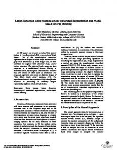
Fig. 1. Pap-smear cell images. (a) Dark blue parts (yellow squares) represent the nucleus. Pale blue parts (green squares) are the cytoplasms. Magenta parts (orange squares) are the background. (b) Touching cells (within the yellow borders). Color ranges from pale to dark blue (within the red border). Nuclei with a non-uniform shape are within the green borders

common method of cervical cancer screening. A pathologist should examine each slide of the Pap smear accurately. The procedure takes away most of the time and energy of pathologists while they review thousands of cells each day. One of the main steps to help the pathologist is to develop an automatic system that can segment and classify cells of the smear's scene in normal and abnormal groups. Since the cervix is wiped out with a swap, the Pap test is classified as an invasive method. It is used only for screening purposes and not for diagnosis. These cells are examined under a microscope for abnormalities [22]. Trained biologists are required to evaluate these tests. In underdeveloped countries, the death rate due to cervical cancer is significantly higher because of the lack of personnel trained in this field and repeated follow-up tests. As a result, women in developed countries have less than 0.1% chance of developing cervical cancer while their counterparts in underdeveloped countries have a 3-5% chance of developing cervical cancer. Nucleus extraction from the Pap smears is the first step for further detection of abnormalities or pre-cancerous cells. Two classes of regions are considered: nucleus regions and other regions

Computación y Sistemas Vol. 16 No. 2, 2012 pp 133-145 ISSN 1405-5546

that include cytoplasm and background (Figure 1).The overall proportion of the nucleus pixels is approximately between 7% and 10%. Cell nuclei are blue (dark to pale) and cytoplasms are bluegreen (Figure 1a). Red blood corpuscles are colored reddish. The spatial configuration and the color of the cells are extremely variable. Isolated or touching cells as well as clustered or overlapping cells can be found (Figure 1b). The automated segmentation of the cell nucleus in Pap smear images is one of the most interesting fields in cytological image analysis [21]. In the last years, cell nuclei segmentation has been extensively studied by several researchers. In [24], frequency domain features are used to detect abnormal cervical cell images. In [27], statistical geometric features, which are computed from several binary thresholded versions of texture images, are used to classify among normal and abnormal cervical cells. Lezoray and Cardot [17] extract the nucleus of the cervical cells using a combination of a color pixel classification scheme k-means and a Bayesian classification with a color watershed segmentation algorithm. In [2], a segmentation scheme and its performance are evaluated using Pap smear samples in the presence of heavy additive noise.

Combined Hierarchical Watershed Segmentation and SVM Classification…135

Developing automated algorithms for segmenting nuclei continues to pose interesting challenges. Much of the difficulty arises from the inherent color and shape variability. The goal of the present work is to develop automated and computationally efficient algorithms that improve upon previous methods using watershed approach [1]. In this work, we propose a hybrid two-step approach to cell segmentation in Pap smear images. The first phase consists of creating a nested hierarchy of partitions, which produces a hierarchical segmentation that uses the spectral and shape information as well as the class information. After constructing the hierarchy of nested partitions by performing waterfall algorithm [13] on the image, we automatically select the most meaningful hierarchical level by using a segmentation quality criterion. The second phase aims at identifying the nucleus and cytoplasm areas by classifying the segments (regions) resulting from the first phase using multiple spectral and shape features, and further merging the neighboring regions belonging to the same class. The selection of individual regions is obtained using a Support Vector Machine (SVM) classifier, based on spectral and shape features. The remainder of the paper is organized as follows. Section 2.2 describes the segmentation algorithm used to segment the images and produce a hierarchy of nested partitions. Section 2.3 proposes an unsupervised segmentation quality criterion to select a set of hierarchical levels, on which SVM classification is applied in Section 2.4 to classify the segmented region in nucleus/non-nucleus and pruning the segmentation errors by merging the adjacent segmented regions which may have been oversegmented. Section 3 presents and discusses the obtained results. Finally, conclusions are presented in Section 4.

2 Materials and Methods 2.1 Pap Smear Cells Databases In order to test the proposed algorithm, images from two Pap-smear cells databases were used. The first database is the image database used in [17], referred to as Lezoray database. In these

images, cells are colored using the international standard of coloration of Papanicolaou [22], and pixels in the ground truth are divided in two classes: nucleus pixels and other pixels. From this database, we used 20 images that contain approximately 160 nuclei. The second database is the Herlev image database [14]. In these images, cells are also colored using the international standard of coloration of Papanicolaou, and pixels in the ground truth are divided in four classes: nucleus pixels, two kinds of cytoplasm pixels, and the background pixels. In our experiments, we consider only two classes: nucleus pixels and other pixels. The Herlev database contains seven kinds of images as described in Table 1. In our experiment, we used 140 images randomly selected, 20 per type. 2.2 Hierarchy of Partitions The waterfall algorithm [4] is used here for producing a nested hierarchy of partitions, P h  {r1h , r2h ,., rmhh }; h  1, n , which preserves the inclusion relationship that each atom of the set

P h  P h1 , implying

P h is a disjoint union of h1

atoms from the set P . For successively creating hierarchical partitions, the waterfall algorithm removes from the current partition (hierarchical level) all the boundaries completely surrounded by higher boundaries. The starting partition is obtained using watershed transform [25], being a morphological segmentation applied on the gradient magnitude of an image in order to guide the watershed lines to follow the crest lines and the real boundaries of the regions. In our implementation, we use the DiZenzo gradient [11], which calculates the maximum rate of change in one pixel based on partial derivatives in RGB color space. For producing the nested hierarchy, in this work, we use the approach proposed in [13], where the saliency measure, E (r  ri  j | ri , rj ) , of a boundary between two neighboring segments ri and rj (being the cost of merging the regions

ri and rj ), is based on a collection of energy

Computación y Sistemas Vol. 16 No.2, 2012 pp 133-145 ISSN 1405-5546

136 Mykel Orozco-Monteagudo, Cosmin Mihai, Hichem Sahli, and Alberto Taboada-Crispi Table 1. Herlev database. Classes 1-3 (242 cells) are normal cells and 4-7 (675 cells) are abnormal ones Class

Category

Cell Type

Count

1 2

Normal

Superficial squamous epithelial

74

Normal

Intermediate squamous epithelial

70

3

Normal

Columnar epithelial

98

4

Abnormal

Mild squamous non-keratinizing dysplasia

182

5

Abnormal

Moderate squamous non-keratinizing dysplasia

146

6

Abnormal

Severe squamous non-keratinizing dysplasia

197

7

Abnormal

Squamous cell carcinoma in situ intermediate

150

Total

functions used to characterize the desired singlesegment properties and the pair-wise segment properties [13].

1 Ehom (r )

1 | Econv (r ) |

E (r  ri  rj ∣ ri , rj )  E (r )  E (ri , rj ) The single segment properties Eq. (1),

E (r ) 

917

· Evarc (r )· c

sign( Econv ( r ))

·1 | Ecomp (r ) |

(2) sign( Ecomp ( r ))

(1)

E (r ) ,

includes segment homogeneity ( Ehom ) , segment convexity ( Econv ) , segment compactness ( Ecomp ) , and color variances ( Evar ) within the segment. c

Taking into account the type of images we are dealing with, in this work we propose the following merging criterion:

E (r  ri  rj ∣ ri , rj ) 

 (ci  c j | ri , rj )· E (r )  E (ri , rj ) 

(3)

Table 2. Region-Based Features Feature Type Morphometrics (69)

Description Generals (9): Major Axis Length, Minor Axis Length, Equivalent Diameter, Orientation, Area, Perimeter, Eccentricity, Convex Area, Solidity. Zernike moments (49): Z i , j ,

i, j  1..12 , i  j

even.

Skeleton features (4): skeleton length, skeleton length-convex hull area ratio, skeleton lengthregion area ratio, and skeleton branch length-skeleton length ratio. Convex hull features (3): eccentricity, shape factor, and fraction of overlap of the convex hull. Textural-based (19)

Grey Level Co-occurrence Matrix based feature or Haralick features (13).

Edge-based (5)

Edge fraction of above-threshold pixels along the edge, measure of edge gradient intensity homogeneity, two measures of edge direction homogeneity, measure of edge direction difference.

Color-based (27)

Nine statistical measures (mean, 0.1-trimmean, max, min, median, standard deviation, interquartile range, skewness, and kurtosis) in the three channels of the RGB color space.

Gabor features (6):

G f , , frequency f {0.06,0.12,0.24} and angle  {0,  / 2}

Computación y Sistemas Vol. 16 No. 2, 2012 pp 133-145 ISSN 1405-5546

Combined Hierarchical Watershed Segmentation and SVM Classification…137

where  (ci  c j | ri , rj ) is a factor favoring the merging of regions with similar classes [19]; E (r ) is the merged region property as defined in [13], it depends on homogeneity, color variance, convexity, and compactness; E (ri , rj ) , the pairwise region property, is defined as:

 b  E (ri , rj )   log   Pri( k ) ·Pr(j k )   k 1 

from [19], the parameter  (ci  c j | ri , rj ) , representing the potential of having neighboring regions with similar class membership, is here defined as follows: (5)

where

ci , c j   1  nucleus, 2  no-nucleus ,

are the classes of ri and r j , respectively, and

p(ci  c j | f (ri ), f (rj )) is the probability that ri and r j belong to the same class, given the feature vectors f (ri ) and f (rj ) . In this work, this probability is estimated using Support Vector Machine (SVM) [10] classification trained using as feature vector f (r ) , the mean of the L, a, and b channels of the regions in the Lab color space. Unfortunately, we cannot directly use the output of the SVM as a probability measure. The output h(f (r )) of the SVM is a distance measure between a test pattern and the separating hyper plane defined by the support vectors. There is no clear relationship with the posterior class probability p(class   | f (r )) that the pattern belongs to the class  . Platt [23] proposed an estimate for this probability by fitting the SVM output h(f (r )) with a sigmoid function:

f (r )

p(ci  c j | f (ri ), f (rj ))  p1 p2  (1  p1 )(1  p2 )

Different

1 1  p(ci  c j | f (ri ), f (rj ))

1 1  exp( A  h(f (r ))  B)

(6)

The parameters A and B are found using maximum likelihood estimation from a training set. Finally, the probability in Eq. (5) is estimated as follows:

(4)

being the Bhattacharyya merging criterion proposed in [7], with the number of bins used b=32.

 (ci  c j | ri , rj ) 

p(class  k | f (r )) 

p1  p(ci  1 | f (ri )) p2  p(c j  1 | f (rj )) are estimated

with

(7)

and using

Eq. (6). The parameters of the SVM classifier have been selected as follows. A linear kernel SVM and Gaussian kernel SVMs (with different values for  ) were trained using a 10-fold crossvalidation. A grid search method was used to select the best parameters of the SVM. The penalty parameter of the error C was tested in C  {2i : i  1..14, } , as well as the parameter of the Gaussian kernel  in

  {2i : i  3..4} . The best performance was obtained for C = 1024 and Gaussian kernel SVM with   0.5 . 2.3 Segmentation Level Selection In order to judge the quality of the image segmentation, three unsupervised criteria were tested: color homogeneity (CH) [12], the method of Borsotti (BOR) [6], and the method of Rosenberger (ROS) [26]. CH combines a region homogeneity measure with an inter-region contrast measure: mh

CH(P ) 

 C (r j 1

h

j 1

) / (mh  1) (8)

mh

 H (r

h j

h j

) / (Card( I )  mh )

Computación y Sistemas Vol. 16 No.2, 2012 pp 133-145 ISSN 1405-5546

138 Mykel Orozco-Monteagudo, Cosmin Mihai, Hichem Sahli, and Alberto Taboada-Crispi

where, for an image I,

Card( I )

denotes the area h j

of the full image (number of pixels). H (r ) is the region homogeneity measure (i.e., local color h h error) of the region rj , while C (rj ) is the interregion separability measure (color difference between adjacent regions), it expresses a tradeoff between the border accuracy of a region and the difference between the region and its neighbors. CH h penalizes those regions with a large color error and a low border contrast. If the color error inside the region is low and the adjacent regions are significantly different (high border contrast), its value is high: the higher the value of CH h , the better the segmentation result is. Using this criterion, the selection of the first hierarchy, often being oversegmented, is excluded. The method of Borsotti (BOR) arose as an improvement of the method of Liu and Yang [18] in order to penalize the phenomenon of oversegmentation.

region disparity is computed by the normalized standard deviation of gray levels in each region. The inter-region disparity computes the dissimilarity of the average gray level of two neighbour regions in the segmentation result. mh 4 2 h m  h  ( ri ) 2 255 i 1 ROS(P h )  2 mh  | g I ( ri h )  g I ( rjh ) |  2   mh (mh  1) i , j 1  512  i j  2

1

h

where g I (rj ) is the average of the gray level of

rjh and  2 (rjh ) is the variance of the gray-level h

of rj . Higher values of the Rosenberger criterion mean a good segmentation. Applied

BOR(P h ) 

mh 4

10 ·Card( I )

P · (9)

2    (Card(rkh ))   Ek2      h Card( rkh )   k 1 1  log(Card( rk ))    mh

where Card() is the size (area) or a region rkh or the image I;

 (Card(rkh )) is the number of

regions having the same size (area) as region rkh ; and Ek is the sum of the Euclidean distances between the RGB color vector of the pixels of rk

r

and the color vector attributed to the region k in the segmentation result. Lower values of the Borsotti criterion mean a good segmentation. In order to harmonize with the other criteria, we used the value of 1  BOR(P h ) as a segmentation quality criterion. The method of Rosenberger (ROS) combines intra- and inter-regions disparities. The intra-

Computación y Sistemas Vol. 16 No. 2, 2012 pp 133-145 ISSN 1405-5546

(10)

h

hierarchy of partitions  {r , r ,., r }; h  1..n , the above criteria h 1

on

h 2

the

h mh

produce, in an unsupervised manner, the best segmentation level. However, most of the time the produced partition does not correspond to the best segmentation level according to the biologists’ criteria. Moreover, applying all the criteria together, they do not often agree on the best segmentation. A suitable approach is to prune the segmentation of the selected partition by merging adjacent regions belonging to the same class. Indeed, as depicted in Figure 2, the selected level shows a cell with two regions, after region-based classification and extra merging, the final segmentation/classification result has been refined. 2.4 SVM Region Classification Support vector machines (SVM) have been proven to be powerful and robust tools for tackling classification tasks [10].Mainly, SVM classification requires the following optimization problem

Combined Hierarchical Watershed Segmentation and SVM Classification…139

max  

 N  1   i  ·  i  j yi y j K (xi , x j )  2 1i , j  N  i 1 

(11)

subject to

0  i  C, with i  1..N

(12)

and N

 i 1

i

yi  0

(13)

where N is the number of cases, yi and y j are 1 or -1 if x i and x j belong to one of the two classes

1 or 2 , respectively, K is the kernel,

and C is a non-negative real number. The best selection of the kernel function is yet a challenging problem in the SVM community. In our work, we used a linear kernel, Gaussian kernels, and polynomial kernels [10]. Unlike mostly used SVM pixel-based classification, we propose to apply SVM on region (segment) features. In order to classify the regions obtained from the segmentation process, a wide set of region features were calculated (Table 2). In an attempt to optimize the dimensionality of the feature set, a subset of features was selected from the feature set (Table 2) via stepwise discriminant analysis [15]. This method uses Wilks' λ statistic to iteratively determine which features are best able to separate the classes from one another in the feature space. Since it is not possible to identify a subset of features that are optimal for classification without training and testing classifiers for all combinations of the input features, optimization of Wilks' λ is a good choice. The nine (out of 116) features that were statistically most significant in terms of their ability to separate the two classes identified using this approach are listed in Table 3. This set was used in the classification phase of the work. Let r  p1 , p2 , , pn  be a given region formed by

the

Fig. 2. Merging after classification. (1) Original image. (2) Label image of the result after waterfall merging. (3) Mosaic image of the result after waterfall merging. (4) Classification result. White parts mean nucleus. (5) Neighbours regions that belong to the same class are merged into one. (6) Manually segmented ground truth

set

of

pixels

p

x1 , y1

(r1 , g1 , b1 ),

Table 3. Selected features using stepwise discriminant analysis Feature

Description

F1

Mean of the green channel

F2

0.1-trim mean of the blue channel

F3

Solidity

F4

Maximum value of the red channel

F5

Edge fraction of pixels along the edges

F6

Edge gradient intensity homogeneity

F7

Edge direction difference

F8

Shape factor of the convex hull

F9

Region area

px2 , y2 (r2 , g2 , b2 ),..., pxn , yn (rn , gn , bn ) . The above features are estimated as follows: Mean of the Green Channel

F1 (r ) 

1 n  gi n i 1

(14)

Trimmed mean of the blue channel

F2 (r ) 

1  bi 0.9·n p1 bi  p2

(15)

Computación y Sistemas Vol. 16 No.2, 2012 pp 133-145 ISSN 1405-5546

140 Mykel Orozco-Monteagudo, Cosmin Mihai, Hichem Sahli, and Alberto Taboada-Crispi

where p1  pb.05 and p2  pb.95 are the .05 and .95 percentile of the blue channel, respectively.

Region Area

F9 (r)  n

Solidity or convexity

F3 (r) 

Area((r)) Area(ConvexHull((r)))

where n is the number of pixels in the region. (16)

3 Results and Discussion

Max value of the red channel

F4 (r)  max{ri }

(17)

1i  n

Edge fraction of pixels along the edges

F5 (r) 

|{ pi : pi  Edge}| Area((r))

(18)

Edge gradient intensity homogeneity Each region is convolved separately with the

1 1 1   kernels N  0 0 0  and W = N' to find   1 1 1   the intensity gradients in the two orthogonal directions of N ( GN ) and W ( GW ). The intensity of the gradient at all points in the image was calculated using A( x, y) 

GN2  GW2

, and a

four-bin histogram was calculated for the values in this edge intensity image. The final feature is the fraction of all values that are in the first bin of this histogram. Edge direction difference For the eight-bin histogram used for measuring the edge direction homogeneity [5], the difference between the bins for an angle and for that angle plus  is calculated by summing bins 1-4 and subtracting the sum of bins 5-8. This difference was normalized by the sum of all eight bins. Convex hull shape factor or convex hull compactness

F8 (r ) 

4· ·Area(ConvexHull((r))) Perimeter(ConvexHull((r))) 2

Computación y Sistemas Vol. 16 No. 2, 2012 pp 133-145 ISSN 1405-5546

(20)

(19)

3.1 Selection of the Segmentation Quality Criterion First, we evaluated the output of the three segmentation selection criteria of Section 2.3 for deciding the best one to be used for the type of images we are dealing with. The evaluation of the segmentation results has been made by using the Vinet measure proposed in [9]. Vinet is a supervised measure widely used to quantify the distance between two segmentations A and B, with m and n regions, respectively, of an image with N pixels. First, a label superposition table is computed: Tij  ∣ Ai  B j ∣ with 0  i  m and

0  j  n . The maximum of this matrix gives the two most similar regions extracted from A and B, respectively. The similarity criterion is defined by C0  max(Tij ) with 0  i  m and 0  j  n . The research of the second maximum (without taking into account the two last regions) gives the similarity criterion C1 and so on to Ck 1 , where

k  min(m, n).

The dissimilarity measure between the two segmentations A and B is given by

D( A, B)  1 

1 N

k 1

C i 0

i

(21)

When one of the segmentations (B, for example) is a ground truth, then lower values of the Vinet measure mean a good segmentation (close to the reference). Instead of the greedy approach to calculate the values of Ci , i  1..min(n, m) , the Hungarian algorithm [20] can be used. The Hungarian algorithm increases the computational cost but the accuracy of the measure will increase too.

Combined Hierarchical Watershed Segmentation and SVM Classification…141

3.2 Evaluation on the Lezoray Database

Table 4 shows the evaluation results of the segmentation evaluation criteria applied on the images from the Lezoray database. The selected hieratical level, provided by each of the evaluation criterions, has been compared to a manually delineated segmentation using the Vinet measure. From the segmentation point of view, the best results were obtained using the Borsotti criterion.

The proposed approach was applied to the twenty images that contain approximately 160 nuclei. The evaluation of the segmentations was done using a leave-one-out cross-validation approach with the Vinet distance with respect to the manually obtained segmentation. Training of the SVM was done using the SVM-KM toolbox [8]. Figure 3 illustrates the proposed approach in one of the tested images. The first row depicts some hierarchical levels along with their BOR criterion and the number of regions. As it can be noticed, the hierarchical Level 1 is the best according to the BOR criterion. Moreover, the BOR criterion between the first three levels is almost identical. After SVM classification and

Table 4. Results for different level selection criteria Level Selection Criterion

Vinet Measure

Method of Rosenberger

0.0281

Method of Borsotti

0.0223

Color Homogeneity

0.0252

Table 5. Confusion matrices - SVM classification of the regions shown in Figure 3 Level 1 2 3 6

Non-Nucleus Non-Nucleus

Nucleus

290 (100.0 %)

0 (0.00 %)

Nucleus

4 (23.53 %)

13 (76.47 %)

Non-Nucleus

151 (100.0 %)

0 (0.00 %)

Nucleus

1 (9.09 %)

10 (90.91 %)

Non-Nucleus

91 (98.91 %)

1 (1.09 %)

Nucleus

0 (0.00 %)

6 (100.0 %)

Non-Nucleus

29 (96.67 %)

1 (3.33 %)

Nucleus

0 (0.00 %)

1 (100.0 %)

Table 6. Lezoray database - Overall SVM Classifier

Vinet Measure

Accuracy

F-measure

Linear Kernel

0.0223

0.9733

0.9853

Gaussian Kernel σ = 0.5

0.0494

0.9109

0.9587

Gaussian Kernel σ = 1

0.0456

0.9235

0.9644

Gaussian Kernel σ = 2

0.0407

0.9448

0.9704

Gaussian Kernel σ = 4

0.0323

0.9592

0.9781

Gaussian Kernel σ = 8

0.0274

0.9668

0.9821

Linear Kernel d = 2

0.0375

0.9546

0.9750

Linear Kernel d = 3

0.0528

0.9552

0.9758

CCW

0.0455

0.9571

0.6445

GEE

0.0243

0.9784

0.9880

SVMP

0.0356

0.9743

0.8601

Computación y Sistemas Vol. 16 No.2, 2012 pp 133-145 ISSN 1405-5546

142 Mykel Orozco-Monteagudo, Cosmin Mihai, Hichem Sahli, and Alberto Taboada-Crispi

Original Image

Ground Truth (9 nuclei)

Level 1 BOR = 0.99983 307 regions

Level 2 BOR = 0.99973 162 regions

BOR = 0.9905 V = 0.023 9 Nuclei

BOR = 0.9927 V = 0.019 9 Nuclei

Level 3 BOR = 0.99964 98 regions

Level 6 BOR = 0.99953 31 regions

BOR = 0.9870 V = 0.017 9 Nuclei

BOR = 0.9875 V = 0.029 9 Nuclei

Fig. 3. Illustration of the approach. (Upper-Left) Original Image. (Bottom-Left) Ground Truth. (Upper-Right) Four Hierarchical Levels. (Bottom-Right) Results after classification and second merging

merging of the neighboring regions belonging to the same class (the second and third rows of Figure 3), the hierarchical Level 2 gives better segmentation results with respect to the BOR criterion and the Vinet distance, V. Table 5 gives quantitative results of the segmentations of Figure 3 by the confusion matrixes. In Level 1, both nucleus and non-nucleus regions are oversegmented and the classification accuracy is the lowest. On the opposite, Level 6 is undersegmented but the classification accuracy is the best. The best compromise between segmentation and classification results is obtained in Level 3. The averages of the Vinet measure, classification accuracy and F-measure over all the Lezoray images are summarized in Table 6. Following the Vinet measure, the best results were obtained using the SVM classifier with a

Computación y Sistemas Vol. 16 No. 2, 2012 pp 133-145 ISSN 1405-5546

linear kernel. The segmentation and classification accuracy can be considered good due to the intra-expert distance between 0.01 and 0.04 [3]. Small and in-border nuclei are the principal sources of errors. Table 7 shows the confusion matrix for the SVM classification performance using a linear kernel. From the object classification point of view, the obtained specificity (98.49%) greater than the sensibility (90.84%) means that the proposed classifier tends to classify as nonnucleus regions a nucleus regions but not the opposite. Table 7. Lezoray database - Confusion Matrix Non-Nucleus

Nucleus

Non-Nucleus

98.49%

1.51%

Nucleus

9.16%

90.84%

Combined Hierarchical Watershed Segmentation and SVM Classification…143

(a)

(b)

(c)

(d)

Fig. 4. Segmentation and classification results for an image from the Herlev database. (a) Original image. (b) Mosaic image after segmentation. (c) Nucleus region classification. (d) Ground truth

To further assess our results, we give in the last rows of Table 6 the results obtained using three state of art methods, namely, the Cooperative color watershed proposed in [17] (CCW), the Hierarchical Segmentation of [13] (GEE), and a Pixel-based SVM classification (SVMP) [10]. As it can be seen from Table 6, the proposed approach produces good results. 3.3 Evaluation on the Herlev Database The evaluation of the approach using different SVM kernels has been also made on the Herlev database as shown in Table 8. In order to compare with the results reported in [16] (KAL), the Zijdenbos measure [28] was used to evaluate the segmentation quality with respect to the ground truth. The Zijdenbos measure is defined as the ratio of twice the common area between two regions to the sum of the individual areas. When the Zijdenbos measure is greater than 0.7, there is an excellent agreement between Table 8. Herlev database - Overall evaluation SVM Classifier

Zijdenbos Measure

Accuracy

Fmeasure

Linear Kernel

0.7152

0.9385

0.9663

Gaussian Kernel σ=1

0.9325

0.9978

0.9988

Gaussian Kernel σ = 10

0.8046

KAL

0.9232

both segmentations. As it can be seen, we obtain comparable results to the ones applied to the Lezoray database. Good results were obtained in all the approaches but very good results were achieved by using a Gaussian kernel with unitary variance.

4 Conclusions In this work, we tested a hybrid segmentationclassification approach to automatically select and improve the segmentation of nucleus of cells in images of the Papanicolaou test using nested hierarchical portioning, segmentation level selection, and an SVM classifier for the final merging to avoid over-segmentation. The segmentation was done by a morphological algorithm (watershed) and a hierarchical merging algorithm (waterfall) based on spectral information and shape information, as well as the class information. A SVM classifier was used to separate two classes of regions, nucleus and not nucleus regions (cytoplasm and background) using appropriate set of features (morphometric, edge-based, and convex hull-based). The proposed approach allows pruning most of the wrongly segmented cells avoiding over/under segmentation and produces segmentation closer to what is expected by expert pathologists.

References 0.9655

0.9812

1.

Angulo, J. & Serra, J. (2005). Segmentación de imágenes en color utilizando histogramas bivariables en espacios color polares

Computación y Sistemas Vol. 16 No.2, 2012 pp 133-145 ISSN 1405-5546

144 Mykel Orozco-Monteagudo, Cosmin Mihai, Hichem Sahli, and Alberto Taboada-Crispi luminancia/saturación/matiz. Computación y Sistemas, 8(4), 303–316. 2. Bak, E., Najarian, K., & Brockway, J.P. (2004). Efficient segmentation framework of cell images in th noise environments. 26 Annual International Conference of the IEEE Engineering in Medicine and Biology Society (IEMBS '04), San Francisco, California, USA, 1802–1805. 3. Bergen, T., Steckhan, D., Wittenberg, T., & Zerfass, T. (2008). Segmentation of leukocytes th and erythrocytes in blood smear images. 30 Annual International Conference of the IEEE Engineering in Medicine and Biology Society (EMBS 2008), Vancouver, Canada, 3075–3078. 4. Beucher, S. & Meyer, F. (1993). The morphological approach to segmentation: the watershed transformation. Mathematical Morphology in Image Processing (433–482). New York: M. Dekker. 5. Boland, M.V. & Murphy, R.F. (2001). A neural network classifier capable of recognizing the patterns of all major subcellular structures in fluorescence microscope images of HeLa cells. Bioinformatics, 17(12), 1213–1223. 6. Borsotti, M., Campadelli, P., & Schettini, R. (1998). Quantitative evaluation of color image segmentation results. Pattern Recognition Letters, 19(8), 741–747. 7. Calderero, F. & Marques, F. (2008). General region merging approaches based on information th theory statistical measures. 15 IEEE International Conference on Image Processing (ICIP 2008), San Diego, CA, USA, 3016–3019. 8. Canu, S., Grandvalet, Y., & Rakotomamonjy, A. (2003). SVM and Kernel Methods MATLAB Toolbox. Perception de Systemes et Information, INSA de Rouen, France. 9. Cohen, L., Vinet, L., Sander, P.T., & Gagalowicz, A. (1989). Hierarchical regional based stereo matching. IEEE Computer Society Conference on Computer Vision and Pattern Recognition (CVPR’89), San Diego, CA, USA, 416–421. 10. Cristianini, N. & Shawe-Taylor, J. (2000). An Introduction to Support Vector Machines and other kernel-based learning methods. Cambridge; New York: Cambridge University Press. 11. Geerinck, T., Mihai, C., Jabloun, M., Vanhamel, I., & Sahli, H. (2009). Multi-scale image analysis of

Computación y Sistemas Vol. 16 No. 2, 2012 pp 133-145 ISSN 1405-5546

12.

13.

14.

15.

16.

17.

18.

19.

20.

21.

22.

satellite data using perceptual grouping. IEEE International Geoscience and Remote Sensing Symposium. Geerinck, T., Sahli, H., Henderickx, D., Vanhamel, I., & Enescu, V. (2009). Modeling Attention and Perceptual Grouping to Salient Objects. Attention in Cognitive. Lecture Notes in Computer Science, 5395, 166–182. Jantzen, J., Norup, J., Dounias, G., & Bjerregaard, B. (2005). Pap-smear Benchmark Data for Pattern Classification. Nature inspired Smart Information Systems (NiSIS 2005), Albufeira, Portugal, 1–9. Jennrich, R.I. & Sampson, P. (1960). Stepwise discriminant analysis. Mathematical methods for digital computers, 339-358. Kale, A. & Aksoy, S. (2010). Segmentation of th Cervical Cell Images. 20 International Conference on Pattern Recognition (ICPR). Istanbul, Turkey, 2399–2402. Lezoray, O. & Cardot, H. (2002). Cooperation of color pixel classification schemes and color watershed: a study for microscopic images. IEEE Transactions on Image Processing, 11(7), 783– 789. Liu, J. & Yang, Y.H. (1994). Multiresolution color image segmentation. IEEE Transactions on Pattern Analysis and Machine Intelligence, 16(7), 689–700. Lucchi, A., Smith, K., Achanta, R., Lepetit, V., & Fua, P. (2010). A Fully Automated Approach to Segmentation of Irregularly Shaped Cellular th Structures in EM Images. 13 International Conference on Medical Image Computing and Computer-Assisted Intervention, Part II (MICCAI’10), Beijing, China, 463–471. Munkres, J. (1957). Algorithms for the assignment and transportation problems. Journal of the Society for Industrial and Applied Mathematics, 5(1), 32– 38. Pantanowitz, L., Hornish, M., & Goulart, R.A. (2010). The impact of digital imaging in the field of cytopathology. Cytojournal, 6(6). Papanicolaou, G.N. & Traut, H.F. (1943). Diagnosis of uterine cancer by the vaginal smear. Yale Journal of Biology and medicine, 15(6), 924. Platt, J.C. (2000). Probabilities for SV Machines. Advances in large margin classifiers (61–74), Cambridge, Mass.: MIT Press.

Combined Hierarchical Watershed Segmentation and SVM Classification…145 23. Ricketts, I.W., Banda-Gamboa, H., Cairns, A.Y., & Hussein, K. (1992). Automatic classification of cervical cells-using the frequency domain. IEE Colloquium on Applications of Image Processing in Mass Health Screening, London, UK, 9/1–9/4. 24. Roerdink, J.B.T.M. & Meijster, A. (2000). The watershed transform: Definitions, algorithms and parallelization strategies. Fundamenta Informaticae- Special issue on Mathematical morphology, 41(1-2), 187–228. 25. Rosenberger, C. (1999). Mise en oeuvre d'un systeme adaptatif de segmentation d'images. Thèse de doctorat, Universite de Rennes 1, Rennes, Francia. 26. Walker, R.F. & Jackway, P.T. (1996). Statistical geometric features-extensions for cytological th texture analysis. 13 International Conference on Pattern Recognition, Vienna, Austria, 2, 790–794. 27. Zenzo, S.D. (1986). A note on the gradient of a multi-image. Computer Vision, Graphics, Image Processing, 33(1), 116–125. 28. Zijdenbos, A.P., Dawant, B.M., Margolin, R.A., & Palmer, A.C. (1994). Morphometric analysis of white matter lesions in MR images: method and validation. IEEE Transactions on Medical Imaging, 13(4), 716–724.

Mykel Orozco Monteagudo received his B.S. and M. Sc. degrees in Computer Sciences from Universidad Central de Las Villas (UCLV), Cuba, in 2002 and 2006, respectively. Since 2005, he has been in the Center of Studies on Electronic and Information Technologies (CEETI) as an Auxiliary Professor. His research interests are image processing and pattern recognition for biomedical applications. Cosmin Mihai received his Software Engineering degree from Universitatea Politehnica din București in 2003. At present, he works as a Software Design Engineer at Honeywell Aerospace, Brno, Czech Republic. His main research interests include computational vision,

image and motion segmentation, and machine learning.

Hichem Sahli received his Ph.D. degree in Computer Sciences from the Ecole Nationale Supérieure de Physique Strasbourg, Strasbourg, France, in 1991. He joined the Department of CAD and Robotics of the Ecole des Mines de Paris in 1992. In 1999, he moved to the Vrije Universiteit Brussel, Brussels, Belgium, where currently he is a Professor at the Department of Electronics and Informatics. He coordinates the research team in Computer Vision and Audio Visual Signal Processing. His main research interests include computational vision, image and motion segmentation, machine learning, visual reconstruction, and optimization. Dr. Sahli is a member of IEEE and ACM.

Alberto Taboada-Crispi is a graduate of Electronic Engineering (Universidad Central de Las Villas, UCLV, 1985), Master in Electronics (UCLV, 1997), and Ph.D. (University of New Brunswick, Canada, 2002). He worked as a Specialist for Medical and Laboratory Equipment in the Villa Clara Provincial Hospital from 1985 to 1988. Since then, he has been with the Faculty of Electrical Engineering (FIE) of the UCLV. Currently, he is a Professor and Researcher, and the Director of the Center for Studies on Electronics and Information Technologies (CEETI), FIE, UCLV. His topics of interest include instrumentation, analog and digital processing of signals and images, and biomedical applications. Article received on 30/04/2011; accepted on 29/02/2012.

Computación y Sistemas Vol. 16 No.2, 2012 pp 133-145 ISSN 1405-5546