stances during the feature pruning. While standard selection algorithms often optimize the accuracy to discriminate the set of solu tions, we use in this paper a ...
UNCERTAINTY IN ARTIFICIAL INTELLIGENCE PROCEEDINGS 2000
533
Combining Feature and Example Pruning by Uncertainty Minimization
Marc Sebban
Richard Nock
Dpt of SJE
Dept of Mathematics and CS
French West Indies and Guiana University
French West Indies and Guiana University
97159
Pointe-a-Pitre Cedex
Abstract
97159
Pointe-a-Pitre Cedex
ber of instances
( John, 1995)
& Shavlik,
used during induction.
1996)
or features
( Cherkauer ( IBL ) ,
We focus in this paper on dataset reduction
For Instance-Based Learning algorithms
techniques for use in k-nearest neighbor clas
reduction techniques are also crucial even if they do
sification. In such a context,
not pursue the same aim.
feature and pro
data
While Nearest-Neighbor
selections have always been indepen
( NN) algorithms are known to be very efficient for solv
dently treated by the standard storage reduc
ing classification tasks, this effectiveness is counter
totype
tion algorithms. While this certifying is the
balanced by large computational and storage require
oretically justified by the fact that each sub
ments. The goal of reduction procedures consists then
problem is NP-hard, we assume in this paper
in reducing these computational and storage costs. In
that a joint storage reduction is in fact more
this paper, we only focus on these storage reduction
intuitive and can in practice provide bet
algorithms for use in a NN classification system.
ter results than two independent processes. Moreover, it avoids a lot of distance calcu lations by progressively removing useless in stances during the feature pruning.
While
standard selection algorithms often optimize the accuracy to discriminate the set of solu tions, we use in this paper a criterion based on an uncertainty measure within a nearest neighbor graph. This choice comes from re cent results that have proven that accuracy is
The selection problem has been treated during last decades according to two different ways to proceed:
(i)
the reduction algorithm is employed to reduce the size n
of the learning sample, called Prototype Selection
( PS ) ( Aha, Kibler & Albert, 1991; Brodley & Friedl, 1996; Gates, 1972; Hart, 1968; Wilson & Martinez, 1997; Sebban & Nock, 2000), ( ii) the algorithm tries to reduce the dimension p of the representation space in which the
n
instances are inserted, called Feature
Selection
( FS) ( John, Kohavi & Pfleger, 1994; & Sahami, 1996; Skalak, 1994; Sebban, 1999).
Koller
removed if its deletion improves information
Surprisingly, as far as we know, except Skalak
(1994)
of the graph. Numerous experiments are pre
who independently presents FS and PS algorithms in
not always the suitable criterion to optimize. In our approach, a feature or an instance is
sented in this paper and a statistical analysis
a same paper, and Blum and Langley
shows the relevance of our approach, and its
pose independent surveys of standard methods, no ap
tolerance in the presence of noise.
(1997)
who pro
proach has attempted to globally treat the reduction problem, and to control these two degrees of freedom in the same time. Yet, Blum and Langley
1
INTRODUCTION
(1997)
un
derline the necessity to further theoretically analyze the ways in which instance selection can aid the fea
With the development of modern databases, data re
ture selection process.
duction techniques are commonly used for solving ma
for studies designed to help understand and quantify
chine learning problems. In the Knowledge Discovery
Authors emphasize the need
the relationship that relates FS and PS. In this paper,
in Databases field ( KDD) , the human comprehensibil
we attempt to deal with the storage reduction taken
ity of the model is as important as the predictive ac
as a whole. Conceptually, the task is not so difficult,
curacy of decision trees. To address the issue of human
because PS and FS algorithms share the same aim
comprehensibility and build smaller trees, data reduc
and often optimize the same criterion. Theoretically
tion techniques has been proposed to reduce the num-
speaking, the problem is in fact much more difficult: it
UNCERTAINTY IN ARTIFICIAL INTELLIGENCE PROCEEDINGS 2000
534
can be actually proven that FS and PS are both NP hard problems
(reductions
0 I
from the Set Cover prob
lem ) . To cope with this difficulty, PS or FS algorithms propose heuristics to limit the search through the so
lution space, optimizing an adapted criterion. In this paper, we propose to extend this strategy to a joint reduction algorithm because it is still NP-hard. The majority of reduction methods maximize the accuracy on the learning sample. While the accuracy optimiza tion is certainly a way to limit further processing's er rors on testing, recent works have proven that it is not always the suitable criterion to optimize. In Kearns and Mansour
(1996),
a formal proof is given that ex
plains why Gini criterion and the entropy should be
F igure
1:
Four categories of irrelevant instances re
moved by a prototype selection algorithm
optimized instead of the accuracy when a top-down induction algorithm is used to grow a decision tree. In this paper, we propose to extend this principle to a
information. The
joint data reduction. Our approach minimizes a global
concentrated areas between the border and the cen
third
instances belong to the most
uncertainty (based on an entropy ) within a kNN graph
ter of each class. They are not irrelevant by the risk
In such a graph, a given w instance is not only con
second.
nected to its kNN, but also to instances that have w
sense that removing such examples would not lead to
built on the learning set (see section
in their neighborhood Martinez
(1997)).
2 for definitions) .
(called associates
in Wilson &
The interest of this procedure con
they bring during the generalization, such as for the They constitute irrelevant instances in the
a misclassification of an unseen instance. The last
egory
concerns mislabeled instances (instance
4
cat
on the
sists in better assessing the field of action of each in
figure ) . Labeling error can come from variable mea
stance
surement techniques, typing errors, etc. In statistics,
w
and then minimizing the risk of a wrongly
elimination.
We have already independently tested
our uncertainty criterion in the PS
2000) and in section
FS
3
(Sebban, 1999)
(Sebban
& Nock,
fields. We briefly recall
the main results obtained with these two
approaches.
Afterwards, we propose in section
4
to
mislabeled instances belong to a larger class called out
liers, i.e.
they do not follow the same model of the
rest of the data. It includes not only erroneous data but also "surprising" data
(John, 1995).
A data re
duction technique is called robust if it can withstand
combine and extend their principles in one and a same
outliers in data. In such a context, we think that mis
mixed reduction algorithm. We give some arguments
labeled instances must be eliminated prior to applying
that justify the use of this joint procedure rather than
a given learning algorithm, even if a separate analysis
two independent processes. Our mixed backward algo
could reveal information about special cases in which
rithm, called
(FS
+
PS)RCG,
alternates the deletion
of an irrelevant feature, and the removal of irrelevant
the model does not work.
The third category must
also be removed because it brings no relevant infor
instances. A survey of feature relevance definitions is
mation.
proposed in
With regard
progressive elimination of these instances during our
to prototypes, we cluster in this paper irrelevant in
mixed procedure. The remaining irrelevant instances
(Blum
and Langley,
1997).
stances in four main categories. We detail them
(see
We are then essentially concerned with the
will be removed later
( when
the representation space
figure 1) because the nature of each irrelevant instance
will be stabilized) , because their status could evolve
will determine the stage of its deletion in our algo
during the reduction of the representation space.
rithm. The
first
belong to regions in the feature space with
very few elements
(see
instance
1
on figure
1).
Even
2
THEORETICAL FRAMEWORK
if most of these few points belong to the same class, their vote is statistically a poor estimator, and a little noise might affect dramatically their contribution. It is also common in statistical analyses to search and remove such points, in regression, parametric estima tions, etc. The
second
belong to regions where votes
can be assimilated as being randomized. Local densi ties are evenly distributed with respect to the overall class distributions, which makes such regions with no
In this paper, we do not use the accuracy as criterion. Our performance measure is based on a quadratic en tropy. The strategy consists in measuring information around each instance, and deducing a global uncer tainty within the learning sample. The information is represented by the edges linked to each instance in the kNN unoriented graph.
This way to proceed brings
several advantages in comparison with the accuracy:
535
UNCERTAINTY IN ARTIFICIAL INTELLIGENCE PROCEEDINGS 2000
•
contrary to the accuracy, our criterion does not depend on a
•
ad hoc
learning algorithm,
Table
1:
20
Average accuracy on
databases; p is the
average size of the original sets, and p
with the accuracy, an instance is correctly classi
the reduced space by
*
is the size of
FSRCG
fied or misclassified. The use of our criterion al lows us to have a continuous certainty measure, •
we show below that our criterion has statistical properties which establish a theoretical frame work for halting search,
•
around a given instance w, we take into account
Uo is the uncertainty a priori distribution.
not only the neighbors of w but also instances
where
which have w in their neighborhood. Therefore, it
the
allows to better assess the field of action of each
c Uo =E �(1- �) j=l
instance.
Definition 1 The Quadratic Entropy is a function QE from [0, W in [0, 1], QE : S c
__.
[0, 1]
c (1'1, .. ,"fc)--> QE(("fl, .. ,')'c))= L ')'j(l- 'Yj) j=l
= {wj
ES
I w; is linked by an edge to the kNN graph}
Wj
3
Light and Margolin
(1971)
Y (w1 )
!!i.i.. (1- !!i.i.. ) n ·. n· '·
=
show that the distribution
degrees of freedom. Rather than
INDEPENDENT FEATURE AND PROTOTYPE SELECTIONS
3.1
FSRCG
In this feature selection algorithm, proposed in Seb
(1999),
we start without attribute
(forward
algo
(ntaking Ut ot
as criterion, we define the following criterion:
Definiti on 5 The Relative Certainty Gain in a k NN graph is defined as being:
(1994),
Utot·
According to John,
this approach is a filter
model, because it filters out irrelevant attributes be
fore the induction process occurs (see also the following filter models: Koller & Sahami,
1996;
Sebban,
1999).
A filter method contrasts with wrapper models which use an induction algorithm
(and
then its accuracy )
(John, Ko 1994). The pseudocode of FSRCG is presented in figure 2, where>> means "statistically higher". Table 1 recalls a comparison be tween FSRCG in a 1NN graph, a standard wrapper model optimizing the accuracy (Ace. in the table ) , and a model using all the attributes ( All) (for details on experiments, see Sebban (1999)). The comparison on 20 benchmarks coming for the majority from the UCI to assess the relevance of feature subsets havi and Pfleger,
of the relative quadratic entropy gain is a x2 with
1)(c- 1)
where the
is able to assess the effect of an instance
duce the global uncertainty
n
..
RCG
Kohavi and Pfleger
n =L n;. 2card {E} i=l where E is the set of all the edges in the kNN graph, and n the number of instances. where
Y j} , i.e. Yi
=
rithm ) and select the best feature that allows to re
Definition 4 the total uncertainty U tot in the learn ing sample is defined as being:
'
Y (w; )
and will provide an efficient criterion for halting search
ban
and n;j = card{w1 E N (w; ) I Y (wl ) = Yi} where describes the class of w1 among c classes.
i=l .. j=l
card{w; I
through the solution space.
in
where n;. = card{N(w;)}
'""" ... L... utot ='""" L... !!:..i. n
=
statistical properties constitute a rigorous framework
c Uloc (w·' ) ='""" (1- !!i.i.. ) L... !!i.i.. n· n·.. j=l ,.
c
nj
label of w; is the class Thus,
Definition 3 the local uncertainty Uloc(w;) for a given w; instance belonging to S is defined as being:
n
where
or a feature deletion on the global uncertainty. These
Definiti on 2 The neighborhood N (w; ) in a k NN graph of a given w; instance belonging to a sample S is: N ( w; )
computed directly from
1994;
Skalak,
repository was done using a 5-folds Cross-Validation procedure and applying a
1NN
classifier.
A statistical analysis allows us to make the following remarks:
1.
On average,
FSRCG
presents better results than
UNCERTAINTY IN ARTIFICIAL INTELLIGENCE PROCEEDINGS 2000
536
FSRCG ALGORITHM RCG = 0 E = 0; X={X�, X2, ..., Xp}
Stop=false
Repeat
X; E X do Compute RCG; in EUX; X min with RCG min= Max{RCGj} RCGmin>> RCG then X=X -{Xmin} E=E U {Xmin} RCG�RCGmin
For each Select If
else Stop:=true Until Stop=true Return the feature subset
E
Figure 2: Pseudocode of F S RCG a standard feature selection algorithm optimizing the accuracy. The mean gain of FSRCG is about +1.6 (76.69 vs 75.05). Using a Student paired t test, we find that FSRCG is statistically higher than Ace. with a critical risk near 5%, that is highly significant.
2. The advantage of FSRCG is confirmed by analyz ing the results of All Attributes (All}. FSRCG allows a better accuracy, on average +3.0, that is also highly significant. Using a Student paired t test, we find actually a critical risk near 0.6%, while the standard wrapper is better with a risk about 17%, that is less significant. 3. Globally, FSRCG reduces the number of features (8.4 vs 15.7 on average) and then the storage re quirements for a kNN classifier. 3.2
PSRCG
The high majority of PS algorithms uses the accuracy to assess the effect of an instance deletion ( see Hart, 1968; Gates, 1972; Aha, Kibler & Albert, 1991; Skalak, 1994; Wilson & Martinez 1997). In Hart (1968), the author proposes a Condensed NN Rule ( CNN) to find a Consistent Subset, CS, which correctly classifies all oft'-� remaining points in the sample set. The Reduced NN Rule (RNN) proposed by Gates (1972) searches in Hart's CS for the minimal subset which correctly clas sifies all the learning instances. In Aha, Kibler and Albert (1991), the IB2 algorithm is quite similar to Hart's CNN rule, except it does not repeat the process after the first pass. Skalak (1994) proposes two algo rithms to find sets of prototypes for NN classification. The first one is a Monte Carlo sampling algorithm, and the second applies random mutation hill climbing. Fi nally, in the algorithm RT3 of Wilson and Martinez (1997) (called DROP 3 in Wilson and Martinez (1998) and its extensions DROP4 and DROP S), an instance w; is removed if its removal does not hurt the classi-
Figure 3: The deletion of an instance results in some local modifications of the neighborhood. Only instances (1,2,3 and 4) concerned by the deleted point (the black ball) are affected by these modifications. fication of the instances remaining in the sample set, notably instances that have w; in their neighborhood ( called associates). In our prototype selection algorithm, proposed in Seb ban & Nock (2000), we insert our information crite rion in a PS procedure. At each deletion, we have to compute again some local uncertainties, and analyze the effect of the removal on the remaining informa tion ( see figure 3). This update is relatively computa tionally unexpensive for the reason that only points in the neighborhood of the removed instance will be con cerned by a modification. Updating a given Utoc(Wj) after removing w; does not cost more than O (n;.), a complexity which can be further decreased by the use of sophisticated data structures such as k-d trees ( Sproull, 1991). Our strategy consists in starting from the whole set of instances and searching for the worst instance which allows, once deleted, to improve the in formation. An instance is eliminated at the step t if and only if two conditions are filled: (1) the Relative Certainty Gain after the deletion is better than before, i.e. RCGt>> RCGt-1 and (2) RCGt>> 0. Once this first procedure is finished ( consisting in a way in deleting border instances) , our algorithm exe cutes a post-process consisting in removing the center of the remaining clusters and mislabeled instances. To do that, we increase the geometrical constraint by ris ing the neighborhood size (k+1), and remove instances that still have a local uncertainty Utoc(w;)= 0. The pseudocode of P SRCG is presented in figure 4. From table 2 which presents the summary of a wide com parison study ( with k= 5) between the previous cited standard PS algorithms ( see in Sebban and Nock, 2000 for more details) , we can make the following remarks:
1. C NN and RNN, which are known to be sensi tive to noise fall much in accuracy after the in-
UNCERTAINTY IN ARTIFICIAL INTELLIGENCE PROCEEDINGS 2000
537
Table 2: Comparison between PSRCG and existing PS algorithms on 20 datasets; 5NN is inserted for comparison
5NN
CNN size(%) l AcccNN 44 I 72.4
Ace
75.7
RNN size(%) I AccRNN 41 I 71.9
PSRCG ALGORITHM t f- 0; Np l S I Build the kNN graph on the learning set RCGl = Uo-Ut9t
w
with the
If 2 instances
75.9
74.6
Algorithm kNN
t+-t + 1 Select
Carlo
n8=100
PS
Uo
Repeat
M.
AccpsRCG
RT3
size(%) I 12.6 I
AccRT3 73.7
Table 3: Average accuracy and storage requirements when noise is inserted
=
Compute RCG1
PSRCG
size(%) I 44.9 I
ma.x(Uloc(wj)) have the same Uloc
Noise-Free
Size% Noisy
Size%
74.4
100.0
69.0
PSRCG
74.7
44.5
73.4
47.8
RT3
72.5
11.0
69.7
10.5
100.0
select the example having the smallest number of neighbors Local modifications of the kNN graph Compute RCGt+1 after removing
Np
w
NP -1
+-
Until CRCGt+l < RCGt) or not(RCGt+l>>
0)
Remove instances having a null uncertainty with their
(k + 1)-NN
Return the prototype set with
Figure 4: Pseudocode of
NP
instances
PSRCG
stance reduction (the difference is statistically sig nificant). 2. The Monte Carlo method (Skalak) presents inter esting results despite the constraint to provide in advance the number of samples and the number of prototypes (here Np)· is suited to dramatically decrease the size of the learning set (12 .6 % on average). In compen sation, the accuracy in generalization is a little reduced (about -2.0).
3. RT3
4.
PSRCG requires a higher storage (44.9% on aver age), but interestingly, it allows here to slightly improve the accuracy (75.9% vs 75.7%) of the standard kNN classifier, even if a Student paired t test shows that the two methods are statisti cally indistinguishable. Nevertheless, it confirms that PSRCG seems to be a good solution to select relevant prototypes and then reduce the memory requirements, while not compromising the gener alization accuracy.
We have also tested the sensitivity of our algorithm to noise. A classical approach to deal with this problem consists in adding artificially some noise in the data
set. This was done here by randomly changing the out put class of 10% of the learning instances. We did not test the CN N and RN N algorithms on noisy samples, because they are known to be very sensitive to noise (W ilson & Martinez, 1998). Table 3 shows the average accuracy and storage requirements for PSRCG, RT3, and the basic kNN over the datasets already tested. has the highest accuracy (73.4%) of the three algorithms, while storage requirements are relatively controlled. It presents a good noise tolerance because it does not fall much in accuracy (-1.3 for 10% of noise), versus -2.8 for RT3 and -5.4 for the basic kNN. PSRCG
COMBINING FEATURE A ND
4
PROTOTYPE SELECTION
4.1
PRESENTATION
The previous section has recalled that our information criterion seems to be efficient in a storage (feature or prototype) reduction algorithm. Since we optimize in both algorithms the same criterion, it is in the nature of things to combine the two approaches in one and the same selection algorithm. Nevertheless, this iso lated argument is not very convincing and does not give information about the way to proceed. The fol lowing arguments will certainly bring a higher signifi cance in favor of a combined selection, rather than two independent procedures. •
By alternatively reducing the number of features and instances, we reduce the algorithm com plexity. The computation of a local uncertainty Uloc(w) (useful for PS) is actually not very costly because it is done during the RCG evaluation. Then, this additional PS treatment is not compu tationally expensive. On the other hand, this pro-
UNCERTAINTY IN ARTIFICIAL INTELLIGENCE PROCEEDINGS 2000
538
gressive instance reduction will decrease a lot the future computations in the smaller representation space, avoiding numerous distance calculations on the removal examples. In total, a combined selec tion will be certainly less expensive than a feature selection followed by a only one global prototype selection. •
•
A progressive instance reduction during the fea ture pruning can also avoid to reach a local opti mum during feature pruning. The interest of our algorithm is that it takes into account two crite ria, one local (Uloc(w)), the other global (RCG). It consists in improving local information, with out damaging the global uncertainty. The exper iments will confirm this remark. Mixed approach attempts has been rare in this field, despite a common goal in PS and FS, (i.e. reducing the storage requirement) and obvious in teractions (Blum and Langley, 1997).
Rather than roughly deleting a lot of instances after each stage of the feature reduction, we prefer to apply a moderate procedure which consists in sequentially re moving only mislabeleil instances and center examples during the mixed procedure. Actually, the status of these points will probably not evolve during the stor age reduction. In our approach, we define a mislabeled instance as a w example having in its N(w) (including its associates) only points belonging to a different class of w, i.e. w is mislabeled if and only if Y(w) f Y(wj) , Vwi E N(w) We can believe that few mislabeled instances in a dimension could become informative in a (p 1) dimensional space.
p
-
Concerning instances that belong to the center of classes, their usefulness is not very important, and moreover they probably will not be disturbed by a feature reduction. Such instances have neighbors and associates belonging to their own class, i.e. Y(w) = Y(wj), Vwj
E
N(w)
In conclusion, mislabeled or center instances have the common property to present a Uloc(w) 0. We decide then to remove after each feature reduction all the in stances that have in this new space a local uncertainty Uloc(w ) = 0. =
On the other hand, border points will be treated only when the feature space will be stabilized. Actu ally, boundaries of classes will certainly change during the feature reduction, and then border instances will
evolve during the process. The pseudocode of our com bined algorithm, called (FS + PS)RCG, is presented in figure 5. (FS+PS)RCG ALGORITHM E = {X1, ... ,Xp}; Compute RCG
in E; Stop=False
Repeat
X; E E Compute RCG; in E-{X;} Xmin with RCGmin Mi n{ RCGj } If RCGmin > > RCG then E=E -{Xmin} RCG +-- RCGmin
For each Select
=
Remove mislabeled that have else Stop
+--
Uloc(w )
=
+
center instances
0
true
Until Stop=true Repeat
RCGo in E w that have a maximum Utoc(w) Compute RCG1 after the deletion of w Until (RCG1