Combining Two Data Mining Methods for System Identification Sandro Saitta1 , Benny Raphael2 , and Ian F.C. Smith1 1
Ecole Polytechnique F´ed´erale de Lausanne, IMAC, Station 18, CH-1015 Lausanne, Switzerland, {sandro.saitta,ian.smith}@epfl.ch 2 National University of Singapore, Department of Building, Singapore, 117566,
[email protected]
Abstract. System identification is an abductive task which is affected by several kinds of modeling assumptions and measurement errors. Therefore, instead of optimizing values of parameters within one behavior model, system identification is supported by multi-model reasoning strategies. The objective of this work is to develop a data mining algorithm that combines principal component analysis and k-means to obtain better understandings of spaces of candidate models. One goal is to improve views of model-space topologies. The presence of clusters of models having the same characteristics, thereby defining model classes, is an example of useful topological information. Distance metrics add knowledge related to cluster dissimilarity. Engineers are thus better able to improve decision making for system identification and downstream tasks such as further measurement, preventative maintenance and structural replacement.
1
Introduction
The goal of system identification [6] is to determine the properties of a system including values of system parameters through comparisons of predicted behavior with measurements. By definition, system identification is an abductive task and therefore, computational complexity may hinder the success of full-scale engineering applications. Abduction can be supported by multi-model reasoning since many causes (model results) usually lead to the same consequences (sensor data). In addition, several kinds of assumptions and measurement errors influence the reliability of system identification tasks. The effect of incorrect modeling assumptions may be compensated by measurement error and this may lead to inaccurate system identification when single-model reasoning is carried out. Therefore, instead of optimizing one model, a set of candidate models is identified in our approach. These candidate models lie below a threshold which is defined by an estimate of the upper bound of errors due to modeling assumptions as well as measurements. When data mining techniques [4] [17] [18] are applied to model parameters, engineers may obtain useful knowledge for system identification tasks. In general, the objective is to inform engineers of the accuracy of their diagnoses given the information that is available. For example, if it
is not possible to obtain a unique identification, classes of possible solutions are proposed. Using data mining in engineering is not new [1] [7]. Examples of application include oil production prediction [8], traffic pattern recognition [20], composite joint behavior [16] and joint damage assessment [21]. However, all of these contributions use data mining as a predictive tool. In previous work at EPFL [15], data mining techniques have been applied to models to extract knowledge. Although the information obtained has been useful, it is limited to confirming relationships between parameters and their importance. For example, correlation and principal component analysis help indicate independent parameters. Decision tree analysis is capable of finding parameters that are able to separate models. However, no information related to the space of possible models is provided. Furthermore, no guidelines are provided to use the results and the limitations of such a methodology have not been clearly evaluated. For example, it may be useful for the engineer to know how many clusters there are in the space of possible models. For these assessments, clustering techniques such as k-means are useful. Even though clustering is often proposed for various applications by the data mining community, it is not straightforward; there are many open research issues. K-means clustering has been successfully applied in domains such as speech recognition [11], relational databases [9] and gene expression data [2]. Hybrid data mining methods are proposed in the literature, for example, [10] and [19]. Most work combines data mining methods for better prediction. For example, [3] propose a combination of PCA and k-means to improve the prediction accuracy. However, the visualization improvement is not taken into account. Work that aims to generate better descriptions of spaces of models is rare. This work combines principal component analysis (PCA) [5] with kmeans clustering in order to obtain better understandings of the space of possible models. An important objective is to obtain a view of model-space topologies. No work known has been found that combines PCA and k-means to increase understanding of model spaces. While there are well accepted methods for evaluating predictive models such as cross-validation [18], clustering of possible models has not been investigated and quantitative methods are not available for evaluating this task. The criterion for assessing the capability of algorithms is subjective and dependent on the final goal of the knowledge discovery task. In this paper, three issues are addressed. Firstly, an evaluation of the quality of a set of clusters is performed in terms of the task of system identification. Secondly, the choice of the number of clusters is discussed. Finally, issues of limitations of knowledge discovery are presented. The methodology is illustrated through a case study of a two-span beam. The structure is two meters long and its middle support is a spring. Using the methodology described in [15], several models are generated. There are seven parameters. They consist of three loads (position on the beam and magnitude) as well as the stiffness of the central spring. According to the error threshold discussed in [15], 300 models are identified. These models are used in this paper
and their parameter values are considered as input points for two data mining techniques. The paper is structured as follows. In Section 2, a clustering procedure using PCA and k-means is presented. Section 3 describes the evaluation of the methodology and the interpretation of the results obtained from an engineering perspective. Section 4 contains the results of an application of the methodology as well as a discussion of limitations. The final section contains conclusions and a description of future work.
2 2.1
Combining Data Mining Techniques Principal Component Analysis (PCA)
PCA is a linear method for dimensionality reduction [5]. The goal of PCA is to generate a new set of variables - called Principal Components (PC) - that are linear combinations of original variables. Ultimately, PCA finds a set of principal components that are sorted so that the first components explain most of the variability of the data. A property of principal components is that each component is mutually uncorrelated. PCA begins with determining S, the covariance matrix of the normalized data (for more details see [5]). The term parameter refers to the parameter in its normalized form. To obtain the principal components, the covariance matrix S is decomposed such that S = V LV T where L is a diagonal matrix containing the eigenvalues of S and the columns of V contains the eigenvectors of S. Finally, the transformation is carried out as follows: xnew =
PC X
αi x
(1)
i=1
where x is a point in the normal space, αi is the ith eigenvector, PC is the number of Principal Components and xnew is the point in the feature space. A point used by the data mining algorithm represents set of parameter values (models) in the system identification perspective. Principal components (PCs), which are linear combination of the original variables, are represented as an orthogonal basis for a new representational space of the data. PCs are sorted in decreasing order of their ability to represent the variability of the data. Finally, each sample is transformed into a point in the feature space using Equation 1. 2.2
K-means using Principal Components
K-means is a widely applied clustering algorithm. Although it is simple to understand and implement, it is effective only if applied and interpreted correctly. The k-means algorithm divides the data into K clusters according to a given distance measure. Although the Euclidean distance is usually chosen, other metrics may be more appropriate. The algorithm works as follows. First, K starting
points (named centroids) are chosen randomly. The number of clusters, K, is chosen a-priori by the user. Then each point is assigned to its closest centroid. Collections of points form the initial clusters. The centroid of each cluster is then updated using the positions of the points assigned to it. This process is repeated until there is no change of centroid or until point assignments remain the same. The complete methodology - combining PCA and k-means - is described next. First, the PCA procedure outlined in Section 2.1 is applied to the models. Using the principal components the complete set of model predictions is mapped into the new feature space according to Equation 1. Then, the k-means algorithm is applied to the data in the feature space. The final objective is to see if it is possible to separate models into clusters. Table 1 present the pseudo-code of the methodology used. Clustering procedure 1. Transform the data using principal component analysis. 2. Choose the number K of clusters (see Section 3). 3. Randomly select K initial centroids. 4. Do 5. Assign each point to the closest cluster. 6. Recompute centroid of the K clusters. 7. While centroid position change Table 1. Pseudo-code algorithm to separate models into classes.
In addition to the limitations mentioned in [17], this methodology has two drawbacks. Firstly, the number of clusters has to be specified by the user a-priori. Strategies for estimating the number of clusters have been proposed in [17] and [18]. One of these method is chosen here and adapted to the system identification context in Section 3. Secondly, as stated above, the K initial centroids are chosen randomly. Therefore, running P times will result in P different clustering of the same data. A common technique for avoiding such a problem is described in Section 3.
3
Evaluation and Significance of the Methodology
The number of clusters of models is useful information for engineers performing system identification. When the methodology defined in [14] outputs M possible models, it does not mean that there are M different models of the structure. These M models might only differ slightly in a few values of parameters while representing the same model. In other situations, models might have important differences representing distinct classes which are referred to as clusters. When predictive performances are evaluated, the classification error rate is usually used. If the aim is to make predictions on unseen data sets, the most common way to judge the results is through cross-validation [17]. In this work,
the evaluation process is different since the goal is not prediction. Results are evaluated in two ways. Firstly, a criterion is used to evaluate the performance of the clustering procedure. Secondly, from a decision-support point-of-view, the performance is evaluated by users. The main theme of this section is to develop a metric in order to evaluate results obtained with the methodology described in Section 2. Without a metric, the way clusters are seen and evaluated is subjective. Furthermore, it is not possible to know the real number of cluster in the data since the task is unsupervised learning and this means that the answer - the number of clusters is unknown. In this paper, the results obtained by the clustering technique are evaluated using a score function (SF ). The score function combines two aspects: the compactness of clusters and the distance between clusters. The first notion is referred to as within class distance (WCD) whereas the second is the between class distance (BCD). Since objectives are to minimize the first aspect and to maximize the second aspect, combining the two is possible through maximizing SF = BCD/W CD. This idea is related to the Fisher criterion [4]. In this research the WCD and the BCD are defined in Equation 2. It is important that an engineering meaning in terms of model-based diagnosis can be given to these two distances. They are both directly related to the space of models for the task of system identification using multiple models. The WCD represents the spread of model predictions within one cluster. Since it gives information on the size of the cluster, a high WCD means that models inside the class are widely spread and that the cluster may not reflect physical similarity. The BCD is an estimate of the mean distance between the centers of all clusters and therefore, it provides information related to the spread of clusters. For example, a high BCD value means that classes are far from each other and that the system identification is not currently reliable. The detailed score function is given by Equation 2.
SF =
PK
i=1
dist(ci , ctot )2 · size(ci ) P 2
PK
i=1
x∈Ci
dist(ci ,x)
(2)
size(ci )
where K is the number of clusters, Ci the cluster i, ci its centroid and ctot the centroid of all the points. The function dist and size define respectively the Euclidean distance between two points (each point is a model which is represented by parameter values) and the number of points in a cluster. From a system identification point of view, BCD values indicate how different the K situations are. Values of WCD give overviews of sizes of groups of models. As explained in Section 2, the number of clusters - in our application, this is the number of classes of models - for a data set is unknown. The idea to determine the most reliable number of clusters is to run the procedure for P different predefined number of clusters. The criterion used to see if the number of cluster is appropriate is the same as the score function described above. The higher the value of the criterion, the more suitable the number of clusters.
The second weakness of the procedure is the random choice of the K first centroids. One solution is to run the algorithm N times and to average the value of the score function. Therefore, randomness is controlled by N. The pseudo-code of the mentioned procedure is given in Table 2. Controlling Randomness 1. Loop i from 1 to N 2. Loop j from 2 to P 3. Run clustering procedure described in Table 1 with j centroids. 4. Calculate score function. 5. End 6. End 7. Average score function. Table 2. Procedure to limit the effect of the random choice of the starting centroids.
To conclude this section, the score function defined above serves two purposes. First, it gives an idea of the performance of the clustering procedure. Second, it allows choice of a realistic value for the number of clusters. Although values could have physical significance, this number must be interpreted with care as explained in Section 4. Reducing the random effect of the procedure is done through several run of the algorithm to compute the score function value. Finally, the number of clusters could be fixed by the expert and therefore this may be considered to be domain knowledge.
4
Results and Limitations
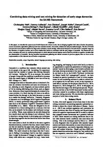
The case study described in this section is a beam structure that was presented in [15]. It is used to illustrate the methodology described in Section 2.2. Although this study focuses on bridge structures, it can be applied to other structures and in other domains. The procedure for generating models from modeling assumptions is given in [15]. In this particular example, six parameters consisting of position and magnitude of three loads have been chosen. After running the procedure described in Section 3, the number of clusters is chosen to be three in this case. The results are shown in Table 3. It can be seen that the maximum value for the score function is reached with three clusters and a local maximum can be observed with six clusters. This effect can also be seen on the right part of Figure 1 where the three clusters could be divided into two to obtain six clusters. Furthermore, BCD and WCD are always increasing. This is due to the fact that at maximum there could be one cluster for each point. Once the number of clusters is fixed, the procedure outlined in Table 1 is followed. To judge the improvement of the methodology with respect to the standard k-means algorithm, the two techniques are compared. Figure 1 shows
Clusters BCD WCD SF 2 78.43 1.65 47.67 3 127.70 1.96 65.22 4 147.59 2.34 63.09 5 166.35 2.66 62.68 6 181.26 2.89 62.80 7 192.11 3.12 61.60 8 202.83 3.31 61.39 Table 3. Comparison of values for between class distance (BCD), within class distance (WCD) and score function (SF) for various numbers of clusters.
the improvement in a visualization point of view. The left part of Figure 1 corresponds to standard k-means whereas the right part is the result of the methodology described in this paper. It is easy to see that our methodology is better able to present results visually.
Fig. 1. Visual comparison of standard k-means (left) with respect to the proposed methodology (right). Every point represents a model and belongs to one of the three possible clusters (+, O or 4).
This methodology has a number of limitations. Firstly, results of data mining have to be interpreted carefully. The user thus has an important role in ensuring that the methodology is successful. Secondly, even if the methodology is well applied, results are not necessary the most appropriate. For example, data might be noisy (poor sensor precision), or may have missing values (low sensor quality) or may be missing useful information (bad sensor configuration) and this may preclude obtaining useful results. An example of challenges associated with applying data mining to system identification is given below. Assume that, after applying data-mining methodology, three clusters of models are obtained. The methodology alone is not able
to interpret these clusters. Suppose that two clusters group similar information. Although the clustering algorithm has generated three clusters, only the user is able to identify that there are only two clusters that have physical meaning. Therefore, data mining is only able to suggest possible additional knowledge. The process of acquiring knowledge that is of practical use for decision-support is left for the engineer.
5
Conclusions
A methodology that combines PCA and k-means for studying the solution space of models obtained during system identification is presented in this paper. The conclusions are as follows: • Combining the data mining techniques, PCA and k-means, helps improve visualization of data • Evaluation of results obtained through clustering is difficult The metric that has been developed in this work helps in the evaluation • Application of data mining to complex tasks such as system identification requires an expert user Future work involves the use of more complex data mining methods to obtain other ways for separating and clustering models. Furthermore, better visualization of solution spaces needs to be addressed in order to improve engineer/computer interaction. Finally, strategies for models containing a varying number of parameters are under development.
Acknowledgments This research is funded by the Swiss National Science Foundation through grant no 200020-109257. The authors recognize Dr. Fleuret for several fruitful discussions on data mining techniques. The two anonymous reviewers are acknowledged for their propositions which have modified the direction of the paper.
References 1. Alonso C., Rodriguez J.J. and Pulido B. Enhancing Consistency based Diagnosis with Machine Learning Techniques. LNCS, Vol. 3040, 2004, pp. 312-321. 2. Chan Z.S.H., Collins L. and Kasabov N. An efficient greedy k-means algorithm for global gene trajectory clustering. Exp. Sys. with Appl., 30 (1), 2006, pp. 137-141. 3. Ding C. and He X. K-means clustering via principal component analysis. Proceedings of the 21st International Conference on Machine Learning, 2004. 4. Hand D., Mannila H. and Smyth P. Principles of Data Mining. MIT Press, 2001, 546p. 5. Jolliffe I.T. Principal Component Analysis. Statistics Series, Springer-Verlag, 1986, 271p.
6. Ljung L. System Identification - Theory For the User. Prentice Hall, 1999, 609p. 7. Melhem H.G. and Cheng Y. Prediction of Remaining Service Life of Bridge Decks Using Machine Learning. J. Comp. in Civ. Eng., 17 (1), 2003, pp. 1-9. 8. Nguyen H.H. and Chan C.W. Applications of data analysis techniques for oil production prediction. Art. Int. in Eng., Vol 13, 1999, pp. 257-272. 9. Ordonez C. Integrating k-means clustering with a relational DBMS using SQL. IEEE Trans. on Know. and Data Eng., 18 (2), 2006, pp. 188-201. 10. Pan X., Ye X. and Zhang S. A hybrid method for robust car plate character recognition. Eng. Appl. of Art. Int., 18 (8), 2005, pp. 963-972. 11. Picone J. Duration in context clustering for speech recognition. Speech Com., 9 (2), 1990, pp. 119-128. 12. Raphael B. and Smith I.F.C. Fundamentals of Computer-Aided Engineering. John Wiley, 2003, 306p. 13. Reich Y. and Barai S.V. Evaluating machine learning models for engineering problems. Art. Int. in Eng., Vol 13, 1999, pp. 257-272. 14. Robert-Nicoud Y., Raphael B. and Smith I.F.C. Improving the reliability of system identification. Next Gen. Int. Sys. in Eng., No 199, VDI Verlag, 2004, pp. 100-109. 15. Saitta S., Raphael B. and Smith I.F.C. Data mining techniques for improving the reliability of system identification. Adv. Eng. Inf., 19 (4), 2005, pp. 289-298. 16. Shirazi Kia S., Noroozi S., Carse B. and Vinney J. Application of Data Mining Techniques in Predicting the Behaviour of Composite Joints. Eighth AICC, 2005, Paper 18, CD-ROM. 17. Tan P.-N., Steinbach M. and Kumar V. Introduction to Data Mining. Addison Wesley, 2006, 769p. 18. Webb A. Statistical Pattern Recognition. Wiley, 2002, 496p. 19. Xu L.J., Yan Y., Cornwell S. and Riley G. Online fuel tracking by combining principal component analysis and neural network techniques. IEEE Trans. on Inst. and Meas., 54 (4), 2005, pp. 1640-1645. 20. Yan L., Fraser M., Oliver K., Elgamal A., Conte J.P. and Fountain T. Traffic Pattern Recognition using an Active Learning Neural Network and Principal Components Analysis. Eighth AICC, 2005, Paper 48, CD-ROM. 21. Yun C.-B., Yi J.-H. and Bahng E.Y. Joint damage assessment of framed structures using a neural networks technique. Eng. Struct., Vol 23, 2001, pp. 425-435.