Combining Simulation and Formal Methods for System-Level Performance Analysis Simon K¨unzli ∗ ETH Z¨urich
Francesco Poletti Universit`a di Bologna
Luca Benini Universit`a di Bologna
Lothar Thiele ETH Z¨urich
[email protected]
[email protected]
[email protected]
[email protected]
Abstract Recent research on performance analysis for embedded systems shows a trend to formal compositional models and methods. These compositional methods can be used to determine the performance of embedded systems by composing formal analytical models of the individual components. In case there exist no formal component models with the required precision, simulation-based approaches are used for system-level performance analysis. The often high runtimes of simulation runs lead to the new approach described in this paper: Analytical methods are combined with simulation-based approaches to speed up simulation. We describe how the simulation models can be coupled with the formal analysis framework, specify the interfaces needed for such a combination and show the applicability of the approach using a case study.
1
Introduction
System-level performance evaluation of heterogeneous embedded systems becomes increasingly important the larger these systems are designed. Recently, many processing devices for embedded systems are designed as systemson-chip (SoC) [23]. Using this design paradigm, a complete system consisting of computing, storage and communication resources is integrated on the same chip. Such a system may consist of several IP cores and dedicated hardware, as the Cell processor announced recently by Sony, IBM and Toshiba [15]. To shorten the design times, predefined and verified cores are used for newly designed systems [2]. Using cores, the designers can concentrate on overall system design instead of working on the individual components. Performance evaluation of embedded systems can be broadly divided in two main areas: simulation-based approaches and formal methods. The trend for simulationbased performance analysis goes to full system simulation [7, 19, 21]. ∗ Simon K¨ unzli has been supported by the Swiss Innovation and Promotion Agency (CTI/KTI) under project number KTI 5500.2
3-9810801-0-6/DATE06 © 2006 EDAA
Formal methods for performance evaluation are emerging that enable the analysis of whole systems using holistic [16] and compositional approaches. In particular, the system can be analyzed using models of the individual components that can be later composed to capture the complete system [17, 10]. Actually, there is no sharp division into simulation-based approaches and formal methods for system-level analysis. There exist approaches that abstract communication internals in system simulation and use transaction-level modeling in SystemC [4]. Lahiri et al. present a combined approach to communication analysis which uses simulation for parameter extraction and then a formal method for fast performance analysis [11]. Bobrek et al. also combine simulation with an analytical method in [3], with focus on the analysis of shared resource contention. They simulate parallel execution of threads and record accesses to shared resources, while a formal analysis model is then used to determine the adjustment of the timing caused by the shared resource contention. The long run-times for simulation-based approaches are a drawback for this class of performance evaluation methods. Our new method reduces the run-time of an evaluation and reflects the idea of components. In analogy to component-based design where existing IP blocks are combined to form a SoC, our method allows the designer to reuse existing analysis models for components – be it a simulation model or a formal model – for the individual components and compose them to form the complete system model. The existing component models may result from previous designs or may be delivered by IP vendors. Performance evaluation is then conducted using these trusted models of the components. The approach presented in [3] is orthogonal to our approach, as it uses a hybrid approach for in-component analysis, and could be used in addition to further decrease simulation time. The contribution of this paper is the definition of a new hybrid approach for performance evaluation. In particular, the definition of the needed interfaces is provided, they were implemented, and the new method is used in a case study.
2 2.1
Methods for Performance Evaluation SystemC-based virtual platform
MPARM is a multi-processor cycle accurate virtual platform based on SystemC [13]. Its purpose is the system-level analysis of design tradeoffs in the usage of different processors, interconnects, memory hierarchies and other devices. Processor cores are modeled by means of an adapted version of a GPL-licensed ARM Instruction Set Simulator (ISS) called SWARM [20] and written in C++. Since all of the hardware devices mentioned above, including the interconnection layer, are coded in SystemC, we embedded the ISS into a SystemC wrapper. The platform instantiates several memory devices, which can be used as private or shared memories (cf. Fig. 1). Their latency can be configured to explore interconnection performance under several conditions. We ported the RTEMS [18] and uclinux [22] operating system to our platform. Private Memory
Private Memory
Shared Memory
Semaphore Slave
Slave Port
Slave Port
Slave Port
Slave Port
Communication Architecture
Master Port Snoop Port
Master Port
ARM7
Snoop Port
ARM7
2.3 Slave Port
Interrupt Slave
Figure 1. MPARM platform architecture.
2.2
Real-Time Calculus
In [5], Chakraborty et al. present Real-Time Calculus (RTC), a system-level performance analysis method for embedded systems. It is based on arrival curves and service curves, a tool to characterize workload and processing capabilities, respectively. For a given event stream, let R(t) denote the number of events that arrive in the time interval [0, t]. The upper arrival curve, denoted by αu gives an upper bound on the number of events in any interval. Similarly, a lower bound on the number of events arriving is given by a lower arrival curve αl . R, αu and αl are related by the following equations: αl (∆)
=
min{R(∆ + λ) − R(λ)}
(1)
αu (∆)
=
max{R(∆ + λ) − R(λ)}
(2)
λ≥0
λ≥0
window of size ∆ and keep the maximum and minimum number of events that can be seen in the window. The maximum leads to the upper arrival curve, the minimum to the lower curve. The arrival curves describe timing properties of a class of event streams, for example the average rate, burstiness, long-term and short-term behavior. The workload characterizations for simulation and RTC can hence be based on the same type of data, which makes RTC suitable for a combination with a simulation-based approach. The conversion of the event models from RTC to simulation and vice versa is described in Sec. 3. Using RTC, it is possible to determine worst-case bounds on on-chip memory requirements, overall throughput and delay, if the following information is available: (1) the arrival curves capturing the workload, (2) a task graph describing the structure of the application, (3) a mapping of the tasks to processing units and (4) a scheduling policy on these resources. Furthermore, it is possible to give bounds on the utilization of the processing elements in the system and to get a description of the output event stream after being processed in the form of an arrival curve. The method supports the analysis of computation and communication tasks and several scheduling policies such as fixed-priority or TDMA.
The upper and lower arrival curves for an event stream can be computed from simulation traces. For all possible intervals ∆ we browse through the trace using a sliding
Comparison of the Approaches
Before we can combine the two approaches, we have to validate whether the results of a formal method for performance analysis match those of a detailed simulation. There exist studies comparing the different approaches and discussing their limitations. But the comparison results in [8, 6] are obtained for network processors and therefore not suitable for the platform and application domain used here. The approach taken to compare the results is depicted in Fig. 2. We first defined an input sequence for the simulation (1). From this sequence with which the first stage of the matrix multiplication pipeline is triggered, we computed the upper and lower arrival curves which are used for the formal analysis method (2). We then performed the simulation of the system and the analysis (3), and calculated the arrival curve from the simulation output (4) in order to be able to compare the two approaches (5). We perform the comparison based on arrival curves, because they give a compact characterization of the processed event streams and we can determine properties of the event streams, such as delay, burstiness, or timing behavior directly from these curves. In Fig. 3, we give the results obtained for a multistage matrix multiplication application. It is organized as a pipeline, with 8 consecutive tasks of different worst-case execution times to be executed for the application to complete. The execution platform used for the comparison consists of 4 ARM7 processors connected with a AMBA bus. The data transfer between the tasks is done using a shared
2
Simulation Input Events
Arrival Curve Calculation
Simulation on MPARM Platform
Simulation Output Events
3
Input Arrival Curves
3
Analysis using Real-Time Calculus
Arrival Curve Calculation
Output Arrival Curves
2
comparison
5
7
1
3
5
7
3
4
6
CPU 1
CPU 2
CPU 3
0
2
4
6
CPU 0
CPU 1
CPU 2
CPU 3
1
CPU 0
5
Scenario 1
[# events]
Figure 2. Procedure for the comparison of the analytical approach and the simulation.
Run-Time [s] 0.965 43–321 0.984 42–384
Table 1. Run-times of evaluation methods for the 2 different scenarios.
0
4
Method RTC Simulation RTC Simulation
Sc. 1 1 2 2
Scenario 2
Scenario 1
10 8 6 4
3
Interfaces between Simulation and Formal Method
In this section we will introduce the interfaces needed to combine system simulators with formal analysis models for a hybrid analysis. Because formal analysis methods
0
5
10
15
6
8
Simulation
0 0
20 [ms] 25
Real-Time Calculus Scenarios 1 & 2
10
[# events]
8
2
Scenario 2
6 4
5
10
15
20 [ms] 25
Simulation Scenarios 1 & 2
10
[# events]
0
8
Scenario 2
6 4
2 0
Real-Time Calculus
4 Simulation
2
memory attached to the bus. We modeled two scenarios with a different mapping of the tasks to the resources as shown in Fig. 3(top). The diagrams in Fig. 3(middle) depict the output arrival curves for the two scenarios. The curves show on the one hand the arrival curves describing the worst-case output traffic as predicted by RTC and on the other hand they give the arrival curves describing the output traffic generated by the simulation. As the modular performance analysis method is based on worst-case analysis, the curves resulting from the analytical method lie outside of the curves based on simulation (cf. Sec. 2.1), as expected. This can be interpreted as follows: In case of simulation for scenario 1, the smallest time interval where there are 4 events is 6 ms, the largest interval is 9.9 ms for the used trace. For RTC, the smallest interval is 5 ms, the largest interval is 10 ms. Fig. 3(bottom) shows that the trends for the output traffic pattern for the two scenarios that are shown by both RTC (left) and the simulation (right) match well. This result allows us to claim the ability of RTC to correctly predict the behavior of a component. The run-times of the two approaches for the example application are shown in Table 1. RTC uses less than a second to complete whereas the corresponding simulation framework takes between 40 seconds an around 6 minutes to complete dependent on the waiting time between consecutive activations of the matrix multiplication. This increase in simulation speed comes at the cost of a pessimistic prediction of task execution, and therefore resource consumption.
Scenario 2
10
Real-Time Calculus
[# events]
1
0
5
10
15
20
Scenario 1
2
Scenario 1 [ms]
25
0
0
5
10
15
20 [ms] 25
Figure 3. top: Mapping for the two scenarios. middle: Comparison between arrival curves computed from simulation and with RTC bottom: Comparison between RTC (left) and simulation (right).
work for non-functional property analysis only, the hybrid approach can also cover only these aspects and functional analysis has to be performed using a functional simulator. S/F-converter
F/S-converter
T1
T2
simulation
formal analysis
T3
T4 simulation
Figure 4. The task chain for hybrid approach with resource-independent components.
Figure 4 gives an example system model for the hybrid approach. We can identify two problems, (i.) the interface from simulation to formal models and (ii.) the interface
from formal analysis models to simulation (cf. Fig. 4). In order to introduce these interfaces more formally, we define what we understand by an event trace and an event class. Definition 1 Event trace. An event trace is a sequence of events (ei , ti ), where ei denotes the event data and ti the time stamp at which the event data ei is available to the application. The set of all events is denoted as E, i.e. (ei , ti ) ∈ E. Definition 2 Event class. An event class is formed by events that have to be processed in the same way by an application. Events belonging to the same event class take the same path through an application task graph. If (ej , tj ) ∈ Ei , then event (ej , tj ) belongs to an event class Ei .
3.1
non-functional property analysis
F/S-converter A/S-converter arrival curve based event stream generator
event data
event data …
data extractor
simulation trace
time stamps data synchronizer event data
event data
event data
…
event data
functional simulator
Figure 6. Interface between simulator and a formal analysis method: the F/S-converter.
S/F-Converter
The conversion of event streams from the simulation subsystem into an event model for the formal analysis method appears to be much simpler than the reverse direction. Once the simulation of a component has finished, we can analyze the output event traces of the form (e1 , t1 ), (e2 , t2 ), ..., (ei , ti ), (ei+1 , ti+1 ), ... . First, we have to classify the events in the event trace and annotate them with the event class they belong to. In the next step we can derive the upper and lower event arrival curve that represent each event class Ek with: R(t) = |{(ei , ti ) ∈ Ek : ti ≤ t}| From R(t), we can then compute αl , αu with equations (1) and (2) in Sec. 2.2. S/F-converter S/A-converter time classifier stamps trace analyzer
simulation trace
event data
event data
…
event data
event data
data collector
non-functional property analysis event data
event data …
functional simulator
Figure 5. Interface between formal analysis method and simulator: the S/F-converter. The event classification and the arrival curve calculation are performed by the classifier and the trace analyzer shown in Fig. 5. The event data items ei are sorted according to the event classes by the data collector. The output from the trace analyzer, the arrival curves describing the timing of the event stream are then passed to the formal analysis method, whereas the event data collection is passed to the functional simulator for further processing.
3.2
with RTC as formal method and the MPARM simulation framework written in SystemC [9], the problem of designing an F/S-converter (as shown in Fig. 6) can be seen as designing a SystemC module, which generates events according to the arrival curve that was obtained using RTC.
F/S-Converter
An F/S-converter transforms event models that result from the formal analysis method into event traces used for the simulation. This conversion tool from the formal method to simulation is more involved than the S/Fconverter introduced in the previous section. In our setup,
The generated trace of time stamps has to fulfill a set of requirements: First of all, a generated trace must not violate neither the upper nor the lower arrival curve received from the formal analysis. Second, we would like the generated traces to represent a bad-case, bursty behavior, as arrival curves are used for worst-case analysis. Nevertheless, the generated trace should also be representative for the arrival curve as a whole. In this sense, the generated trace should show “fractal” behavior [12], i.e. in a short observation interval, the trace should be as bursty as allowed by the upper and the lower arrival curve in a short time interval — whereas for a larger observation interval, the trace should represent the whole upper and lower arrival curves. The main idea underlying the proposed event trace generation algorithm is to use an ON/OFF traffic source (see e.g. [1]). In contrast to standard ON/OFF models, if our event generator is in the ON state, we generate events as soon as we are allowed by the upper curve. Similarly, if in the OFF state we generate an event only if the lower arrival curve would be violated otherwise. The basic event trace generation algorithm consists of three main steps: 1. determine time stamp T at which to switch state 2. generate events according to state while time t < T 3. switch state and go to step 1. The time t is set to 0 after a state switch and denotes the time spent in a state. The switch time T is determined using a Weibull-distribution to best reflect the desired behavior [1]. Additional information needed for the simulator, such as the event type, which may not be included in the analytical description of the event stream, has to be passed to the data extractor. In the data synchronizer the event time stamps and the corresponding event data are synchronized and used to trigger the simulator. In the case study presented in the next section, we use a traffic generator written as a module in SystemC to feed the data into the simulator, at times
determined by an event trace generator based on the arrival curves obtained by the formal analysis method. The traffic generator module is described in more detail in [14].
3.3
Benefits of hybrid approach
The hybrid approach presented in this paper can be used to analyze applications that consist of task chains. It is possible to cut this chain into segments of the chain that are executed on independent hardware resources. These segments can then be either analyzed using the formal method, and if not applicable analyzed using a simulator (cf. Fig. 4). Using the hybrid approach, we can lower the overall execution time compared to simulation because of two reasons: (1) The run-time of a single evaluation for the hybrid approach is significantly smaller than with simulation, because we replace individual simulator components by formal models. (2) The F/S-converter constructs short, representative traces for simulation from the formal model. As a consequence, less simulation runs are needed for a good coverage. Assume that for the task chain given in Fig. 4, we have to perform n pure simulations to well cover all possible load scenarios. For the hybrid approach, we still have to perform n simulation runs for the components before the S/F-converter, the converter then aggregates the n simulation traces to a single pair of arrival curves, representing the n traces. The analysis has to be performed only once and the output of the formal analysis, a trace generated by the F/Sconverter has also to be simulated only once, as the trace is generated based on the aggregation of all input traces. The analysis method as it is presented in this paper can handle feed-forward data flow graphs, without feedback loops across the borders between the different analysis methods. Further, data splits or joins are restricted to occur in simulation components due to limitations of the formal analysis method used. These usage restrictions shall be tackled in future work.
4
Case study
For the case study, we analyzed a GSM audio encoder application. The tasks graph of the application consists of a chain of 21 consecutive tasks. It receives sequences of frames as input that have to be encoded before being transmitted. These input frames are guaranteed to respect certain best/worst case bounds, while the encoded sequences have also to respect bounds in order to guarantee a good communication. We first specified the load traffic that should be supported by the GSM encoder application by means of an arrival curve describing upper and lower bounds on the arrival of packets to be processed by the encoder. After a static profiling of the application we partitioned the task chain to be executed on two processors to obtain a balanced system. The two processors are connected with a AMBA-bus and communicate over a FIFO-queue located in a shared memory attached to the bus.
We performed 3 experiments for the analysis of the system: (1) We used only RTC, (2) we used the hybrid approach presented in this paper, and (3) we performed a full system simulation. For all the 3 experiments we used the same input load, either event traces (for the simulation) or the corresponding input arrival curve (for the hybrid approach and the formal analysis). The input load specifies the arrival of frames to be encoded. For the hybrid approach, we partitioned the system as shown in Fig. 7(left). As described in Sec. 3.2, we use an F/S-converter to interface between RTC and the simulator. We replaced one ARM7 processor by its formal model and integrated a traffic generator into the MPARM simulation framework. The traffic generator puts the intermediate data collected from a functional simulation of the GSM encoder application into the FIFO-queue. The curves presented in Fig. 7(middle) show the output arrival curves for the 3 experiments. The curves give upper and lower bounds on the number of audio frames that are finished processing in any time interval. The upper and lower output curve were calculated for exp. 1 using RTC, and obtained from the output simulation traces in case of the hybrid approach (exp. 2) and the simulation (exp. 3) using the same procedure as described in Sec. 3.1. The outermost curves give the upper and lower arrival curve calculated with RTC. RTC is a method for worst-case analysis, i.e. the other curves have to lie within the bounds obtained with this method. The curves for the hybrid approach lie between the curves for RTC and the simulation curves. This behavior of the hybrid approach is also expected, as the first part of the analysis was performed using a worst-case analysis method, and the synthetic trace used as stimulation for the second part is based on the worst-case arrival curves. We now look at the fill level of the intermediate buffer between the two processors. In case of RTC we predict that the buffer fill level is at most 5 frames waiting to be processed. For the pure simulation, the maximum buffer fill level varies between 1 and 4. Dependent on the simulation trace used, we derive different design values for the queue size needed (cf. Fig. 7(right)). In contrast, for the hybrid analysis run, we can see that the buffer fill level is at most 4 frames waiting in the queue with only a single simulation. Table 2 gives the run-times for the three different experiments. The times are given for a single evaluation run. The hybrid approach allows to speed up the simulation by a factor of 1.73 for our example. This is a significant improvement, because we still simulate more than half of the system (cf. Fig. 7(left)). Using the new method described in this paper, we could (1) speed up the simulation for a single evaluation run and (2) lower the number of simulation runs needed for a complete system evaluation.
T5
T1
[# events]
12
15 tasks
6 tasks
T6
T7
T8
hybrid analysis 10
T21
Real-Time Calculus
5 4 3 2 1 0
Simulation Trace 1
5 4 3 2 1 0
Simulation Trace 2
8
CPU0
CPU1 6
simulation
memory 4
RTC
Simulation F/S-converter
output arrival curves
2
0
0
200
400
600
800
1000
1200
1400
1600
1800
[ms]
2000
5 4 3 2 1 0
200 ms
200 ms
Hybrid Approach
200 ms
Figure 7. left: System model for exp. 2. middle: Output arrival curves for the 3 exp. right: Buffer fill levels over time for 2 simulation runs and the hybrid approach.
Exp. 1 2 3
Method RTC Hybrid Simulation
Run-Time [s] 0.273 292 508
Table 2. Run-times of evaluation methods for a single run of the GSM encoder.
5
Conclusion
In this paper, we presented a hybrid approach for systemlevel performance evaluation of embedded systems that combines formal analysis methods with a simulation framework. We defined the interfaces needed for this combination and showed the applicability using a case study. In addition to the benefits discussed in this paper, the approach also allows us to shorten the development times for the evaluation system model. This is due to the fact that not all components have to be written as SystemC simulation models, but analytical components can be used. In future, we would like to apply the hybrid approach to analyze larger systems. Furthermore, we believe that for the approach presented in this paper there are more and more application scenarios, as for the design of embedded systems an increasing number of reusable components exist and the systems tend to become more and more complex.
Acknowledgments The work presented in this paper has been funded in parts through the European Network of Excellence ARTIST2.
References [1] P. Barford and M. Crovella. Generating representative web workloads for network and server performance evaluation. In Proc. SIGMETRICS, pages 151–160. ACM Press, 1998. [2] R. Bergamaschi et al. Automating the design of SoCs using cores. IEEE Design and Test of Computers, 18(5):32–45, 2001. [3] A. Bobrek, J. J. Pieper, J. E. Nelson, J. M. Paul, and D. E. Thomas. Modeling shared resource contention using a hybrid simulation/analytical approach. In Proc. DATE’04, pages 1144–1149. IEEE Computer Society, 2004. [4] L. Cai and D. Gajski. Transaction level modeling: an overview. In Proc. CODES+ISSS, pages 19–24, New York, NY, USA, 2003. ACM Press.
[5] S. Chakraborty, S. K¨unzli, and L. Thiele. A general framework for analysing system properties in platform-based embedded system designs. In Proc. DATE, pages 190–195, March 2003. [6] S. Chakraborty, S. K¨unzli, L. Thiele, A. Herkersdorf, and P. Sagmeister. Performance evaluation of network processor architectures: Combining simulation with analytical estimation. Computer Networks, 41(5):641–665, April 2003. [7] ConvergenSC the Advanced System Designer, Coware. http://www.coware.com/products/. ./convergensc techoverview.php. [8] M. Gries, C. Kulkarni, C. Sauer, and K. Keutzer. Comparing analytical modeling with simulation for network processors: A case study. In Proc. DATE, March 2003. [9] T. Gr¨otker, S. Liao, G. Martin, and S. Swan. System Design with SystemC. Kluwer Academic, Boston, May 2002. [10] R. Henia, A. Hamann, M. Jersak, R. Racu, K. Richter, and R. Ernst. System level performance analysis – the SymTA/S approach. IEE Proc. - CDT, 152(02), March 2005. [11] K. Lahiri, A. Raghunathan, and S. Dey. Design space exploration for optimizing on-chip communication architectures. IEEE Trans. on Computer-Aided Design of Integrated Circuits and Systems, 23(6), 2004. [12] W. E. Leland, M. S. Taqqu, W. Willinger, and D. V. Wilson. On the self-similar nature of Ethernet traffic. In Proc. ACM SIGCOMM, pages 183–193, 1993. [13] M. Loghi, F. Angiolini, D. Bertozzi, L. Benini, and R. Zafalon. Analyzing on-chip communication in a MPSoC environment. In Proc. DATE’04, pages 752–757, 2004. [14] S. Mahadevan, F. Angiolini, M. Storgaard, R. G. Olsen, J. Sparso, and J. Madsen. A network traffic generator model for fast networkon-chip simulation. In Proc. DATE, pages 780–785. IEEE Computer Society, 2005. [15] D. Pham et al. The design and implementation of a first-generation CELL processor. In Proc. ISSCC, February 2005. [16] P. Pop, P. Eles, and Z. Peng. Analysis and optimization of heterogeneous multiprocessor SoC. IEE Proc. - CDT, 152(02), March 2005. [17] K. Richter, M. Jersak, and R. Ernst. A formal approach to MPSoC performance verification. Computer, 36(4):60–67, 2003. [18] RTEMS home page. http://www.rtems.com. [19] Seamless Hardware/Software Co-Verification, Mentor Graphics. http://www.mentor.com/seamless/. [20] Software ARM. http://www.cl.cam.ac.uk/. ./users/mwd24/phd/swarm.html. [21] Synopsys System Studio, Synopsys. http://www.synopsys.com/products/. ./cocentric studio/cocentric studio.html. [22] uClinux, Embedded Linux Microcontroller Project. http://www.uclinux.org/. [23] W. Wolf. Computers as components: principles of embedded computing system design. Morgan Kaufmann Publishers Inc., San Francisco, CA, USA, 2001.