Community Evolution Prediction in Dynamic Social Networks

Community Evolution Prediction in Dynamic Social Networks Mansoureh Takaffoli, Reihaneh Rabbany, Osmar R. Za¨ıane Department of Computing Science, University of Alberta, Edmonton, Alberta, Canada T6G 2E8 Email:{takaffol, rabbanyk, zaiane}@ualberta.ca Abstract— Finding patterns of interaction and predicting the future structure of networks has many important applications, such as recommendation systems and customer targeting. Community structure of social networks may undergo different temporal events and transitions. In this paper, we propose a framework to predict the occurrence of different events and transition for communities in dynamic social networks. Our framework incorporates key features related to a community – its structure, history, and influential members, and automatically detects the most predictive features for each event and transition. Our experiments on real world datasets confirms that the evolution of communities can be predicted with a very high accuracy, while we further observe that the most significant features vary for the predictability of each event and transition.

I.

I NTRODUCTION AND BACKGROUND

A social network shows the structure of relationships between individuals, where the relationships are usually defined based on some type of interaction, hence are intrinsically temporal and changing over time; examples are friendships between people, co-authorships between scholars, email interactions between employees within an organization, etc. Modeling a dynamic network enables the study of its structure over time, the detection of how the network evolves, and ultimately the prediction of the future structure of the network. Finding patterns of interaction and predicting the future structure of networks has many applications, such as in viral marketing [1], revenue maximization [2], and social influence [3]. It can help decision makers setup profitable marketing strategies in advance. However, very little work has been done on why dynamic networks experience specific evolution transitions. Most of the previous research in this area focus on either predicting the macroscopic graph structure, or the microscopic properties from the point of view of a single node or edge. In this paper, we consider predicting the trend of one mesoscopic structure, called community. The community consists of a group of nodes that are relatively densely connected to each other but sparsely connected to other dense groups in the network. Analysis of the evolution of communities is related to important social phenomena such as homophily [4] and influence [5]. In social networks, communities can be either explicit or implicit. Explicit communities are built independently from their members and are based on a set of rules. In this case, people mostly join communities after the formation of the communities. Employees of a company or students participating in a course are examples of two explicit communities. On the other hand, the formation of implicit communities

heavily depends on their members and connections. In this paper, we mainly focus on implicit communities and the setting where at any given time, an individual can belong to only one community. In this setting, which is called non-overlapping communities or hard-partitioning, a community serves as the main engagement platform for the individual. An individual can move from one community and join another one, while the amount of interactions between members of a community also changes over time. Thus, a community experiences different events and transitions during its life. In this paper, we propose a machine learning model to accurately predict the next event and transition of a community, based on the relevant structural and temporal properties. The first contribution of our model is leveraging the relation between the behavior of individuals and the future of their communities. Members of a community play an important role in attracting new members and generally shaping the future of their community. This fact is however overlooked by all previous works. Our models further assume that individuals who are more likely to undertake actions in their communities, are more influential in the future trend of their community, and therefore are principal factors in the predictive process. For instance, in marketing strategy, considering the impact of individuals on their communities is necessary for targeting the right consumers to direct advertisement, and to maximize the expectation of the total profit [6]. Moreover, unlike previous works that only consider one aspect of the communities (i.e. size, age, or event), our models provide a complete predictive process for any transition and event that a community may undergo, and at the same time, identify the most prominent features for each community transition and event. The last important distinction of our model is that our events and transitions do not have to taken place in consecutive snapshots. A community may not necessarily be observed at consecutive snapshots, while it may be missing from one or more intermediate steps. Hence, our model predicts the next stage of a community either in the exact next snapshot or any later snapshot. Before describing our method, we need to first review few notations from [7]. A dynamic social network is modelled as a sequence of graphs {G1 , G2 , ..., Gn }, where Gi = (Vi , Ei ) denotes the graph at snapshot i, which contains Vi individuals and Ei interactions. The set Ci = {Ci1 , Ci2 , ..., Cini } represents ni communities detected at snapshot i, where each community Cip ∈ Ci is also represented by a graph (Vip , Eip ). We consider two communities from different snapshots similar if the ratio of their mutual members exceeds a threshold, more formally:

Community Similarity: Similarity of communities Cip and Cjq , detected at snapshot i and j 6= i, is measured as: ( |Vip ∩Vjq | |Vip ∩Vjq | if max(|V ≥k p q p p q max(|V |,|V |) |,|Vjq |) sim(Ci , Cj ) = i j i 0 otherwise (1) Based on this notion of similarity, changes that occur for a community are defined as: form, dissolve, split, merge, or survive. Note that, the events and transitions formulation proposed in [7], track the changes of communities over the entire observation time, rather than only between two consecutive snapshots. Moreover, the instances of the same community at different time-frames are considered as one meta community, formally defined as: Meta Community: Given a set of snapshots 1, 2 . . . n, a meta community is a sequence of communities M = {Ctp11 , Ctp22 , ..., Ctpmm } such that (a) (b)

1 ≤ t1 < t2 < ... < tm ≤ n, p ∀ ti , t1 < ti ≤ tm ∃ tj < ti : sim(Ctjj , Ctpii ) > 0 II.

P ROBLEM F ORMULATION

In predicting the trend of a community using predictive models, a response variable is a property related to community which can quantify a particular change in a community over time. A feature is any property that can influence one of the response variables. Thus, the first step is to select appropriate features from the properties related to entities and communities, as well as deciding on the response variables. Then, we can model the relationship between each response variable and one or more features, which can be used later to predict the most probable changes that may occur for a community. A. Community Transitions and Events as Response Variables In the case of implicit communities, where the formation of communities heavily depends on their members and connections, an entity may leave its current community and join another community, due to the shifts of their interests or due to certain external events. Thus, when a community survives into next snapshot, it may also experience different transitions. It may expand if the number of its members increases, or shrinks if the number of its members decreases. Moreover, members of a survived community may change their engagement level, making the community more cohesive, or loose. Based on these transitions and the events [7], we quantify the changes that may occur for a community as follows: survive{true, false}, merge{true, false}, split{true, false}, size{expand, shrink}, and cohesion{cohesive, loose}. All these events and transitions are binary which constitute the response variables in our predictive model. Since size and cohesion transitions only defined for a survival community, we propose a multistage cascading technique to detect these two transitions. First, we predict the survival, then the detection of these transitions is followed. These response variables are not mutually exclusive and may occur together at the same time, where different features may trigger them. Hence, we learn separate models to predict each of them.

Here, we consider the cohesion of a community as how closely its members interact with each other relative to outside of the community. More formally: Cohesion: Cohesion of a community Cip at snapshot i is: cohesion(Cip ) =

2|Eip | p |Vi |(|Vip |−1) |OEip | p |Vi |(|Vi |−|Vip |)

=

2|Eip |(|Vi | − |Vip |) |OEip |(|Vip | − 1)

(2)

where |OEip | is the set of outer edges of community Cip . B. Properties of Community as Features To predict the next stage of a community, we consider three main classes of features: properties of its influential members, properties of the community itself, and temporal changes of these properties. These features are summarized in Table I, and are explained in detail in the following. 1) Properties of its influential members: The evolution of network is usually analyzed by considering all members and their properties. However, communities are often led by a smaller set of individuals, who have considerable influence over other members, and shape the fate of their community. To identify the influential nodes in a community we use the role leader defined in the role mining framework proposed by Abnar [8]. The leaders of a community are defined as the outstanding individuals in terms of centrality or importance in that community. To detect the leaders of a community, the probability distribution function (pdf) of closeness centrality scores for all the nodes in each community is computed. As Abnar [8] found out, this pdf is close to a normal distribution, and therefore, the upper threshold of µ + 2σ 1 can be used to distinguish the leaders. For these detected leaders, we consider two structural features, i.e. their degree and closeness centrality scores. Since a community may have more than one leader, we take the average degree and closeness centrality scores of the detected leaders. We also consider the ratio of the leaders to the community size as a separate feature for the community. Similarly, we consider the ratio of outermosts in a community as another feature. Where Outermosts are defined as the small set of least significant individuals in the community [8] 2 . 2) Structural properties of the community itself: To quantify the structural properties of a community we consider its size (number of nodes), cohesion (Equation 2), density, and clustering coefficient. The density, and clustering coefficient of a community Cip are defined as: Density: The ratio of edges to the maximum possible edges: density(Cip ) =

2|Eip | |Vip |(|Vip | − 1)

(3)

Clustering coefficient: The ratio of edges between neighbours of a nodes to the maximum possible edges between 1 according to the properties of a normal distribution, almost 95% of the population lies in the interval [µ − 2σ, µ + 2σ], where µ and σ are mean and standard deviation of this distribution. 2 Similar to leaders, from the pdf of the closeness centrality scores, we use µ − 2σ as the lower threshold to identify outermosts

them. More formally, clustering coefficient of node v is: clustering-coeff(v) =

|{(u, w)|(v, u), (v, w), (u, w) ∈ E}| |{(u, w)|(v, u), (v, w) ∈ E}|

The clustering coefficient of a community is then defined as the mean of clustering coefficient of all its members: P v∈Cip clustering-coeff(v) p clustering-coeff(Ci ) = (4) |Cip | Similar to the clustering coefficient, we also consider the average and variance of the centrality scores of all members as separate features. 3) Temporal changes of features: We consider the current rate of change in each property of a community as an additional feature. More specifically, the difference between properties of community Cip and properties of its previous instance, i.e. Cjq , are considered as features. We also consider the events and transitions that occurred for community Cjq , since there could be an auto-correlation. 4) Contextual attributes as features: For the datasets containing text, we consider two more features: stable topics, and stable topics of leaders. Here, we represent topics with the most frequent keywords3 . We expect that the changes in the topics discussed within a community or by its influential members affect its future. III.

C OMMUNITY E VOLUTION P REDICTION

Based on our problem formulation, the prediction of our events and transitions becomes a typical machine learning task, for which we use logistic regression and different classification methods. The only exception is that the size and cohesion transitions only occur for a community that survives. Thus, in order to predict these two response variables (size{expand, shrink}, and cohesion{cohesive, loose}), we propose a two-stage cascade predictive model, where the information collected from the output of a first stage is used as additional information for the second stage in the cascade. The first stage predicts the survive response variable (survive{true, false}), then only in a case of true predicted value, the size and cohesion transitions should be predicted. The procedure to predict the cohesion, and size transition can be summed up as follows: Two-stage cascade predictive model: 1:

2:

Predict the survival of a community using the survive predictive model. If the predicted value for survive is true, go to Stage 2, otherwise, community does not have any transitions. Predict the size and cohesion transitions using their respective predictive models.

Each of the five different response variables is defined as a binary categorical variable. Thus, we adopt a logistic regression for each response variable using the features in Table I 3 KEA [9] is applied to produce a list of the keywords discussed by each entity. Then, the topics for each node is defined as its 10 most frequent keywords extracted by KEA. The topics of a community is then 10 most frequent keywords discussed by its members.

as the predictors. Then, in order to select the most significant feature set, we apply forward stepwise additive regression [10], where LogitBoost with simple regression functions is used for fitting the logistic models, and attribute selection. Beside the logistic regression, we also adopt the most well-known binary classifier methods to predict each response variable: Na¨ıve Bayes classifier, Bagging classifier, Decision Table classifier, Decision Stump classifier, J48 Decision tree, Bayesian Networks classifier, Simple CART classifier, Support Vector Machine (SVM) classifier, and Neural network classifier4 . Using all the features provided in Table I may not lead to the highest accuracy due to over-fitting, and redundant or irrelevant features. Therefore, we apply a wrapper method to select the appropriate feature sets for each binary classifier. The wrapper method uses a classifier to estimate the score of different features based on the error rate of that classifier. The wrapper method is computationally intensive and has to be applied for each binary classifier separately, however we decided to use it since it provides the best performing feature set for the chosen classifier. IV.

C ASE S TUDIES

In this section, we present the performance analysis of our predictive models on two real world dynamic social networks: the Enron email dataset and the DBLP dataset. The Enron email dataset contains emails exchanged between employees of the Enron Corporation. We study the year 2001, the year the company declared bankruptcy, and consider a total of 210 nodes, with each month being one snapshot. For the DBLP dataset, the co-authorship network related to the field of database and data mining from year 2001 to 2010 is extracted. This dataset contains a total of 19461 authors, where the snapshot is defined to be one year. In these experiments, we apply the computationally effective local community mining algorithm [12] to produce sets of disjoint communities for each snapshot. Furthermore, we incorporate the extraction of the topics for the entities and the discovered communities. KEA [9] is applied to produce a list of the keywords discussed in the email messages or used in the paper titles. Then, the topic for each entity and community is defined as its 10 most frequent keywords. To detect events and transitions, our previously proposed MODEC framework [7] is applied on the set of communities mined during the observation time. Note that, MODEC not only detect events and transitions between consecutive snapshots, but also between any arbitrary snapshots. Given the feature set, and the response variables of Table I, we develop a 10-fold cross-validation framework in which the communities with their response variables and features are randomly partitioned into 10 equal size subsamples. Then, 9 subsamples are used as training data, while the remaining subsample is retained as the validation data for testing the predictive model. We repeat the cross-validation process 10 times and average the 10 results from the folds to produce a single estimation. In most of the experiments presented in the following, the two labels of the underlying response variable are not 4 The

WEKA Data Mining implementation of the classifiers is used [11].

TABLE I. Category Influential Member

Community

Temporal

Response variable

P ROBLEM F ORMULATION : F EATURES AND RESPONSE VARIABLES RELATED TO A COMMUNITY

Feature ClosenessLeaders DegreeLeaders LeadersRatio OutermostsRatio Density ClusteringCoefficient NodesNumber Cohesion AverageCloseness VarianceCloseness AverageDegree VarianceDegree ∆ClosenessLeaders ∆DegreeLeaders ∆LeadersRatio ∆OutermostsRatio ∆Density ∆ClusteringCoefficient ∆AverageCloseness ∆VarianceCloseness ∆AverageDegree ∆VarianceDegree JoinNodesRatio LeftNodesRatio Similarity LifeSpan PreviousSurvive PreviousMerge PreviousSplit PreviousSizeTransition PreviousCohesionTransition StableTopics StableLeaderTopics survive merge split size cohesion

Description average of closeness centrality of leaders average of degree centrality of leaders ratio of leaders ratio of outermosts ratio of edges to maximum possible edges (Equation3) ratio of edges between neighbours of a nodes to maximum possible edges (Equation4) number of nodes ratio of members interact with each other to outside of the community (Equation 2) average of closeness centrality scores variance of closeness centrality scores average of degree centrality scores variance of degree centrality scores difference between average of closeness centrality of leaders difference between average of degree centrality of leaders difference between ratio of leaders difference between ratio of outermosts difference between density difference between clustering coefficient difference between average of closeness centrality scores difference between variance of closeness centrality scores difference between average of degree centrality scores difference between variance of degree centrality scores percentage of nodes joining to this community percentage of nodes leaving this community similarity between community and its previous instance (Equation 1) number of snapshots between this community and the first instance of the same community survive event occurred for previous instance of the community merge event occurred for previous instance of the community split event occurred for previous instance of the community size transition occurred for previous instance of the community cohesion transition occurred for previous instance of the community stable topics between community and its previous instance stable topics between leaders of community and leaders of its previous instance survive event occurred for the community merge event occurred for the community split event occurred for the community size transition occurred for the community cohesion transition occurred for the community

balanced. Thus, to prevent over fitting and balance the two class labels, we use SMOTE (synthetic minority oversampling technique) [13] when the number of instances are low. Whereas, in the case of having high number of instances or having a huge difference between the number of the two labels, the undersampling technique5 , is applied to prevent the overfitting.

TABLE II. Event

Survive

RSurvive6

A. Results on Enron Email Dataset To predict any of the three events, all the communities detected at the twelve snapshots with their features and response variables are used to build predictive models for each event. In total we have 113 community instances, where | survive = true | = 61, | split = true | = 27, and | merge = true | = 55. We first select the influential features for each binary classifier using the wrapper method. Then, each binary classifier is trained with its selected features. Table II shows the top five accurate predictive models for the survive event. As shown in Table II, the accuracy of all models is about 70%. However, a closer look at the falsely classified instances reveals that they are mostly communities of very small size, i.e. less than 3 members, while their meta community has the length of only one snapshot i.e. the community forms at a snapshot and dissolves immediately. Therefore, we remove these community instances (of a size less than three, and a meta community of 5 The

spreadsubsample undersampling technique available in WEKA is used. represents survive prediction on the reduced community instances (communities with more than 3 members, where their meta community last more than one snapshot). 6 RSurvive

Domain (0, 1] (0, 1] (0, 1] [0, 1] (0, 1] (0, 1] [2, ∞) (0, ∞) (0, 1] [0, 1] (0, 1] [0, 1] (0, 1] (0, 1] [0, 1] [0, 1] [0, 1] [0, 1] [0, 1] [0, 1] [0, 1] [0, 1] [0, 1] [0, 1] [k, 1] [1, n] {true, false} {true, false} {true, false} {expand, shrink} {cohesive, loose} {true, false} {true, false} {true, false} {true, false} {true, false} {expand, shrink} {cohesive, loose}

E NRON : S URVIVE EVENT PREDICTION

Predictive Model SVM Bagging Decision Stump Na¨ıve Bayes Neural Network Decision Table Neural Network SVM BayesNet Logistic Regression

Accuracy Precision Recall F-measure 70 0.7 0.7 0.7 70 0.7 0.7 0.7 68.333 0.686 0.683 0.683 67.5 0.675 0.675 0.675 66.666 0.667 0.667 0.667 90.566 0.911 0.90 0.905 89 0.841 0.84 0.839 87.735 0.879 0.877 0.877 85.849 0.862 0.858 0.858 83.962 0.84 0.84 0.84

length one), and retrain the model. This reduction is intuitive, since a community that consists of only two members does not really represent a group of nodes, and hence is not a real community. The reduction procedure results in 75 community instances with | survive = true | = 52, where we see at least 20% increase in the accuracy of models, with accuracy as high as 91%. Our results indicate that the survival of a community can be accurately predicted based on the features we defined and extracted, while using a typical general purpose classifier. We observe similar performance in predicting the other two events. The top five predicted models for split, and merge are shown in Table III. We can see that our models predict the split of a community (into other communities in a next snapshot) with about 86% accuracy, regardless of the classifier used. Where, the merge event (of a community with another communities in a next snapshot) can be predicted with an accuracy as high as 77%. The size, and cohesion transitions are preceded by the

TABLE III. Event

Split

Merge

E NRON : M ERGE AND S PLIT EVENTS PREDICTION Predictive Model SVM BayesNet Neural Network SimpleCART Decision Table Na¨ıve Bayes Neural Network Logistic Regression SVM BayesNet

Accuracy Precision Recall F-measure 85.965 0.86 0.86 0.86 85.965 0.861 0.86 0.859 84.21 0.843 0.842 0.842 83.626 0.837 0.836 0.836 83.041 0.831 0.83 0.83 77.333 0.779 0.773 0.773 74.667 0.747 0.747 0.747 72 0.72 0.72 0.72 70.667 0.713 0.707 0.705 68 0.736 0.68 0.662

TABLE V. Event

Survive

RSurvive

TABLE VI.

prediction of a survive event. Based on our results in Table II, we choose the Decision Table classifier to detect the survive events. Then, communities with predicted survive = true using this classifier are used to build the models for the size, and cohesion transitions. The Decision Table classifier predicts 46 community instances with survive = true, for which we have | size = expand | = 29, and | cohesion = cohesive | = 20. The top five predictive models for the size, and cohesion transitions are shown in Table IV. We can see that these size and cohesion transitions of a community7 , can be predicted with a high accuracy of 74%, and 78% respectively. TABLE IV. Transition

Size

Cohesion

E NRON : C OMMUNITY T RANSITIONS PREDICTION Predictive Model J48 Decision tree Neural Network SVM Decision Stump Decision Table Decision Table BayesNet Decision Stump J48 Decision tree Bagging

Accuracy Precision Recall F-measure 73.684 0.745 0.737 0.735 70.175 0.716 0.702 0.698 68.421 0.689 0.684 0.683 68.421 0.686 0.684 0.684 68.421 0.686 0.684 0.684 78.431 0.796 0.784 0.783 78.431 0.796 0.784 0.783 78.431 0.796 0.784 0.783 74.509 0.749 0.745 0.745 70.588 0.706 0.706 0.706

B. Results on DBLP Database We perform similar analysis on the ten snapshots of the DBLP dataset. In total, there are 7675 community instances, where | survive = true | = 1813, | split = true | = 166, and | merge = true | = 306. As shown in Table V, the best accuracy for the survive predictive models is 62%. Similar to Enorn, the false predicted instances are all small size communities with less than 3 members, where their meta community also has a length one. With the same reasoning as before, we remove these instances. Here, the reduction procedure results in 1949 community instances with | survive = true | = 1122. The accuracy of the top five predictive models on these reduced instances is reported in Table V. Our results confirm the trend we have observed on the Enron dataset, i.e. the survival of a community can be accurately predicted based on our set of features (with a 84% accuracy). The results for split, and merge are shown in Table VI. Our results indicate that, with 81% accuracy, we can predict the split of a community into other communities in a next snapshot. However, the best prediction accuracy for merge of a community with another community is 63%. The false predicted instances on merge do not have any clear characteristics to explain how we can get better accuracy. Thus, on DBLP, unlike survival and split, merging of communities 7 with at least three members and its meta community lasts more than one snapshot

Event

Split

Merge

DBLP: S URVIVE EVENT PREDICTION

Predictive Model BayesNet Na¨ıve Bayes Logistic Regression Decision Table Bagging Decision Table Decision Stump Neural Network BayesNet SimpleCART

Accuracy Precision Recall F-measure 61.969 0.62 0.62 0.62 61.583 0.618 0.616 0.614 61.555 0.618 0.616 0.614 60.921 0.609 0.609 0.609 60.811 0.609 0.608 0.607 83.857 0.878 0.839 0.834 83.857 0.878 0.839 0.834 83.434 0.869 0.834 0.83 82.164 0.845 0.822 0.819 81.257 0.855 0.813 0.807

DBLP: M ERGE AND S PLIT EVENTS PREDICTION Predictive Model Na¨ıve Bayes SVM BayesNet Decision Stump Bagging Na¨ıve Bayes SimpleCART Decision Table Logistic Regression Bagging

Accuracy Precision Recall F-measure 80.723 0.808 0.807 0.807 80.723 0.807 0.807 0.807 79.819 0.798 0.798 0.798 79.217 0.792 0.792 0.792 78.916 0.789 0.789 0.789 62.582 0.626 0.626 0.625 61.928 0.62 0.619 0.619 60.621 0.607 0.606 0.605 59.967 0.602 0.6 0.597 59.967 0.6 0.6 0.6

with each other can not be accurately predicted based on the present set of features, where the best prediction accuracy is only 63%. This could be partly explained by a variety of external factors that can affect such event, for example meeting at a conference, moving between institutions, etc. As shown in Table V, applying the Decision Table classifier produces the highest accuracy for the survive event on reduced community instances. Thus, only the communities with predicted survive = true using the Decision Table classifier are used to build the predictive models for the size, and cohesion. In this case, we have 560 community instances, where | size = expand | = 379, and | cohesion = cohesive | = 440. The top five predictive models on the size, and cohesion transitions are shown in Table VII respectively. We see that the size and cohesion transitions of a community can be predicted with a 80%, and 92% accuracy respectively. TABLE VII. Transition

Size

Cohesion

DBLP: C OMMUNITY T RANSITIONS PREDICTION Predictive Model BayesNet Na¨ıve Bayes Decision Table Bagging Neural Network Na¨ıve Bayes Neural Network Bagging Decision Stump SVM

Accuracy Precision Recall F-measure 79.622 0.797 0.796 0.796 79.217 0.792 0.792 0.792 78.812 0.789 0.788 0.788 78.543 0.785 0.785 0.785 78.003 0.786 0.78 0.778 92.089 0.921 0.921 0.921 91.499 0.918 0.915 0.915 91.499 0.916 0.915 0.915 91.145 0.925 0.911 0.911 91.145 0.915 0.911 0.911

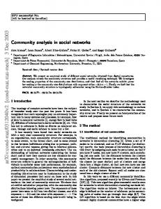
C. Correlation between Features Figure 1 shows the correlation between different features of Table I. The correlation is measured as the absolute value of Spearman’s rank correlation coefficient between different features. In order to better visualize the correlations, the rows and coloumns of the heat-map are clustered to create blocks of highly correlated features. For instance, Density, ClusteringCoefficient, AverageDegree, and AverageCloseness features are correlated as expected. Note that, their corresponding temporal features are also correlated with each other. However, as we can see in these heat-maps, most of the defined features are not

Fig. 2. Enron: The number of times a feature is selected by the 10 predictive models (left), and the correlation between each feature and response variable (right).

different features and the response variables is also depicted in Figure 2. Here, to calculate correlation between features and cohesion, and size transitions, we consider their cohesive, and expand values respectively. Furthermore, to simplify the comparison between this heat-map and the one showing the selection of the features, the rows are ordered correspondingly. Similar to the number of times that a feature is selected, the correlation between each feature and response variables differs for different response variables. Moreover, the correlation of a feature is positively correlated with the number of times it is selected.

Fig. 1. Absolute value of Spearman’s rank correlation coefficient between different features. Top: Enron, Bottom: DBLP. These correlation matrices depict that the overlap between features used in our predictive models is low.

highly correlated in neither Enron nor DBLP. This behaviour is desirable, since we define features to capture different properties of a community and its temporal changes. In other words, the low correlation/ overlap between features confirms that the features used in our predictive models are distinctive. D. Ensemble Analysis Any of the predictive models we introduced, selects a different set of features. We consider a feature is more prominent for a specific event or transition, if it is selected by the majority of the models trained for predicting that event or transition. Figure 2 shows the number of times that each feature is selected by our 10 predictive models for predicting each event. Here, to better visualize the selection of the features, only the rows of the heat-map is clustered to create blocks of similarly colored cells. The Pearson correlation between

We can infer interesting patterns form this ensemble analysis. For example ClusteringCoefficient and Cohesion are prominent positive factors on the survival of Enron communities, while StableLeaderTopics and LeftNodesRatio are important negative factors on survival. The importance of these factors on survive is intuitive, for instance, a community with high clustering coefficient has strong relationship between its members and will not dissolve easily. On the other hand, loosing members (i.e. high LeftNodesRatio) is a good sign of an unstable community which is not going to survive. In case of split, LeadersRatio and NodesNumber are positively important, i.e. a community with more leaders or a bigger size community is more probable to split. Whereas, the negative effect of VarianceCloseness and Cohesion shows that a community with high variance of closeness scores and high cohesion is immune to split. The merge of a community is positively influenced by StableTopics, talking about the same topics over the time leads the community to merge with another communities. On the other hand, Similarity has negative influence on merge, i.e. a community with almost stable members is not probable to merge with others. Similarly, the ensemble analysis for DBLP is depicted in Figure 3. Again, interesting patterns can be inferred from these two heat-maps. For instance, Density is a positive factor in size transition, whereas, NodesNumber is negatively important, i.e. a dense community attract new members and expands, while a bigger size community has less chance to attract new members. We also observe that Cohesion is a prominent negative feature on the cohesion transition of a community in

of preferential attachment phenomenon in [14], [15] or the modelling of the node arrival and edge creations in [16]. On the other end, the macroscopic perspectives study the evolution of the high level properties of networks, for instance, the study of the evolution of degree distribution, clustering coefficient, and degree correlation of online social networks in [17], or the study of shrinking diameter of social networks in [18].

Fig. 3. DBLP: The number of times a feature is selected by the 10 predictive models (left), and the correlation between each feature and response variable (right).

Fig. 4. Comparison of prominent features on the ENRON (left) and DBLP (right) dataset. Only features that are selected more than five times by at least one event or transition are included.

a later snapshot. This importance indicates that on DBLP, a less cohesive community has a better potential to form new connections and become more cohesive. Comparing the features importance between these two datasets, we see that these patterns although similar, depend on the underlying dynamic social network. This finding demonstrates the importance of the feature selection step for the prediction task. Figure 4 provides the comparison between prominent features selected for the two dataset. Here, we only include the features that are selected more than five times by at least one (event or transition) predictive models. The diagrams show that, for instance on DBLP, JoinNodesRatio is influential for all the five events and transitions. On the other hand, StableLeaderTopics is influential in only size, and cohesion prediction. V.

R ELATED W ORK

The works on evolution of dynamic networks can be classified into three categories: microscopic, macroscopic and mesoscopic approaches. The microscopic approaches focus on the evolution at the level of nodes and edges, such as the study

Different models are proposed to predict microscopic or macroscopic trends of dynamic networks. Notably, Yang et al. [19] develop a prediction model to analyze the loss of a user in an online social network, by extracting a set of attributes and using a decision tree classifier. Huang and Lee [20], propose a model to select the most influential activity features, and then incorporate these features to predict the growth or shrinkage of the network. Based on their findings, on the Facebook data, the number of active members and the number of edges is the most informative factors to predict the network evolution. Whereas, on the Citeseer data, it is observed that the number of collaborations between members is the main indicator to explain the evolving patterns of this co-authorship network. A less explored perspective is provided by the mesoscopic approaches, which predict the trend of networks based on an intermediate structure of the networks, i.e. community structure. The evolution of communities from the standpoint of growth is modeled in [21]–[23], where an individual in a community never leaves the community, i.e. a community in these studies always grows. For instance, Backstrom et al. [21] apply a decision-tree approach by incorporating a wide range of structural features to predict whether and entity will join a community. Given a community, they also predict its growth over a fixed time period. Patil et al. [24] build a classifier to predict if a community is going to grow or is likely to remain stable over a period of time. However, they only consider explicit communities, for instance, conferences are considered as communities for the DBLP dataset. Kairam et al. [25] identify two types of growth for a community. Diffusion growth is when a community attracts new members through ties to existing members; whereas, in non-diffusion growth, individuals with no prior ties become members themselves. Their analysis is then focused on the differences in the processes which govern diffusion and non-diffusion growth. Their finding shows that if a community is highly clustered, it is more likely to experience diffusion growth. However, communities that grow more from diffusion tend to reach smaller final sizes. They also generated a set of models which use a community’s structural features and past growth experience to predict its eventual size and lifespan. The works mentioned above consider explicit communities, and can only be applied in the settings where users join multiple communities and probably never quit these communities. Thus, the size of a community will monotonically increase over the time. However, in most networks, an individual may quit his/her current community and join another one, in case he/she is not satisfied with that community. Hence, the communities in these dynamic networks usually have fluctuating members and could grow and shrink over the time. In the case of implicit communities, Goldberg et al. [26], [27] develop a linear regression system to predict the lifespan of a community based on structural features extracted from the early stage of the community. They find that community’s

properties such as size, intensity and stability are the most important features to predict its lifespan. The most relevant work to ours is of Brodka et al. [28], [29], where they develop different classifiers to predict the events that may occur for a community (similarly defined as continue, merge, split, and dissolve). Their model is trained mainly based on the history of events happened to the community in preceding snapshots. Therefore, events can only be predicted for communities that their past three instances is available. While these instances also have to be in consecutive snapshots. Another drawback of their approach is that they consider events to be mutually exclusive and only predict the dominating event. In our model, however, the future of a community is predicted based on an extensive set of features on its current members, their roles and their relations, where we also leverage temporal information (up to one time-frame backward), if the previous instances of the community are available. Also using the notion of metacommunity, we are able to track multiple events and transitions that a community undergoes in non-consecutive snapshots. VI.

C ONCLUSION

We investigated the evolution of dynamic networks, at the level of their community structure. We defined and extracted an extensive set of relevant role-based, structural, contextual and temporal features, to represent the the structural and nonstructural properties of communities and the behaviour of their (influential) members. Our experimental results on realworld datasets (Enron and DBLP) shows that the defined features are mainly non-overlapping, and distinctive. Based on which, the events and transitions of communities can be accurately predicted. Our predictive process also identifies the most prominent features for each community transition and event. We confirm the relation between the behavior of individuals, specially the influential members of a community, and the future of the community they belong to, and also observe many interesting, yet expected, evolution patterns, e.g. recruiting new members by a community is a good indicator of its survival.

[10] [11]

[12]

[13]

[14] [15]

[16]

[17]

[18]

[19]

[20]

[21]

[22]

[23]

[24]

R EFERENCES [1] [2]

[3]

[4]

[5]

[6] [7]

[8] [9]

J. Leskovec, L. A. Adamic, and B. A. Huberman, “The dynamics of viral marketing,” ACM Transactions on the Web, vol. 1, p. 5, 2007. H. Akhlaghpour, M. Ghodsi, N. Haghpanah, V. S. Mirrokni, H. Mahini, and A. Nikzad, “Optimal iterative pricing over social networks,” in Internet and Network Economics, 2010, pp. 415–423. N. Agarwal, H. Liu, L. Tang, and P. S. Yu, “Identifying the influential bloggers in a community,” in International Conference on Web Search and Data Mining, 2008, pp. 207–218. M. McPherson, L. Smith-Lovin, and J. M. Cook, “Birds of a feather: Homophily in social networks,” Annual Review of Sociology, vol. 27, no. 1, pp. 415–444, 2001. A. Anagnostopoulos, R. Kumar, and M. Mahdian, “Influence and correlation in social networks,” in ACM SIGKDD International Conference on Knowledge Discovery and Data Mining, 2008, pp. 7–15. S. Goel and D. G. Goldstein, “Predicting individual behavior with social networks,” Marketing Science, vol. 33, no. 1, 2014. M. Takaffoli, F. Sangi, J. Fagnan, and O. R. Za¨ıane, “Tracking changes in dynamic information networks,” in International Conference on Computational Aspects of Social Networks, 2011. A. Abnar, “Structural social role mining,” Master’s thesis, University of Alberta, 2014. I. H. Witten, G. W. Paynter, E. Frank, C. Gutwin, and C. G. NevillManning, “KEA: Practical automatic keyphrase extraction,” in ACM Conference on Digital Libraries, 1999, pp. 254–255.

[25]

[26]

[27]

[28]

[29]

N. Landwehr, M. Hall, and E. Frank, “Logistic model trees,” Machine Learning, vol. 59, no. 1-2, pp. 161–205, 2005. M. Hall, E. Frank, G. Holmes, B. Pfahringer, P. Reutemann, and I. H. Witten, “The weka data mining software: an update,” ACM SIGKDD explorations newsletter, vol. 11, no. 1, pp. 10–18, 2009. J. Chen, O. R. Za¨ıane, and R. Goebel, “Detecting communities in large networks by iterative local expansion,” in International Conference on Computational Aspects of Social Networks, 2009, pp. 105–112. N. V. Chawla, K. W. Bowyer, L. O. Hall, and W. P. Kegelmeyer, “SMOTE: Synthetic minority over-sampling technique,” Artificial Intelligence Research, vol. 16, pp. 321–357, 2002. A.-L. Barab´asi and R. Albert, “Emergence of scaling in random networks,” Science, vol. 286, no. 5439, pp. 509–512, 1999. E. Elmacioglu and D. Lee, “Modeling idiosyncratic properties of collaboration networks revisited.” Scientometrics, vol. 80, no. 1, pp. 195–216, 2009. J. Leskovec, L. Backstrom, R. Kumar, and A. Tomkins, “Microscopic evolution of social networks,” in ACM SIGKDD International Conference on Knowledge Discovery and Data Mining, 2008, pp. 462–470. Y.-Y. Ahn, S. Han, H. Kwak, S. Moon, and H. Jeong, “Analysis of topological characteristics of huge online social networking services,” in International Conference on World Wide Web, 2007, pp. 835–844. J. Leskovec, J. Kleinberg, and C. Faloutsos, “Graphs over time: Densification laws, shrinking diameters and possible explanations,” in ACM SIGKDD International Conference on Knowledge Discovery in Data Mining, 2005, pp. 177–187. T. Yang, Y. Chi, S. Zhu, Y. Gong, and R. Jin, “A bayesian approach toward finding communities and their evolutions in dynamic social networks,” in SIAM International Conference on Data Mining, 2009. S. Huang and D. Lee, “Exploring activity features in predicting social network evolution,” in IEEE International Conference on Machine Learning and Applications, 2011, pp. 7–15. L. Backstrom, D. Huttenlocher, J. Kleinberg, and X. Lan, “Group formation in large social networks: membership, growth, and evolution,” in ACM SIGKDD international conference on Knowledge discovery and data mining, 2006, pp. 44–54. E. Zheleva, H. Sharara, and L. Getoor, “Co-evolution of social and affiliation networks,” in ACM SIGKDD international conference on Knowledge discovery and data mining, 2009, pp. 1007–1016. A. Mislove, M. Marcon, K. P. Gummadi, P. Druschel, and B. Bhattacharjee, “Measurement and analysis of online social networks,” in ACM SIGCOMM conference on Internet measurement, 2007. A. Patil, J. Liu, and J. Gao, “Predicting group stability in online social networks,” in International Conference on World Wide Web, 2013, pp. 1021–1030. S. R. Kairam, D. J. Wang, and J. Leskovec, “The life and death of online groups: Predicting group growth and longevity,” in ACM International Conference on Web Search and Data Mining, 2012, pp. 673–682. M. Goldberg, M. Magdon ismail, S. Nambirajan, and J. Thompson, “Tracking and predicting evolution of social communities,” in International Conference on Social Computing, 2011, pp. 7–15. M. K. Goldberg, M. Magdon-Ismail, and J. Thompson, “Identifying long lived social communities using structural properties,” in International Conference on Advances in Social Networks Analysis and Mining, 2012, pp. 647–653. P. Br´odka, P. Kazienko, and B. Koloszczyk, “Predicting group evolution in the social network,” in International Conference on Social Informatics, 2012, pp. 54–67. B. Gliwa, P. Br´odka, A. Zygmunt, S. Saganowski, P. Kazienko, and J. Kozlak, “Different approaches to community evolution prediction in blogosphere,” in International Conference on Advances in Social Networks Analysis and Mining, 2013, pp. 1291–1298.