Comparative performance of logistic regression

This article was downloaded by: [University of California, San Diego] On: 18 April 2013, At: 11:33 Publisher: Taylor & Francis Informa Ltd Registered in England and Wales Registered Number: 1072954 Registered office: Mortimer House, 37-41 Mortimer Street, London W1T 3JH, UK

International Journal of Geographical Information Science Publication details, including instructions for authors and subscription information: http://www.tandfonline.com/loi/tgis20

Comparative performance of logistic regression and survival analysis for detecting spatial predictors of land-use change a

b

c

a

Ninghua Wang , Daniel G. Brown , Li An , Shuang Yang & Arika Ligmann-Zielinska

d

a

Joint Ph.D. Program in Geography, San Diego State University and University of California, Santa Barbara, CA, USA b

School of Natural Resources and Environment, University of Michigan, Ann Arbor, MI, USA c

Department of Geography, San Diego State University, San Diego, CA, USA d

Department of Geography, Michigan State University, East Lansing, MI, USA Version of record first published: 18 Apr 2013.

To cite this article: Ninghua Wang , Daniel G. Brown , Li An , Shuang Yang & Arika LigmannZielinska (2013): Comparative performance of logistic regression and survival analysis for detecting spatial predictors of land-use change, International Journal of Geographical Information Science, DOI:10.1080/13658816.2013.779377 To link to this article: http://dx.doi.org/10.1080/13658816.2013.779377

PLEASE SCROLL DOWN FOR ARTICLE Full terms and conditions of use: http://www.tandfonline.com/page/terms-andconditions This article may be used for research, teaching, and private study purposes. Any substantial or systematic reproduction, redistribution, reselling, loan, sub-licensing, systematic supply, or distribution in any form to anyone is expressly forbidden. The publisher does not give any warranty express or implied or make any representation that the contents will be complete or accurate or up to date. The accuracy of any instructions, formulae, and drug doses should be independently verified with primary

Downloaded by [University of California, San Diego] at 11:33 18 April 2013

sources. The publisher shall not be liable for any loss, actions, claims, proceedings, demand, or costs or damages whatsoever or howsoever caused arising directly or indirectly in connection with or arising out of the use of this material.

International Journal of Geographical Information Science, 2013 http://dx.doi.org/10.1080/13658816.2013.779377

Comparative performance of logistic regression and survival analysis for detecting spatial predictors of land-use change Ninghua Wanga *, Daniel G. Brownb , Li Anc , Shuang Yanga and Arika Ligmann-Zielinskad


a

Joint Ph.D. Program in Geography, San Diego State University and University of California, Santa Barbara, CA, USA; b School of Natural Resources and Environment, University of Michigan, Ann Arbor, MI, USA; c Department of Geography, San Diego State University, San Diego, CA, USA; d Department of Geography, Michigan State University, East Lansing, MI, USA (Received 11 July 2012; final version received 12 February 2013) Although survival analysis is known to outperform logistic regression, theoretically and according to evidence from other disciplines, little is known about how true this is in situations where the goal is detecting spatial predictors of land change. Furthermore, with the increasing availability of longitudinal land-change data, evidence is needed on the relative performance of these two different methods in situations with differing levels of data abundance. To fill this gap, we generated a pseudo land-change data set using an agent-based model of residential development in a virtual landscape. This agent-based model simulated the decisions of homebuyers in choosing residential locations based on the values of several spatial variables. Pseudo land-change maps, generated by the agent-based model with different weights on these spatial variables, were exposed to statistical analysis under the logistic and survival approaches. We evaluated how well the two approaches could reveal the spatial variables that were used in the agent-based model and compared the performance of the two methods when land-change data were collected under different sampling frequencies. Our results suggest that survival analysis outperforms logistic regression in detecting the variables that were included in agent decisions, largely because it takes into account time-dependent variables. Also, this research suggests that various properties of land-change processes (like amount of developed area and access of agents to information) affect the relative performance of these statistical approaches aimed at uncovering land-change predictor variables. Keywords: land-change science; survival analysis; logistic regression; space-time analysis; pseudo data set; agent-based model

1.

Introduction

Most land-change studies involve two steps: detecting changes in land use or land cover and relating these changes to some set of predictive or causal factors (Lambin and Geist 2006). Detecting land changes is by no means simple, but advances in the acquisition, processing, and interpretation of remote sensing imagery over the past two decades have made this task less daunting (Green et al. 1994, Lunetta et al. 2006, Turner et al. 2007). In comparison, however, explaining the observed changes, that is, identifying spatial predictor variables and their relative contributions, still remains challenging. Too many plausible predictor

*Corresponding author. Email: [email protected] © 2013 Taylor & Francis


2

N. Wang et al.

variables exist, and their effects vary greatly over space, time, and specific context (Geist and Lambin 2002). In recent years, impressive efforts have been made to integrate remote sensing imagery and socioeconomic data (Liverman 1998). These integrated data sets hold great promise for identifying predictors of land change, provided appropriate analytical methods are applied to them. Turner et al. (1996) were among the first to suggest using logistic regression for this task. Because logistic regression is more appropriate for use with categorical outcomes, like land-cover classes, than ordinary least square regression (Lambin 1997, Overmars and Verburg 2005), it soon became widespread in land-change science (Serneels and Lambin 2001, Aspinall 2004, Geist and Lambin 2004, Huang et al. 2007, Wyman and Stein 2010). For urban applications, Wu and Yeh (1997) analyzed the impact of land reform policy on Chinese urban growth. Their logistic model gave very different estimates (sign and magnitude) on the same land-change predictor variables, suggesting the structural difference in urban development before and after the reform. Cheng and Masser (2003) continued this effort by applying logistic regression, coupled with satellite imagery of 1993 and 2000, and GIS, on Wuhan, a transportation hub in central China. Their model revealed the fading role of master planning in urban development, with the rise of decentralized decision making. In sum, results of these analyses have contributed considerably to the current knowledge and understanding of variables associated with various land-change outcomes. The growing availability of land-change data, often based on satellite imagery, over multiple time intervals and longer time extents (Mertens and Lambin 2000, Vagen 2006, Zhou et al. 2008), presents a challenge for use of logistic regression. When analyzing longitudinal land-change data, logistic regression does not effectively use prior-change temporal information. In other words, a change occurring at the beginning of the observation extent is weighed the same as one occurring toward the end of the observation extent. As a result, the significance of a variable’s contribution may be very dependent upon the length of the observation extent. To circumvent this challenge, a recent study (Huang et al. 2009) has introduced an exponential smoothing technique on three logistic models that were developed on three consecutive time periods (1984–1992, 1992–1997, and 1997–2002). The smoothing function assigned relatively higher weights on more recent observations than older ones. This multi-temporal logistic model effectively predicts land-use change in New Castle County, Delaware, yet the use of parameters in the smooth function and the relationship to the land-change time remain unclear and are subject to uncertainty. Survival analysis provides an alternative analytical framework for dealing with longitudinal data. Originating in biomedical research, this framework soon gained popularity in many other disciplines where the timing of events is of concern, for example, machine failure (Cox and Oakes 1984, Mudholkar et al. 1995, Klein and Moeschberger 1997) and divorce (Smith and Zick 1994, Yashin et al. 1995, Allison 2001, Lee and Wang 2003). This framework evaluates causative contributions to the occurrence and timing of the event of interest. Survival analysis has also found its way to land-change science (Irwin and Geoghegan 2001, An et al. 2011), where it has been demonstrated as a valuable approach to revealing the varying effects of predictor variables on land changes over time. In theory, survival analysis should outperform logistic regression, as it uses information more fully. Mathematical analysis has shown that survival analysis is superior when the duration is long and changes are frequent (Green and Symons 1983). This theoretical conclusion, though it has been verified in fields such as medical science (Green and Symons 1983), is not fully tested in application of land-change analysis. Land-change science differs from other fields in its explicit incorporation of spatial and temporal complexities in land-change processes. Both survival analysis and logistic regression have strength in


International Journal of Geographical Information Science

3

modeling individual behaviors, but as land is inherently continuous, how to define the individual land unit becomes a problem (An and Brown 2008). Two data models are most common in GIS applications: the raster and vector models. The raster model simplifies the space as a grid of cells, which provides convenience for data handling but short in realistic mapping of natural entities such as mountains and lakes. The vector model, on the other hand, represents a space consisting of recognizable objects, following their natural shapes, for example, lakeshores or coastlines. Recent application of high resolution remote sensing imagery has moved towards reconciling this choice: on the one hand, satellite imagery can be easily converted to raster data; on the other hand, pixels in high resolution image are fine enough to capture changes in parcel lots where land-change decisions are usually made. In addition to spatial complexity, many characteristics of land, for example, soil fertility and population density, may change over time, which may directly or indirectly influence the direction or rate of land change, adding another layer of temporal complexity. Data of higher temporal resolution allow the measure of these dynamic characteristics, but we also need metrics to associate them to land-change events. Survival analysis holds promise for this aspect because it can accommodate explanatory variables with varying values over time (Allison 2001), which may help to uncover some mechanisms of land change that could not be revealed by other statistical models. However, it is important to note that each statistical framework involves a different set of assumptions. Survival analysis is relatively more complex than logistic regression and has higher requirements on the time resolution of data. As such, the relative performance of each statistical framework needs to be compared under different circumstances as a way to improve their use in analyses of land-change processes. After reviewing literature on logistic regression and survival analysis with considerations on model choice, we pursued the following specific research question in this study: How much and under what circumstances does survival analysis perform better than logistic regression in detecting predictors of land change? To answer this question, we evaluated and compared the performances of statistical models estimated under these two frameworks using data on land-change outcomes whose underlying mechanisms are well known. The mechanisms were specified in an agent-based model of residential growth. We varied the magnitude of land changes, the level of determinism in the agent decisions, the temporal frequency of sampling for the land-change outcomes, and the time-varying predictor variables. Statistical model parameters retrieved by the different statistical methods were compared with the known predictor variables used in the agent-based model to test the accuracy of the different statistical methods under different modeling and sampling conditions. We limited land changes in the model to those from non-urban use to urban use, which is mostly irreversible (except over very long time period), as a case study. We acknowledge that there are other types of land changes that are reversible, for example, between pasture and forest. We concentrated our research on land-use change from non-urban to urban, however, because (1) the non-urban to urban change is common and important in nearly all countries (Angel et al. 2005) and (2) methodologically, it is fundamental, as a reversible land change can be decomposed into a chain of short irreversible changes. Nonetheless, the results of our comparison do not directly apply to reversible land changes. It is important to note that such changes are particularly complicating, and our survival analysis framework would need to be modified to address irreversible changes, which goes beyond the scope of this study. Section 2 reviews these two statistical frameworks and their variants. After important applied situations are reviewed, the research methods and experimental design are

4

N. Wang et al.


described in Sections 3 and 4. Results are presented in Section 5, and Sections 6 and 7 discuss implications and conclusions. 2. Regression analysis Regression analysis is commonly used when measuring correlations between a dependent or response variable and some number of covariates. The distinction between statistical correlation and causation has been elaborated elsewhere (Holland 1986) and must always be considered when regression is used to evaluate causal relationships. In the context of land-change science, land changes are widely understood to result from land managers’ decisions (Briassoulis 2000, Geist and Lambin 2004, Turner et al. 2007), and factors that stimulate or constrain land managers’ decisions can be considered as land-change predictors. From a pool of potential predictor variables that are informed by theories (Angelsen and Kaimowitz 1999, Irwin and Geoghegan 2001, Walker 2004) and experts’ opinions, those showing significant correlations to land-change events (P-value < 0.05) are often identified as the predictors accounting for land change. Because most predictor variables are spatial in nature, effects of spatial autocorrelation should be taken into account, otherwise P-values can be inflated and false conclusions may arise. 2.1. Logistic regression Logistic regression was originally used in modeling binary outcomes with a suite of explanatory variables, for example, a customer’s purchase decision of a product may relate to product characteristics or demographic, social, and geographic factors associated with the individual. For land-change science, researchers aim to associate binary land status, for example, changed or not, with a suite of biophysical or socioeconomic variables to explain land-change processes. Because of the categorical nature of the outcomes, logistic regression was easily adapted for studying predictor variables in land-change applications (Coomes et al. 2000, Cheng and Masser 2003, Huang et al. 2007, 2009, López and Sierra 2010, Wyman and Stein 2010). In particular, the maximum likelihood estimation allows modelers to evaluate influences from categorical covariates, for example, gender or ethnicity (Overmars and Verburg 2005), which has improved the analytical power of regression in land-change applications. The most common form of logistic regression uses the logit link function (Equation 1), where Pi is the land-change probability of location i, β 0 is the intercept, and X 1 to Xk are k covariates (i.e., predictors variables) that help explain land status (denoted as Xki for value at location i), which can be numerical or categorical. Note all variables are italic and same hereafter. Logit (Pi ) = β0 + β1 X1i + β2 X2i + . . . + βk Xki

(1)

Despite many advantages, logistic regression suffers an important difficulty for modeling processes with multiple time measures. If both land types and covariates change values over time, logistic regression has to use either the value at one time or the average over time, which results in loss of information and reduction in degrees of freedom (An and Brown 2008) An alternative form of logistic regression, the survey logistic model (‘survey’ model hereafter) uses piecewise data restructuring (Appendix A). Instead of one probability for


5


each observation or location, which might be thought of as parcels or pixels in the context of land change, each location can have multiple probabilities, determined by the number of ‘piecewise’ periods. A location–period probability Pij is defined as the probability that location i experiences land change at period j. This Pij is linked to a period-specific intercept β 0j and covariates X 1 through Xk of their values at location i and period j (denoted as Xkij in Equation 2). Please note that covariate Xkij may vary over periods. It is called a survey model because it can group observations from the same unit (e.g., location or household) into a cluster, a technique often used to deal with correlations in survey data (Singer and Willett 2003) and in a similar manner to piecewise longitudinal data. Because the survey model uses the latest values of predictor variables of every period, it can handle time-dependent covariates. Logit (Pij ) = β0j + β1 X1ij + β2 X2ij + . . . + βk Xkij

(2)

2.2. Survival analysis Survival analysis is a collection of methods explicitly dealing with the occurrence and timing of events. As a framework specialized for event data, survival analysis is well suited to handle three types of temporal complexities. First, survival analysis quantifies the potential risk of an event using a ‘hazard’ metric. This hazard metric depends on not only the number of events occurred but also their timing. For example, large numbers of events or early events correspond to higher hazard and vice versa. So events at different time points are weighed differently. Second, survival analysis not only includes samples in which events take place within the observation extent, but also samples that experience events of interest before or after the observation extent. The latter two cases are called samples censored at left and right, respectively. Sometimes survival analysis can also include interval censored data, where samples have events within an interval, but the exact times are unknown. Third, survival analysis allows for covariates with time-varying values, that is, timedependent covariates. For example, the population density of an area may increase and decrease over time. Survival analysis uses the updated population density to estimate the hazard of a location in that area. In sum, these features allow survival analysis to use more temporal information, minimizing uncertainties in the estimation process. As such, survival analysis has gained attention in land-change science (Irwin and Bockstael 2004, Iovanna and Vance 2007, An and Brown 2008, An et al. 2011). It is worth noting, however, that survival analysis is predominantly applied to study death or other irreversible processes. Although many land changes are irreversible, some are reversible, which may present limits to the applicability of survival analysis. Interpretation of survival models is similar to logistic regression, for example, the evaluation of significance of covariates, except (1) the dependent variable is hazard instead of probability and (2) intercept h0 (t)can be a function of time (Equation 3). Log hi (t) = Log h0 (t) + β1 X1i (t) + β2 X2i (t) + . . . + βk Xki (t)

(3)

where hi (t) is the hazard of location i at time t, h0 (t) is the baseline hazard shared by all locations, and Xk is the kth covariate.

6

N. Wang et al.


In survival analysis, the form of the intercept function Log h0 (t) is usually difficult to specify. There are generally two ways to solve this problem: parametrically using a piecewise exponential model (Allison 2001) and semi-parametrically using the Cox proportional hazard (PH) model (Cox 1972). The piecewise exponential model (‘piecewise’ model hereafter) breaks the entire study time extent into a certain number of periods and approximates the intercept in period j to a constant β 0j (Equation 4). When periods are sufficiently short, this approximation is quite reasonable. The Cox PH model (‘Cox’ model hereafter), in comparison, circumvents the task of specifying the intercept function by dividing hazards of early events over hazards of later events. Because all hazards share the same intercept function, it cancels out. As such, coefficients β 1 to β k are directly estimated from hazard ratios. For more details, please refer to Allison (2001). Log hi (t) = β0j + β1 X1ij + β2 X2ij + . . . + βk Xkij

(4)

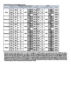
where j = 1,2,. . .J , J is the number of periods. Xkij is the value of nth predictor at location i in period j (note that Xkij may have different values over periods). hi (t) is the hazard of location i at time t. In sum, two analytical frameworks in four variants were examined (Table 1). Table 1 also lists the assumptions, data distributions, and calibration algorithms of these statistical methods. 3. Model selection As in any statistical analysis, selection of model form is critical in land-change science (Agarwal et al. 2002, Parker et al. 2003, Lambin and Geist 2006), yet systematic explorations of the behaviors and suitabilities of different model forms have not been done adequately (Turner et al. 2001). Models are instruments of inquiry for specific purposes. So the appropriateness of a model is first evaluated by whether it serves the research purpose, in our case to identify land-change predictors. After the purpose is clear, we need to Table 1.

Summary of statistical models examined in this study. Logistic

Model Response variable distribution Link function Independent variable distribution Time-varying independent variable? Intercept Assumption Calibration algorithm Diagnostic methods

Logit

Survival Survey

Cox

Piecewise

Binary or discrete

Discrete and/or continuous

Logit function Continuous and categority, okay on non-normality No Yes

Hazard function Continuous and categority, okay on non-normality

Constant Piecewise asymptote asymptote MLE MLE ROC, deviance, goodness-of-fit, generalized R2

Canceled Piecewise PH assumption constant interval P-MLE MLE Generalized R2 , schoenfeld residual, deviance, martingale residual

Yes

Yes



7

consider a number of factors, such as assumptions, temporal data completeness, and levels of complexity (Allison 2001, Harrell 2001). First, all models make assumptions to provide simplified representations of the real world. Statistical models function properly only when the assumptions are good approximations of the situations represented in the data. The Cox model, for example, assumes that covariates (i.e., predictor variables) exert constant influences on hazards over time, a.k.a. the PH assumption (Singer and Willett 2003). The piecewise model assumes constant effects within each time period. These assumptions may be violated in the case of rapid land-change processes. For example, in a competitive land market, land desirability (or hazard) would increase over time as land resource is exhausted. In that way, covariates’ effects on land desirability inflate rapidly with time, violating the PH assumption. Second, different models differ in whether they handle time discretely or continuously. However, as the discrete time intervals shrink, it is not always clear when to switch to a continuous-time model. As land-change science shifts to interest in and availability of fine temporal resolution data, we need to know when survival analysis will produce better results. Third, land changes occur within complex socio-ecological systems. Modelers have to strike a balance between taking adequate account of system complexity on one the hand and seeking an explicable, parsimonious model on the other. Agarwal et al. (2002) outlined three dimensions of complexity for socio-ecological systems: spatial, temporal, and human decision-making. Specific modeling approaches are often strong at modeling complexity in one dimension, but weak in others. So model selection depends upon the dimension(s) of complexity that modelers intend to address. 4. Methods We used a diverse set of land-change conditions to test alternative statistical models. We adopted a novel computational approach as follows (Figure 1). With a specific set of variables and parameters, we (1) simulated a land-change process, (2) sampled the data that resulted from that process spatially and temporally following specific rules, (3) exposed the sampled data to statistical models of interest, and (4) evaluated those models by comparing their coefficients to the actual parameters we programmed for a given simulation. This evaluation procedure was repeated 1000 times over different model variables and parameter values, both selected by the Monte Carlo technique. 4.1. Simulation approach To evaluate the performance of statistical models under a range of conditions, we simulated those conditions by using a Monte Carlo technique to generate results from an agent-based model of LUCC under a sample of parameter combinations. We generated data through simulation, as opposed to empirically, for three reasons. First, a simulated data set minimizes uncertainties in model assessment, which often arise when assessing statistical methods with real data because it is possible only to hypothesize about what are the underlying mechanisms by using various theories, experts’ opinions, and statistical evaluation methods. It is not possible to know for certain, or to manipulate with experimental control, the underlying mechanisms generating a real-world data set. However, by using a simulation approach, the underlying mechanisms, variables, and parameters are completely known and the ability of statistical models to recover them can be accurately assessed (Hirzel et al. 2001).


8

N. Wang et al.

Figure 1. Steps involved in evaluation of statistical results in the context of each land-change process.

Second, comparing methods using empirical case study data, as has been done in previous work (Malanson 2005, An and Brown 2008, Pontius et al. 2008), limits the applied situations under which the methods can be explored. Different land-change processes involve different predictor variables (An and Brown 2008, Rindfuss et al. 2008, An et al. 2011), changing at different speeds (Lambin and Geist 2006) and involving different levels of information access by land managers and users (Manson 2006). These factors lead to diverse land-change pathways. Constructing an empirical data set that represents a wide range of pathways is very difficult, but relatively easy for a simulation data set where alteration of the simulation program’s initial parameters produces a diverse set of pathways (Clarke et al. 2007, Rindfuss et al. 2007). As such, we can map the relative performance of each statistical technique across applied situations. Third, the simulation approach enables full control of data production and ensures data completeness (Neel et al. 2004, Epperson et al. 2010). Data completeness refers to the resolution and extent of data coverage. It is a key factor in model selection (Harrell 2001), and it is often limited spatially and temporally in real data sets. To study the sensitivity of statistical models to these kinds of limits, we test models on data sets sampled at different frequencies. There is a risk that virtual land-change processes generated by a certain simulation program may lack generality, limiting range of conditions under which conclusions about the efficacy of statistical methods may apply. In this study, we replicated all our experiments using a second simulation program (Ligmann-Zielinska and Sun 2010). This agent-based modeling (ABM) program is a simplified implementation of a residential development process, focusing on site suitability assessment and investment decisions. Because of


9


space limit, replication details and results are presented in Appendix B and in online supplementary document. 4.2. Simulation model Developed by the Spatial Land Use Change and Ecological Effects (SLUCE) project (http://www.cscs.umich.edu/sluce/ ), the SOME (SLUCE’s Original Model for Experimentation) model was selected for our study because of its parsimonious representation of land dynamics using ABM techniques (Brown et al. 2005). ABM is a category of computational models that directly simulates the behaviors of individual agents (Parker et al. 2003), where agents act autonomously in the course of simulation, following rules designed by modelers. SOME consists of three primary parts: a virtual landscape, a group of agents representing homebuyers, and their behavior rules. The land market is simplified by considering demand only, while the supply of homes always meets demand. The landscape in SOME is a lattice of cells of equal size. Each homebuyer acquires one and only one cell, which is then converted to residence, resulting in land-use change. The global land-use change pattern is a consequence of location decisions by a sequence of homebuyers. Homebuyers evaluate cells based on a utility function ux,y (t) (Equation 5), where x and y are coordinates of a given cell and select from a pool of candidate cells the one with highest utility. ux,y (t) = (AQx,y (t))αAQ × (1/SCx,y (t))αSC × (1/Wx,y )αW

(5)

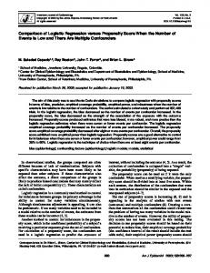
It is not possible to include all land-change driving forces in any given simulation. For simplicity, we included three potential variables in utility function, aesthetic quality (AQ), distance to service center (SC), and distance to water (W ). The influences by these variables are adjusted by α AQ , α SC , and α W , whose values we alternate between 0 and 1 for these experiments. We assumed a lake on the left border of the landscape, so W is the Euclidean distance from the border. SC is the Euclidean distance to the nearest service center. Initially, we place a service facility at the center of the landscape. As the simulation continues, a new service facility is added to the landscape for each additional set of 100 homebuyers; the location of the service facility is near the location chosen by the last homebuyer. This process continues until a certain proportion of the landscape is occupied or a specified number of time steps has passed. The AQ value is derived from a predetermined 121 by 121 random map of AQ with positive spatial autocorrelation (Figure 2). This positively autocorrelated map was generated by (1) creating 100 random points, each with a random value, (2) applying a kriging interpolation on those points to smooth the surface, and (3) dissecting a 121 by 121 grid from the virtual terrain. Developments (residents and service centers) at nearby locations, defined by a 3 × 3 window around each cell, negatively affect the AQ value of that cell by a constant fraction each time a new development is created. For more information about SOME, please refer to An et al. (2005) and Brown et al. (2005). We chose AQ, SC, and W for the following reasons. First, they represent biophysical and socioeconomic variables, two general categories most common in land-change processes. Second, they possess a wide range of time variability: W has a fixed value over time, with development, AQ, and SC decrease over time. Predictor variables from the real world would mostly fall into this range. Figure 3a, b, and c shows how land-change patterns are affected by AQ, SC, and W , respectively.


10

N. Wang et al.

Figure 2. Virtual landscape of aesthetic quality considering spatial autocorrelation.

Figure 3. Land-change patterns created when agents consider only (a) aesthetic quality (AQ), (b) distance to service center (SC) or (c) distance to water (W ) in their utility calculation.

4.3. Experimental procedures To learn the relative performance of statistical models, we tested them each for a wide range of land-change conditions. Theory and applications in other domains show that survival analysis outperforms logistic regression, so an experiment over all conditions should reproduce this finding. Further, an examination of variations between conditions would inform us of the relative performance of each method in different application situations. In particular, land-change conditions are simulated as follows. First, we ran the model with each predictor turned on (α = 1) and off (α = 0), respectively, resulting in eight conditions, for example, all on or off, one on and the other two off, or one off and the other two on. This approach is to simulate the challenge in identifying effective variables from a pool of potential ones (Hersperger and Bürgi 2009). In addition, we selected two parameters out of a dozen from SOME and swept all values over their ranges. The first parameter, called numresidents, controls the amount of land change that the model produces by determining how many residents enter. For every simulation step, the same number of residents (numresidents) enters the landscape. When



11

numresidents is high, more land is developed at every step, so there will be more changes across space and over time. The second parameter, called numtests, controls the number of candidate cells that a homebuyer evaluates when searching the landscape. High numtests implies high level of access to information about available land. Candidate cells are drawn randomly, in attempt to represent realistic conditions of personal preference, institutions, and other constraints on access to land information. High numtests reduces process randomness, resulting in more deterministic spatial patterns and temporal dynamics of land change. On the contrary, low numtests results in stochastic development patterns in space and time. We acknowledge that in real world, there may be more land-change pathways that cannot be controlled by these two parameters. However, we would like to choose them because (1) they determine the quantity and spatial distribution of land change (Figure 4) and (2) they affect the validity of some statistical assumptions (e.g., PH assumption in the Cox model) when their values go to extremes. We used the Monte Carlo technique to produce land-change conditions from a large number of possibilities (Table 2). Because numtests and numresidents are continuous measures, we grouped their values for analysis into a priori ranges, determined through a sensitivity analysis, and uniformly sampled within each range (Figure 4). We sampled 1000 specific land-change conditions, from the full set of possible parameter combinations, on our workstation (Dell Precision T5400 Intel Xeon 3.16 GHz Qual-core 16G memory). 4.4. Space–time sampling Mapped results from the above land-change simulations were sampled spatially and temporally. A combined sampling scheme of systematic and random sampling (Cheng and Masser 2003, Luo and Wei 2009) was adopted to minimize autocorrelation while maintaining the representativeness of samples. We tested the residuals of regression analysis and found that as the sample size decreased from 20% to 5%, Moran’s I decreased from 0.23 (z-score = 4.02, positive autocorrelation) to 0.027 (z-score = 1.46, no autocorrelation). Also, 5% sampling at different time points maintained a Moran’s I of less than 0.1, with z-score 0.05) when the corresponding factor is turned ‘off’ (α equals ‘0’). A model was considered fully successful if all predictor variables were correctly detected. The rates of partial and full success usually turned out to be the same in our experiments, so we report only the full success rate, except for the section on time-dependent variables and in Figure 6, where the partial success rate was used.

5. Result 5.1. Overall performance Of the 1000 Monte Carlo experiments, the piecewise model achieved the highest (full) success rate (Figure 5). The Cox model, a variant of survival analysis, received the second highest success rate. No logistic model had a success rate above 40%.

Figure 5. Overall full success rates of the different statistical models, after 1000 Monte Carlo experiments.


14

N. Wang et al.

Figure 6. The relative partial success rates for different models on the time-independent variable (W ) and the time-dependent variables (AQ and SC).

Besides the success rate, logistic regressions were diagnosed by statistical indicators, including over-dispersion, lack of fit, and Receiver Operating Characteristic (ROC) curve. No over-dispersion was found (P-value = 0.99 for deviance rejected the over-dispersion hypothesis) in the response variable, and logistic models showed good fit to data from tests on ROC (average = 0.92, SD = 0.16) and Hosmer and Lemeshow goodness-of-fit (P-value = 0.91, where goodness-of-fit is rejected when P-value < 0.05). Still, different statistical indicators could reveal different aspects of the model, and the success rate proposed by us presented some new information. This Monte Carlo result helps us understand how survival analysis performs relative to logistic regression. However, to understand the application situations over which each statistical model is effective, we need to further explore the results of 1000 experiments.

5.2. Time-dependent and -independent variables Different land-change predictors show different levels of temporal variability, that is, some predictors (e.g., distance to water) have fixed values over time, while others (e.g., distance to service center and aesthetic quality) change values with land developments. In general, it is more difficult to measure the effects of time-dependent predictors. However, it is commonplace to have time-dependent predictors in land-change process models, for example, population density. Using the partial success rates, we evaluated every statistical model for success in detecting the importance of each variable (Figure 6). All statistical models performed better in detecting the time-independent variable, W , than in detecting time-dependent variables, SC and AQ (except in the Cox model, AQ has higher success rate). The success rate for W ranges from a high value of 94%, for the piecewise model, to a low value of 82%, for the logit model. Time-dependent variables were more difficult to detect with success rate ranging from 88% to 54%. While success rates for detecting the time-independent variables and time-dependent variables were different among all statistical models, the differences were larger for the


15


logistic models. The survey model had the largest difference (41%) and the logit model the second largest (30%). In contrast, the differences for two survival models were much lower (12% for the Cox model and 9% for the piecewise model). This indicates a greater consistency in model performance for the survival models compared to the logistic models. 5.3. Development percentage and information access Monte Carlo experiments over nine different combinations of values of the two continuous parameters, numresidents and numtests in Figure 4, revealed considerable variability in full success rates (Figure 7). The piecewise model outperformed other models for almost every combination, except in combination e, where the logit model performed equally well. Also, the piecewise model did not show much variability across different parameter combinations, indicating that it is a robust model for dealing with various land-change situations. The logit model performed well when the development percentage was at medium level (e.g., combinations b, e, and h in Figure 7), but worse when the development percentage was low or high. This finding is consistent with literature (Cramer 1999, King and Zeng 2001), in which extreme binary ratios, that is, data dominated by 1’s or 0’s, deteriorates model performance. In the context of land change, situations such as rare changes or ubiquitous changes are not appropriate for the logit model. In theory, high information access would pose a challenge to the PH assumption of the Cox model, since high information access leads to more competition for the same land parcels and, therefore, scarce land resources. As such, the effects of covariates on land attractiveness would appear to increase over time, which challenges the PH assumption that covariates hold constant effects over time. This challenge, however, does not produce serious bias according to our results. The Cox model maintains high success rate (>65%) in situations with high information access, unless the development percentage is also high (success rate = 55% at combination i). 5.4. Sampling frequency Sampling frequency had an impact on the Cox, piecewise, and survey model and no impact on the logit model, which only uses data at two times (one at the beginning of the run and one at the end). Although the sampling frequency has a direct effect on the piecewise model and the survey models, by determining into how many ‘pieces’ the longitudinal data will be segmented, the effect on the Cox model is less obvious, in that it affects the calculation of hazard. Nonetheless, the general effect on the success rate is the same: because at higher

Figure 7. Full success rates of statistical models for each combination of development percentage (numresidents) and information access (numtests).


16

N. Wang et al.

Figure 8. The impacts of sampling frequency on full success rates.

frequencies, more temporal information is retained, statistical models are more likely to detect the corresponding land-change variables, whereas at lower frequencies they are less likely to detect variables (Figure 8). All models except the logit model performed better when the sampling frequency was higher, that is, more samples over time, because more information is used.

6. Discussion This study used simulation data to investigate the performance of survival analysis and logistic regression in different applied situations. This simulation approach provided us the convenience to preset predictors of land change and test if they are reflected in statistical results. Also, it could span a wide range of land-change conditions, making it possible to evaluate statistical methods in different situations and in the future to explore their application domains. In detecting spatial predictors of land change, our experiments with simulated data have shown that survival analysis consistently outperformed logistic regression. This finding conforms to theory, corroborating the usefulness of our simulation approach. Among many survival models, the piecewise model has better revealed the role of spatial predictor variables. Full use of information and less violation to model assumptions may explain why the piecewise model performed the best. Among logistic models, the logit model was better than the survey model, which may be explained by the severe imbalance between ‘0’ and ‘1’ in piecewise data (see below). More importantly, we explored the relative performance of the two methods in different application situations regarding temporal characteristics of effective predictors, the percentage of development, the level of information access, and data completeness. All these factors could impose challenges to the task of detecting predictor variables, limiting the application situations of statistical models.



17

One important temporal complexity in land-change science is the changing characteristics of some environmental factors over time or time-dependent variables. Survival models are advantageous in detecting time-dependent variables, that is, where the value of a predictor variable changes over time (Allison 2001, An and Brown 2008). Survival models associate changes in land hazards to changing values of time-dependent variables, so estimate accurately the effects of these variables. Logistic models overlook time variability of variables, so when time-dependent variables are present, they are prone to erroneous estimates. Logistic models did not perform well when the amount of development was very low (75%). In fact, logistic models require balanced binary values, that is, similar numbers of ‘0’ and ‘1’ (Cramer 1999, King and Zeng 2001, Heinze and Schemper 2002, Fletcher et al. 2005). This finding has important implications for landchange studies. Many land-change cases are either very slow, for example, established urban areas in developed countries, or very fast, for example, deforestation in frontiers. These situations may lead to unbalanced land outcomes that pose challenges to logistic models. Cheng and Masser (2003) and Huang et al. (2009) indirectly solved this unbalanced data issue by applying two different sampling schemes to converted and unconverted land separately. Nonetheless, when the total amount of converted or unconverted land is small, sampling a fraction of land, for example, 5%, will result in a very small sample size. As such, it might be difficult to fulfill sample size requirement. Land development leads to land resource depletion. However, according to the mechanisms in the SOME model, when information access is high or, in other words, when the candidate pool is large, lands with high covariate values are always included in the candidate pool and quickly depleted. As a result, lands with lower covariate values become competitive for later time since high value lands are gone. In other words, the same covariate has increased impact on the hazard of being developed (Figure 9). This outcome essentially violates the PH assumption that covariates exert constant effect to the hazard over time. While in theory this might be the case, in experiments we found that for Cox model, moderate violation of this assumption did not have detectable effects on our results.

Figure 9. Land resource depletion over time causes inflated effect of covariates on hazard, illustrated by W as the major factor. Note that low W is preferred (closer to water) but over time lands far from water are developed.


18

N. Wang et al.

The performance of survival models hinges on sampling frequency. High frequency improves performance because more dynamic information is captured. Performance of the logit model, in contrast, is independent of sampling frequency, because it includes only two states of land (e.g., the beginning and final states) in its analysis. In general, survival models are recommended unless temporal information is limited; when this limit exists, the logit model should be considered with concerns about its other conditions (e.g., balance between ‘0’s and ‘1’s). For the purposes of evaluating alternative statistical models, the simulation approach seems to be very useful. It complements conventional applications of statistical models to empirical data in at least two respects. First, by simulating land-change processes, the variables and parameters that are used to generate a given pattern are known completely, and statistical modeling results can be compared to those known characteristics. Second, a rich and diverse set of land-change processes can be generated, as opposed to one or a few that might be contained in an empirical setting, providing us insights into the usefulness of alternative statistical models under a diverse range of conditions. Although the neartransparent quality of simulated data has been often used in other domains to quantify modeling results (Foss et al. 2003, Burton et al. 2006), it is less common in geography (Hirzel et al. 2001) and has never been applied to assess the ability of statistical models to detect predictor variables in land-change applications. There is a risk that virtual processes do not reflect the wide range of possible underlying processes very well, introducing limits to the generality of the results. In this study, we reduced this risk by several means: (1) to validate our findings, we used another simulation program, which was independently developed based on different assumptions and conceptualizations, and the match of results corroborates our findings (Appendix B); (2) the Monte Carlo technique we employed randomly sampled the parameter space of our simulation program, allowing comprehensive assessment of various situations under which our land-change model might function; and (3) we tested all possible combinations of predictor variables, for example, the eight cases in our study. This mimicked the situation in which we are unaware of the true predictor values and have to make decisions from a pool of potential predictors. This research investigated the relative performance of survival analysis and logistic regression using data from non-urban to urban land, a common land-change type that has been well studied (Lambin 1997, Cheng and Masser 2003, Huang et al. 2009). It may also represent a wide range of land-change types that are irreversible or unidirectional. However, some conversions are reversible, for example, two-way changes between tilled and untilled agricultural land or between pasture and forest. These reversible land changes, or multi-event (on the same land unit) processes, certainly complicate the application of survival analysis, and these complications may present situations in which survival analysis is less suitable for application. It is possible to segment a reversible land-change into a series of irreversible changes, and variants of survival analysis have been reported to be able to handle multi-event processes (Allison 2001, Andersen and Keiding 2002). Future studies will need to test survival analysis methods on reversible land changes. If the simulation approach is used, the selected simulation model needs to reflect this type of multi-event process accordingly. Several new directions will be explored in the future. First, this simulation study should be linked to empirical studies. We are in the process of collecting satellite imagery and socioeconomic data in a time series and experiment with how the increase in temporal resolution of data affects statistical results. Second, we could more thoroughly appraise statistical models using other non P-value indicators, such as coefficients of covariates. Third,


19

survival models should be integrated with land-change analysis more tightly in terms of method and conceptualization. Our experimentation reveals the practical aspects of survival analysis in probing simulated dynamic land-change systems. Since survival analysis outperforms other analytical techniques when temporal variability is present (e.g., dynamic factors), it can be utilized in studies where disturbances, abrupt events, and policy interventions are introduced into the system. Not only do such disruptions change the dynamics of land patterns, but they may also affect the predictors themselves.


7. Conclusion This study confirms the theoretical speculation that survival models generally perform better than logistic models using simulation-based land-change data. This may arise from survival models’ more effective use of temporal information. We present our findings in the hope that more research would be devoted to this type of models in land-change analysis. Furthermore, this study provides insights into the relative performance of survival models and logistic models, an important step towards better defining application domains of these methods. It appears that survival models perform better in detecting time-dependent variables and are robust to handle very fast/slow land-change processes and varying levels of information access. Logistic models are not recommended when very fast or slow land-change processes give rise to highly unbalanced land outcomes (i.e., nearly all developed or undeveloped) or when information access is extremely high or low. The only time logistic regression might be recommended is when samples in time are very sparse. The simulation approach is useful when assessing the inferential power of statistical models in land-change studies. One advantage that cannot be otherwise obtained is its endowment of a land-change researcher’s better control of experiment processes (thus less ‘noise’ or unknown processes), allowing for potentially more accurate assessment of different statistical models when applied in different land-change situations. Acknowledgments This research was funded by National Science Foundation: the Biocomplexity in the Environment Program (BCS-0119804) and SLUCE II project (GEO-0814542), the Partnership for International Research and Education (PIRE; OISE-0729709) Program, and the Dynamics of Coupled Natural and Human (CNH) Systems (DEB-1212183) Program. It was also supported by 2) SDSU UGP Project under the title ‘Sampling at What Scales? A Computational Simulation Approach’. The authors thank three anonymous reviewers for their valuable comments and suggestions.

References Agarwal, C., et al., 2002. A review and assessment of land-use change models: dynamics of space, time, and human choice. USA: Forest Service. Northeastern Research Station. Allison, P., 2001. Survival analysis using the SAS system: a practical guide. Cary, NC: SAS Publishing. An, L. and Brown, D., 2008. Survival analysis in land change science: integrating with giscience to address temporal complexities. Annals of the Association of American Geographers, 98, 323–344. An, L., et al., 2005. What statistical models help to detect land-change mechanisms? GeoComputation 2005, Ann Arbor, Michigan. An, L., et al., 2011. Variations in development of exurban residential landscapes: timing, location, and driving forces. Journal of Land Use Science, 6, 13–32. Andersen, P.K. and Keiding, N., 2002. Multi-state models for event history analysis. Statistical Methods in Medical Research, 11, 91–115.


20

N. Wang et al.

Angel, S., et al., 2005. The dynamics of global urban expansion. Transport and Urban Development Department, The World Bank, Washington D.C., 1, 1–11. Angelsen, A. and Kaimowitz, D., 1999. Rethinking the causes of deforestation: lessons from economic models. The World Bank Research Observer, 14, 73–98. Aspinall, R., 2004. Modelling land use change with generalized linear models–a multi-model analysis of change between 1860 and 2000 in Gallatin Valley, Montana. Journal of Environmental Management, 72, 91–103. Briassoulis, H., 2000. Analysis of land use change: theoretical and modeling approaches. Available from: http://www.rri.wvu.edu/WebBook/Briassoulis/contents.htm [Accessed 21 January 2012]. Brown, D., et al., 2005. Path dependence and the validation of agent-based spatial models of land use. International Journal of Geographical Information Science, 19, 153–174. Burton, A., et al., 2006. The design of simulation studies in medical statistics. Statistics in Medicine, 25, 4279–4292. Cheng, J. and Masser, I., 2003. Urban growth pattern modeling: a case study of Wuhan city, PR China. Landscape and Urban Planning, 62, 199–217. Clarke, K.C., et al., 2007. A decade of SLEUTHing: lessons learned from applications of a cellular automaton land use change model. In: P. Fisher, ed. Classics in IJGIS: Twenty Years of the International Journal of Geographical Information Science and Systems, Boca Raton, FL: Taylor & Francis, 413–427. Coomes, O., Grimard, F., and Burt, G., 2000. Tropical forests and shifting cultivation: secondary forest fallow dynamics among traditional farmers of the Peruvian Amazon. Ecological Economics, 32, 109–124. Cox, D.R., 1972. Regression models and life-tables. Journal of the Royal Statistical Society. Series B, Methodological, 34, 187–220. Cox, D.R. and Oakes, D., 1984. Analysis of survival data. Boca Raton, FL: Chapman & Hall/CRC. Cramer, J.S., 1999. Predictive performance of the binary logit model in unbalanced samples. Journal of the Royal Statistical Society: Series D (The Statistician), 48, 85–94. Epperson, B., et al., 2010. Utility of computer simulations in landscape genetics. Molecular Ecology, 19, 3549–3564. Fletcher, D., MacKenzie, D., and Villouta, E., 2005. Modelling skewed data with many zeros: a simple approach combining ordinary and logistic regression. Environmental and Ecological Statistics, 12, 45–54. Foss, T., et al., 2003. A simulation study of the model evaluation criterion MMRE. Software Engineering, IEEE Transactions on, 29, 985–995. Geist, H. and Lambin, E., 2002. Proximate causes and underlying driving forces of tropical deforestation. Bioscience, 52, 143–150. Geist, H. and Lambin, E., 2004. Dynamic causal patterns of desertification. Bioscience, 54, 817–829. Green, K., Kempka, D., and Lackey, L., 1994. Using remote sensing to detect and monitor land-cover and land-use change. Photogrammetric Engineering and Remote Sensing, 60, 331–337. Green, M.S. and Symons, M.J., 1983. A comparison of the logistic risk function and the proportional hazards model in prospective epidemiologic studies. Journal of Chronic Diseases, 36, 715–723. Harrell, F., 2001. Regression modeling strategies: with applications to linear models, logistic regression, and survival analysis. New York: Springer Verlag. Heinze, G. and Schemper, M., 2002. A solution to the problem of separation in logistic regression. Statistics in Medicine, 21, 2409–2419. Hersperger, A.M. and Bürgi, M., 2009. Going beyond landscape change description: quantifying the importance of driving forces of landscape change in a Central Europe case study. Land Use Policy, 26, 640–648. Hirzel, A., Helfer, V., and Metral, F., 2001. Assessing habitat-suitability models with a virtual species. Ecological Modelling, 145, 111–121. Holland, P.W., 1986. Statistics and causal inference. Journal of the American Statistical Association, 81, 945–960. Huang, Q., Cai, Y., and Peng, J., 2007. Modeling the spatial pattern of farmland using GIS and multiple logistic regression: a case study of Maotiao River Basin, Guizhou Province, China. Environmental Modeling and Assessment, 12, 55–61. Huang, B., Zhang, L., and Wu, B., 2009. Spatiotemporal analysis of rural–urban land conversion. International Journal of Geographical Information Science, 23, 379–398. Iovanna, R. and Vance, C., 2007. Modeling of continuous-time land cover change using satellite imagery: an application from North Carolina. Journal of Land Use Science, 2, 147–166.



21

Irwin, E. and Bockstael, N., 2004. Land use externalities, open space preservation, and urban sprawl. Regional Science and Urban Economics, 34, 705–725. Irwin, E.G. and Geoghegan, J., 2001. Theory, data, methods: developing spatially explicit economic models of land use change. Agriculture, Ecosystems & Environment, 85, 7–24. King, G. and Zeng, L., 2001. Logistic regression in rare events data. Political Analysis, 9, 137. Klein, J. and Moeschberger, M., 1997. Survival analysis: techniques for censored and truncated data. New York: Springer-Verlag. Lambin, E., 1997. Modelling and monitoring land-cover change processes in tropical regions. Progress in Physical Geography, 21, 375. Lambin, E.F. and Geist, H., 2006. Land-use and land-cover change: local processes and global impacts. New York: Springer Verlag. Lee, E.T. and Wang, J.W., 2003. Statistical methods for survival data analysis. Hoboken, NJ: Wiley & Sons, Inc. Ligmann-Zielinska, A., 2009. The impact of risk-taking attitudes on a land use pattern: an agent-based model of residential development. Journal of Land Use Science, 4, 215–232. Ligmann-Zielinska, A. and Sun, L., 2010. Applying time dependent variance-based global sensitivity analysis to represent the dynamics of an agent-based model of land use change. International Journal of Geographical Information Science, 24, 1829–1850. Liverman, D.M., 1998. People and pixels: linking remote sensing and social science. Washington, D.C.: National Academies Press. López, S. and Sierra, R., 2010. Agricultural change in the Pastaza River Basin: a spatially explicit model of native Amazonian cultivation. Applied Geography, 30, 355–369. Lunetta, R.S., et al., 2006. Land-cover change detection using multi-temporal MODIS NDVI data. Remote Sensing of Environment, 105, 142–154. Luo, J. and Wei, Y.H., 2009. Modeling spatial variations of urban growth patterns in Chinese cities: the case of Nanjing. Landscape and Urban Planning, 91 (2), 51–64. Malanson, J., 2005. Comparison of the structure and accuracy of two land change models. International Journal of Geographical Information Science, 19, 745–748. Manson, S.M., 2006. Bounded rationality in agent-based models: experiments with evolutionary programs. International Journal of Geographical Information Science, 20, 991–1012. Mertens, B. and Lambin, E., 2000. Land-cover-change trajectories in southern Cameroon. Annals of the Association of American Geographers, 90, 467–494. Mudholkar, G.S., Srivastava, D.K., and Freimer, M., 1995. The exponentiated Weibull family: a reanalysis of the bus-motor-failure data. Technometrics, 37, 436–445. Neel, M.C., McGarigal, K., and Cushman, S.A., 2004. Behavior of class-level landscape metrics across gradients of class aggregation and area. Landscape Ecology, 19, 435–455. Overmars, K. and Verburg, P., 2005. Analysis of land use drivers at the watershed and household level: linking two paradigms at the Philippine forest fringe. International Journal of Geographical Information Science, 19, 125–152. Parker, D., et al., 2003. Multi-agent systems for the simulation of land-use and land-cover change: a review. Annals of the Association of American Geographers, 93, 314–337. Pontius, R., et al., 2008. Comparing the input, output, and validation maps for several models of land change. The Annals of Regional Science, 42, 11–37. Rindfuss, R.R., et al., 2007. Frontier land use change: synthesis, challenges, and next steps. Annals of the Association of American Geographers, 97, 739–754. Rindfuss, R.R., et al., 2008. Land use change: complexity and comparisons. Journal of Land Use Science, 3, 1–10. Serneels, S. and Lambin, E.F., 2001. Proximate causes of land-use change in Narok District, Kenya: a spatial statistical model. Agriculture, Ecosystems & Environment, 85, 65–81. Shuster, J.J., 1992. Practical handbook of sample size guidelines for clinical trials. Boca Raton, FL: CRC Publishing. Singer, J.D. and Willett, J.B., 2003. Applied longitudinal data analysis: modeling change and event occurrence. USA: Oxford University Press. Smith, K.R. and Zick, C.D., 1994. Linked lives, dependent demise? Survival analysis of husbands and wives. Demography, 31, 81–93. Turner, M.G., Gardner, R.H., and O’neill, R.V., 2001. Landscape ecology in theory and practice: pattern and process. New York: Springer Verlag.


22

N. Wang et al.

Turner, B.L., Lambin, E.F., and Reenberg, A., 2007. The emergence of land change science for global environmental change and sustainability. Proceedings of the National Academy of Sciences, 104, 20666. Turner, M.G., Wear, D.N., and Flamm, R.O., 1996. Land ownership and land-cover change in the Southern Appalachian Highlands and the Olympic Peninsula. Ecological applications, 6, 1150–1172. Vagen, T.G., 2006. Remote sensing of complex land use change trajectories–a case study from the highlands of Madagascar. Agriculture, Ecosystems & Environment, 115, 219–228. Walker, R., 2004. Theorizing land-cover and land-use change: the case of tropical deforestation. International Regional Science Review, 27, 247. Wu, F. and Yeh, A.G.O., 1997. Changing spatial distribution and determinants of land development in Chinese cities in the transition from a centrally planned economy to a socialist market economy: a case study of Guangzhou. Urban Studies, 34, 1851–1879. Wyman, M. and Stein, T., 2010. Modeling social and land-use/land-cover change data to assess drivers of smallholder deforestation in Belize. Applied Geography, 30, 329–342. Yashin, A.I., Vaupel, J.W., and Iachine, I.A., 1995. Correlated individual frailty: an advantageous approach to survival analysis of bivariate data. Mathematical Population Studies, 5, 145–159. Zhou, Q., Li, B., and Kurban, A., 2008. Trajectory analysis of land cover change in arid environment of China. International Journal of Remote Sensing, 29, 1093–1107.

Appendix A. Piecewise data restructuring A common practice in longitudinal data analysis is to conduct piecewise data restructuring for some type of analysis (Shuster 1992). Because of various reasons such as data availability or the researcher’s intentional choice, the entire time extent may be divided into several periods, which are usually, but not necessarily, of equal length (Allison 2001, 109). For all the periods during which the individual (person, location, or whatever unit under consideration) is at risk, we record the information related to all the dependent and independent variables, forming data of so-called individual-periods. In such individual-periods, a specific independent variable may take changing or constant values depending on whether it is a time-dependent variable, and the dependent variable may be the survival time within that specific period and the associated censoring status, or a binary development status, depending on the type of model that is to be constructed. A common concern may be the lack of independence among the individual-periods from the same individual, which has been shown not to be a problem in the survival analysis literature (Allison 1995, 108, 223–225).

B. IDEAL model and results The agent-based model called IDEAL is similar in design to SOME in terms of landscape (lattice of cells) and agents. What sets them apart, however, are the rules agents use to make land purchase decisions. In IDEAL, at each simulation step, all agents investigate available land parcels and make up a preference list, which depends upon land characteristics, their own demands, and their attitude toward risk represented using gains and losses (Ligmann-Zielinska 2009). The agents evaluate available land parcels using the ideal point (IP) decision rule. Agents compare available lands against the best and worst cases in the landscape and, according to their own attitude toward risk, reassess land drivers and assign weights to the parcels. When a parcel is favored by more than one agent, this conflict is resolved by assigning that parcel to the agent who has highest preference order, and a tie is resolved randomly. These mechanisms altogether, as it turns out, render a land-change process drastically different from that of SOME. We ran IDEAL over 1000 runs including three variables: beauty, land value, and water access. Because developments affect beauty and land value (Ligmann-Zielinska and Sun 2010), their values vary over time. The water access variable, on the other hand, remains constant throughout the time. The level of information access and the development percentage are controlled by parameters sample_size and demand, which are uniformly sampled in nine ranges (Figure 4). Experiments on IDEAL revealed similar patterns to those observed for SOME across logistic models and survival models. The piecewise model had the highest success rate and the Cox model, the survey model, and the logit model had the second, third, and lowest rates, respectively. For the


23

logistic models, it was more difficult to detect the time-dependent variable (beauty and land value) than the time-independent one (water access). Low information access and high development percentage posed challenges on the logit model, but had little influence on survival models. As we sampled less frequently, the success rate decreased for all models except the logit model, whose rate remained the same. Refer to online supplementary document for figures.

C. SAS code to implement statistical models


The logit model is implemented by the LOGISTIC procedure. Because the simulation starts from an empty landscape, so only the final land status is enough to describe land development. The descending option helps to model type ‘1’ event (land development is denoted as finalLandType = ‘1’). proc logistic descending data= myData; model finalLandType= beauty&final distsc&final distw&final/ rsquare; run; The survey model is implemented by the SURVEYLOGISTIC procedure. ‘CLUSTER’ option is enabled to specify correlations among location-periods from the same location. In addition, the input data (myPiecewisedData) uses piecewise data restructuring (Appendix A). proc surveylogistic data= myPiecewisedData; cluster fid; model LandType= beauty distsc distw/rsquare link=glogit; run; The Cox model is realized by the PHREG procedure. This procedure first calculates the hazard from the event time and associated censoring information, then regresses the hazard against a suite of explanatory variables. PHREG procedure has several options to deal with tied event time, among which we use the exact option. proc phreg data= myData; model survival_time∗ develop(0)=beauty distscdistw/ties=exact; run; The piecewise model is realized by the LIFEREG procedure (note this model can also be implemented by LOGISTIC procedure when data time resolution is coarse (Allison 2001)). LIFEREG is able to specify the time function of hazard; here we employ the exponential function. Also, LIFEREG has not only the option for right censoring (the only option for PHREG), but also the options for left and interval censoring. To specify a unique intercept in each period, the class option is in use. In addition, the input data (myPiecewisedData) for the piecewise model needs piecewise data restructuring (Appendix A). proc lifereg data=myPiecewisedData; class step; model (lower, upper)=beauty distscdistw step/dist=exponential; run;