Comparing LTL Semantics for Runtime Verification - Christian Schallhart

Comparing LTL Semantics for Runtime Verification Andreas Bauer1 , Martin Leucker2 , and Christian Schallhart2 1

2

National ICT Australia (NICTA) Institut f¨ ur Informatik, Technische Universit¨ at M¨ unchen

Abstract. When monitoring a system wrt. a property defined in a temporal logic such as LTL, a major concern is to settle with an adequate interpretation of observable system events; that is, models of temporal logic formulae are usually infinite words of events, whereas at runtime only finite but incrementally expanding prefixes are available. In this work, we review LTL-derived logics for finite traces from a runtimeverification perspective. In doing so, we establish four maxims to be satisfied by any LTL-derived logic aimed at runtime-verification. As no preexisting logic readily satisfies all of them, we introduce a new four-valued logic RV-LTL in accordance to these maxims. The semantics of RV-LTL indicates whether a finite word describes a system behaviour which either (1) satisfies the monitored property, (2) violates the property, (3) will presumably violate the property, or (4) will presumably conform to the property in the future, once the system has stabilised. Notably, (1) and (2) correspond to the classical semantics of LTL, whereas (3) and (4) are chosen whenever an observed system behaviour has not yet lead to a violation or acceptance of the monitored property. Moreover, we present a monitor construction for RV-LTL properties in terms of Moore machines signalising the semantics of the so far obtained execution trace wrt. the monitored property.

1

Introduction

Runtime verification of a given correctness property ϕ formulated in linear temporal logic LTL [Pnu77] requires at its core the evaluation of the semantics of ϕ wrt. to a finite observed system behaviour. But the evaluation of LTL properties on finite traces proved to be an obstacle, as LTL is usually evaluated over infinite traces and since the standard semantics of LTL on finite traces [Kam68] is unsatisfactory for the purpose at hand. While the syntax and semantics of LTL on infinite traces is well accepted in the literature, there is no consensus on defining LTL over finite traces. Besides the definition in [Kam68], a number of two-valued semantics for LTL on finite traces have been proposed [GH01a,HR01b,HR02,HR01a,SB05,dR05], see Eisner et al. for a comprehensive survey on this topic [EFH+ 03]. Alternatively, it has been proposed to restrict the syntax of LTL for runtime verification, such that formulae which may contain certain future obligations cannot be specified at all [GH01b]. In monitoring a property, there arise at least three different situations: In the first case, the property is satisfied after a finite number of steps, independently of the future continuation; second, the property is shown to evaluate to false for every possible continuation, and third, the finite, already observed prefix still allows different continuations leading to either satisfaction or falsification. A prefix leading to the first (second) case is called a good (bad) prefix [KV01]. Thus, every two-valued logic must evaluate to true or false prematurely since it cannot reflect the third and inconclusive case properly. To overcome these obstacles, we propose in [ABLS05,BLS06] the three-valued logic LTL3 over finite traces. There, a property evaluates to true (false), wrt. a finite word, 1

whenever the observed word is a good (bad) prefix. In all other cases, the word is evaluated to an inconclusive verdict. This scheme matches well with the notion of safety (e. g., Gp—always p) and co-safety (e. g., F p—finally p) properties, since these are either finitely refutable or satisfiable. The union of safety and co-safety properties forms a strict subset of the monitorable properties, as defined and shown in [BLS07b]: A property is monitorable for some prefix, as long as there is some continuation leading to a good or bad prefix, i.e., as long as it is possible to arrive at a definite true or false verdict. However, there remain many properties which are non-monitorable: Consider for example the request/acknowledge property G(r → F a) which states that every request is finally acknowledged. No finite word is a good or bad prefix for G(r → F a) and therefore, this property is always evaluated to an inconclusive verdict. But since such properties arise often in practice, such a solution is quite ugly—raising the question of whether it is possible to refine the inconclusive verdict into a more telling verdict. For the request/acknowledge property, for example, we aim to have a semantics such that – a finite string ending in a (i.e., all requests have been acknowledged) yields a truth value which indicates that ϕ is probably satisfied, whereas – a finite string ending in r (i.e., there is a request not acknowledged yet) should evaluate to a truth value which expresses that ϕ is likely to remain unsatisfied. In this work, we examine how to determine a more detailed evaluation of such an inconclusive verdict. To this end, we recall in Section 3 three preexisting logics which are based upon LTL and which feature a semantics on finite words, namely FLTL [MP95], LTL∓ [EFH+ 03], as well as LTL3 [BLS06]. Since we are comparing these logics, we present them in a unified syntactical framework, outlined together with standard LTL in Section 2. Next we discuss in Section 4 the usefulness of these logics for the purpose of runtime verification. To this end, we define four maxims that we consider relevant for a linear temporal logic when using it for runtime verification. Since none of the preexisting logics satisfies all of the four maxims, we introduce in Section 5 a four-valued semantics for LTL which refines the inconclusive verdict into a presumably true and presumably false truth value. We call the resulting logic Runtime Verification Linear Temporal Logic (RV-LTL). We show that RV-LTL’s semantics indeed adheres to our four maxims and that it matches our intuition for request/response properties. RV-LTL seems to correspond to the semantics realised by the Temporal Rover [Dru00] and has, to the best of our knowledge, not been formally captured elsewhere. Finally, we define in Section 6 a translation to generate a monitor procedure in terms of a Moore machine of minimal size for each given property ϕ. Such a monitor implements the RV-LTL semantics and computes a new verdict with each upcoming state on the incrementally expanding system trace. This paper extends [BLS07a] by giving a formal treatment of the four maxims and a comprehensive comparison of LTL derived logics on finite traces, from a runtime verification perspective.

2 2.1

Preliminaries Truth domains

We consider in this paper the traditional two-valued semantics with truth values true, denoted with ⊤, and false, denoted with ⊥, next to truth values that give more information to which degree a formula is considered satisfied or not. Since truth values should be 2

comparable and combinable in terms of Boolean operations expressed by the connectives of the underlying logic, we interpret these truth values as elements of some lattice. A lattice is a partially ordered set (L, ⊑) where for each x, y ∈ L, there exists (i) a unique greatest lower bound (glb), which is called the meet of x and y, and is denoted with x ⊓ y, and (ii) a unique least upper bound (lub), which is called the join of x and y, and is denoted with x ⊔ y. A lattice is called finite iff L is finite. Every finite lattice has a well-defined unique least element, called bottom, denoted with ⊥, and analogously a greatest element, called top, denoted with ⊤. A lattice is distributive, iff x ⊓ (y ⊔ z) = (x ⊓ y) ⊔ (x ⊓ z), and, dually, x ⊔ (y ⊓ z) = (x ⊔ y) ⊓ (x ⊔ z). In a de Morgan lattice, every element x has a unique dual element x, such that x = x and x ⊑ y implies y ⊑ x. A distributive lattice is called Boolean iff x ⊔ x = ⊤ and x ⊓ x = ⊥. As the common denominator of the semantics for the subsequently defined logics is a finite de Morgan lattice, we take this to our understanding of a truth domain: Definition 1 (Truth domain). We call L a truth domain, if it is a finite de Morgan lattice. The two valued truth domain B2 = {⊥, ⊤} is a Boolean lattice with ⊥ ⊑ ⊤ and ⊓ and ⊔ defined in the expected manner. 2.2

LTL on infinite traces

As a starting point for all subsequently defined logics, we first recall linear temporal logic (LTL) interpreted over infinite traces, as introduced by Pnueli [Pnu77] in the setting of specification and verification. In case of LTL over infinite traces, one is used to have a syntax ranging over a small set of temporal and Boolean operators and to add additional operators by means of abbreviations. For example, the conjunction is often expressed indirectly using negation and disjunction—at least in the two valued truth domain. However, as several of the equivalences known from LTL over infinite traces do not hold in all the logics over finite traces considered in the paper, we start with a comprehensive—and with respect to standard LTL—redundant set of Boolean and temporal operators. We only deviate from this approach for finally (F ) and globally (G) operators, as well as for implication (→). For the remainder of this paper, let AP be a finite and non-empty set of atomic propositions and Σ = 2AP a finite alphabet . We write ai for any single element of Σ, i.e., ai is a possibly empty subset of propositions taken from AP. Finite traces (which we call interchangeably words) over Σ are elements of Σ ∗ , usually denoted with u, u′ , u1 , u2 , . . . The empty trace is denoted with ǫ. Infinite traces are elements of Σ ω , usually denoted with w, w′ , w1 , w2 , . . . For some infinite trace w = a0 a1 . . . , we denote with wi the suffix ai ai+1 . . . In case of a finite trace u = a0 a1 . . . an−1 , ui denotes the suffix ai ai+1 . . . an−1 for 0 ≤ i < n and the empty string ǫ for n ≤ i. The set of LTL formulae is defined using true, the atomic propositions p ∈ AP, disjunction, next X , and until U , as positive operators, together with negation ¬. For comparison with logics over finite traces, we moreover add dual operators, namely false, ¯ , and release R, respectively: ¬p, weak next X Definition 2 (Syntax of LTL formulae). Let p be an atomic proposition from a finite set of atomic propositions AP. The set of LTL formulae, denoted with LTL, is inductively defined by the following grammar: ϕ ::= true | p | ϕ ∨ ϕ | ϕ U ϕ | X ϕ ¯ϕ ϕ ::= false | ¬p | ϕ ∧ ϕ | ϕ R ϕ | X ϕ ::= ¬ϕ 3

Boolean constants

Boolean combinations

[w |= true]ω = ⊤ [w |= false]ω = ⊥

atomic propositions ( [w |= p]ω

=

[w |= ¬p]ω =

(

[w |= ¬ϕ]ω = [w |= ϕ]ω [w |= ϕ ∨ ψ]ω = [w |= ϕ]ω ⊔ [w |= ψ]ω [w |= ϕ ∧ ψ]ω = [w |= ϕ]ω ⊓ [w |= ψ]ω (weak) next

⊤ ⊥

if p ∈ a0 if p ∈ / a0

⊤ ⊥

if p ∈ / a0 if p ∈ a0

[w |= X ϕ]ω = [w1 |= ϕ]ω ¯ ϕ]ω = [w1 |= ϕ]ω [w |= X

until/release

[w |= ϕ U ψ]ω =

[w |= ϕ R ψ]ω =

8 > : ⊥ 8 ⊤ > > > < > > > :

⊥

there is a k ≥ 0 : [wk |= ψ]ω = ⊤ and for all l with 0 ≤ l < k : [wl |= ϕ] = ⊤ else for all k ≥ 0 : [wk |= ψ]ω = ⊤ or there is a k ≥ 0 : [wk |= ϕ]ω = ⊤ and for all l with 0 ≤ l ≤ k : [wl |= ψ] = ⊤ else

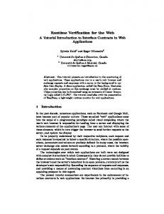
Fig. 1. Semantics of LTL formulae over an infinite traces w = a0 a1 . . . ∈ Σ ω

Moreover, we define by means of abbreviation the finally F and globally G operators as F ϕ := true U ϕ

and

Gϕ := ¬F ¬ϕ

as well as implication ϕ → ψ as a shorthand for ¬ϕ ∨ ψ. LTL formulae over infinite traces are interpreted as usual over the two valued truth domain B2 . Definition 3 (Semantics of LTL). The semantics of LTL formulae over infinite traces w = a0 a1 . . . ∈ Σ ω is given by the function [ |= ]ω : Σ ω × LTL → B2 , which is defined inductively as shown in in Figure 1. ¯ in Inspecting the semantics, we observe that there is no difference of X and X ¯ LTL over infinite traces. However, X acts differently when finite words are considered. Moreover, the semantics for a negated atomic proposition ¬p is actually given twice: once explicitly and once inductively via negation. Fortunately, both definitions coincide, ensuring that the semantics of LTL is well-defined. We call w ∈ Σ ω a model of ϕ iff [w |= ϕ] = ⊤. For every LTL formula ϕ, its set of models, denoted with L(ϕ), is a regular set of infinite traces which is accepted by a corresponding B¨ uchi automaton [VW86,Var96]. In the next section, we introduce several versions of linear temporal logics for finite traces and compare these logics by means of certain properties, such as the induced equivalences on formulae. To this end, we consider linear temporal logics L with a syntax 4

Tertium-non-datur laws ϕ ∨ ¬ϕ ≡ true ϕ ∧ ¬ϕ ≡ false

distributive laws ϕ ∨ (ψ ∧ η) ≡ (ϕ ∨ ψ) ∧ (ϕ ∨ η) ϕ ∧ (ψ ∨ η) ≡ (ϕ ∧ ψ) ∨ (ϕ ∧ η)

de Morgan-X law

de Morgan laws ¬(ϕ ∨ ψ) ≡ ¬ϕ ∧ ¬ψ ¬(ϕ ∧ ψ) ≡ ¬ϕ ∨ ¬ψ ¬¬ϕ ≡ ϕ

de Morgan-U/R laws

¯ ¬ϕ ¬X ϕ ≡ω X

¬(ϕ U ψ) ≡ ¬ϕ R ¬ψ ¬(ϕ R ψ) ≡ ¬ϕ U ¬ψ

unwinding laws ϕ U ψ ≡ ψ ∨ (ϕ ∧ X (ϕ U ψ)) ¯ (ϕ R ψ)) ϕ R ψ ≡ ψ ∧ (ϕ ∨ X

Fig. 2. Fundamental Equivalence Laws

as in Definition 2, together with a semantic function [ |= ]L : Σ ω/∗ × LTL → BL that yields an element of the truth domain BL , given an infinite or finite trace and an LTL formula. Then, for two formulae ϕ, ψ ∈ LTL, we say that ϕ is equivalent to ψ, denoted with ϕ ≡L ψ, iff for all w ∈ Σ ω/∗ , we have [w |= ϕ]L = [w |= ψ]L In particular, for LTL, we denote this equivalence by ≡ω . We say that logic L satisfies the Boolean laws if for all traces w and all formulae ϕ [w |= ϕ ∨ ¬ϕ]L = ⊤ and [w |= ϕ ∧ ¬ϕ]L = ⊥ Remark 1. LTL satisfies the Boolean laws. We say that the logic L satisfies a certain equivalence law, if its equivalences given in Figure 2 hold. We denote the equivalence laws shown there as the fundamental equivalence laws. Remark 2. LTL satisfies the fundamental equivalences laws (shown in Figure 2). While all logics studied in the next sections satisfy these equivalences, LTL is also satisfying the following variants of the de Morgan-X and respectively unwinding laws: ¬X ϕ ≡ω X ¬ϕ ϕ R ψ ≡ω ψ ∧ (ϕ ∨ X (ϕ R ψ)) Moreover, LTL satisfies true ≡ω X true These three equivalences do not hold in each of the logics discussed subsequently— resulting in a partly counterintuitive behaviour of the corresponding logic. To compare equivalences in different logics, we introduce the LTL compliance which states that every equivalence of LTL must hold in the respective logic as well: 5

Definition 4 (LTL compliance). We call a linear temporal logic L LTL compliant iff ϕ ≡ω ψ implies ϕ ≡L ψ. For its importance in various applications, we introduce the negation normal form which requires negations only to occur directly in front of atomic propositions. Definition 5 (Negation Normal Form). A formula is said to be in negation normal form, if ¬ only occurs directly in front of atomic propositions, i.e., if the formula is obtained using only the first two rules of Definition 2. Whenever the de Morgan, de Morgan-X, and de Morgan-U/R laws hold, a formula can be translated into negation normal form, and therefore, LTL has a negation normal form: Remark 3. Every LTL formula can be transformed into an equivalent formula in negation normal form.

3

LTL on Finite Traces—Existing Concepts

Let us now turn our attention to linear temporal logics over finite traces. We start by recalling a finite version of LTL on finite traces as described by Manna and Pnueli [MP95], here called. We then present Eisner’s et al.’s weak and strong versions of LTL on finite traces, denoted with LTL− and LTL+ respectively, before examining LTL3 [BLS06]. All variants, as we show, provide complementary properties for runtime verification but neither of them satisfies all our maxims put forward in Section 4. 3.1

FLTL

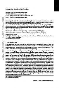
When interpreting LTL formulae over finite traces, the question arises, how to understand X ϕ when a word consists of a single letter, since then, no next position exists on which one is supposed to consider ϕ. The classical way to deal with this situation, as apparent for example in Kamp’s work [Kam68] is to understand X as a strong next operator, which is false if no further position exists. Manna and Pnueli suggest in [MP95] ¯ , which to enrich the standard framework by adding a dual operator, the weak next X allows to smoothly translate formulae into negation normal form. In other words, the strong X operator is used to express with X ϕ that a next state must exist and that this ¯ operator in X ¯ ϕ says that next state has to satisfy property ϕ. In contrast, the weak X if there is a next state, then this next state has to satisfy the property ϕ. We call the resulting logic FLTL defined over the set of LTL formulae (Definition 2) FLTL. The semantics function [u |= ϕ]F of FLTL is constructed like the one for standard LTL but with two modifications: If a strong next-state operator in some subformula X ϕ is referring to a state beyond the known finite prefix u, then this subformula X ϕ ¯ ϕ, based on the weak nextis evaluated to ⊥, regardless of ϕ. Likewise, a subformula X state operator, always evaluates to ⊤ if it refers to a state beyond u. This approach is extended to the definition of the until and release operators. For example, to satisfy ϕU ψ with a finite word u, there must exist a position satisfying ψ within u. This concept is explicated in the following definition: Definition 6 (Semantics of FLTL [MP95]). Let u = a0 . . . an−1 ∈ Σ ∗ denote a finite trace of length n, with u 6= ǫ. The truth value of an FLTL formula ϕ wrt. u, denoted with [u |= ϕ]F , is an element of B2 and is inductively defined as follows: Boolean constants, Boolean combinations, and atomic propositions are defined as for LTL (see Figure 1, taking u instead of w). Until/release and (weak) next are defined as shown in Figure 3. 6

(weak) next [u |= X ϕ]F =

(

[u1 |= ϕ]F ⊥

if u1 6= ǫ otherwise

¯ ϕ]F = [u |= X

(

[u1 |= ϕ]F ⊤

if u1 6= ǫ otherwise

until/release

[u |= ϕ U ψ]F =

[u |= ϕ R ψ]F =

8 > : ⊥ 8 ⊤ > > > < > > > : ⊥

there is a k ∈ {0, . . . n − 1} : [uk |= ψ]F = ⊤ and for all l with 0 ≤ l < k : [ul |= ϕ] = ⊤ else for all k ∈ {0, . . . n − 1} : [uk |= ψ]F = ⊤ or there is a ∈ {0, . . . n − 1} : [uk |= ϕ]F = ⊤ and for all l with 0 ≤ l ≤ k : [ul |= ψ] = ⊤ else

Fig. 3. Semantics of FLTL formulae over a trace u = a0 . . . an−1 ∈ Σ ∗

Let us first record that the semantics of FLTL is not given for the empty word. As we will see in the discussion of LTL∓ , coming up with a semantics wrt. the empty word leads to certain particularities that are hence avoided in FLTL. Since X true ≡ω true, yet the semantics of FLTL implies that a single letter does satisfy true but does not satisfy X true, we also find that FLTL is not LTL compliant. Remark 4. The semantics of FLTL formulae is not defined for the empty word. Remark 5. FLTL is not LTL compliant. It is easy to see that FLTL adheres to the Boolean laws and satisfies all fundamental equivalence laws: For example, [u |= ϕ ∨ ¬ϕ]F = [u |= ϕ]F ⊔ [u |= ϕ]F = ⊤. Likewise ¯ ¬ϕ]F follows from LTL whenever |u| > 1 and from inspecting the [u |= ¬X ϕ]F = [u |= X semantics in Figure 3 when |u| = 1. Remark 6. FLTL satisfies the Boolean laws. Remark 7. FLTL satisfies all fundamental equivalences laws (see Figure 2). In contrast to LTL, FLTL does not satisfy the following variants of the de Morgan-X ¯ used in FLTL: and respectively unwinding laws, due to the different meaning of X and X ¬X ϕ 6≡F X ¬ϕ ϕ R ψ 6≡F ψ ∧ (ϕ ∨ X (ϕ R ψ)) But since de Morgan laws are satisfied by FLTL, a negation normal form still exists for all properties. Remark 8. Every FLTL formula can be transformed into an equivalent formula in negation normal form. 7

3.2

LTL+ and LTL− —Eisner et al.

In [EFH+ 03], Eisner et al. propose two entwined versions of LTL on finite traces, reflecting a weak and a strong view. We call the resulting logics LTL− and LTL+ , respectively. If we speak of both logics at the same time, we also write LTL∓ . Recall that FLTL is not defined for the empty trace. Provided that the semantics for formulae wrt. the empty word is well-defined, one no longer needs to consider the semantics of next and until operators differently than in LTL, as done in FLTL: Having a semantics for the empty word, the evaluation of X ϕ for a word of length 1 can use the semantic value of ϕ wrt. the empty word. Likewise, for ϕ U ψ and a word u, one no longer has to require that i < |u| when considering whether ui satisfies ψ—in case i ≥ |u|, one considers ψ wrt. the empty word. LTL∓ provides a semantics for the empty word, by actually taking two approaches: In the weak view (LTL− ), every formula is satisfied by the empty word. Dually, in the strong view (LTL+ ), the empty word does not satisfy any formula. This approach leads to certain particularities: For example, in the weak view, the empty word satisfies false, while in the strong view, it does not satisfy true. Moreover, the strong and weak view have be entwined to establish a sound meaning in the context of negation: [ǫ |= ¬ϕ]+ should be ⊥ (taking the strong view) while at the same time [ǫ |= ϕ]+ = ⊥ should hold, implying that ⊥ = ⊤. LTL∓ overcomes this difficulty, by toggling between the weak and strong view whenever negation occurs, i.e., [u |= ¬ϕ]+ = [u |= ϕ]− = ⊤ (also for u = ǫ). Let us now introduce LTL∓ formally. As syntax, we consider again formulae of LTL. Though [EFH+ 03] does not provide true and false and no dual operators, these can be added with the appropriate semantics easily. Definition 7 (Semantics of LTL∓ [EFH+ 03]). Let u = a0 . . . an−1 ∈ Σ ∗ denote a finite trace of length n. The truth value of an LTL∓ formula ϕ wrt. u, denoted with [u |= ϕ]∓ , is an element of B2 and is inductively defined as follows: Boolean constants, Boolean combinations, and atomic propositions are defined as shown in Figure 4, while the semantics for the remaining formulae is as in LTL (see Figure 1, taking u instead of w). To compare LTL∓ with FLTL, and later with LTL3 , we check which of the discussed properties are satisfied by LTL3 as well: Remark 9. The semantics of LTL∓ formulae is defined for the empty trace. We can easily check that LTL∓ indeed matches our intuition: [u |= ϕ]− = ⊤, if u = ǫ [u |= ϕ]+ = ⊥, if u = ǫ We write ϕ ≡∓ ψ to denote that ϕ is both weak as well as strong equivalent to ψ, i.e., that ϕ ≡+ ψ and ϕ ≡− ψ hold. In the weak view, false holds for the empty trace, and, in the strong view, true does not hold for the empty trace. Interestingly, however, we have ϕ ∨ ¬ϕ ≡∓ true ϕ ∧ ¬ϕ ≡∓ false In consequence, for ϕ being p, we see that the Boolean laws are not satisfied by LTL∓ , as the semantics of true is not ⊤ for the empty word: Remark 10. LTL∓ does not satisfy the Boolean laws. Moreover, this implies that true is not equivalent in general to X true: While a single letter does satisfy true in the strong view, it does not satisfy X true. This implies: 8

Boolean constants

Boolean combinations

[u |= true]− = ⊤ ( ⊤ [u |= false]− = ⊥

[u |= true]+ =

(

⊤ ⊥

if u = ǫ else

[u |= ϕ]+ [u |= ϕ]− [u |= ϕ]∓ ⊔ [u |= ψ]∓ [u |= ϕ]∓ ⊓ [u |= ψ]∓

[u |= ¬ϕ]− [u |= ¬ϕ]+ [u |= ϕ ∨ ψ]∓ [u |= ϕ ∧ ψ]∓

= = = =

⊤ ⊥

if u 6= ǫ and p ∈ a0 else

⊤ ⊥

if u 6= ǫ and p ∈ / a0 else

if u 6= ǫ else

[u |= false]+ = ⊥ atomic propositions

=

(

⊤ ⊥

if u = ǫ or p ∈ a0 else

[u |= p]+

=

(

[u |= ¬p]− =

(

⊤ ⊥

if u = ǫ or p ∈ / a0 else

[u |= ¬p]+ =

(

[u |= p]−

Fig. 4. Semantics of LTL∓ formulae over a trace u = a0 . . . an−1 ∈ Σ ∗

Remark 11. LTL∓ is not LTL compliant. It is easy to see that LTL∓ satisfies all fundamental equivalence laws: Remark 12. LTL∓ satisfies all fundamental equivalences laws (see Figure 2). As de Morgan laws are satisfied by LTL∓ , the existence of the negation normal form follows: Remark 13. Every LTL∓ formula can be transformed into an equivalent formula in negation normal form. 3.3

LTL3

In[ABLS05,BLS06], we proposed LTL3 as an LTL logic with a semantics for finite traces, which follows the idea that a finite trace is a prefix of a so-far unknown infinite trace. More specifically, LTL3 uses the standard syntax of LTL as defined in Definition (2) but employs a semantics function [u |= ϕ]3 which evaluates each formula ϕ and each finite trace u of length n to one of the truth values in B3 = {⊤, ⊥, ?}. B3 = {⊤, ⊥, ?} is defined as a de Morgan lattice with ⊥ ⊏ ? ⊏ ⊤, and with ⊥ and ⊤ being complementary to each other while ? being complementary to itself. The idea of the semantics for LTL3 is as follows: If every infinite trace with prefix u evaluates to the same truth value ⊤ or ⊥, then [u |= ϕ]3 also evaluates to this truth value. Otherwise [u |= ϕ]3 evaluates to ?, i. e., we have [u |= ϕ]3 =? if different continuations of u yield different truth values. This leads to the following definition: Definition 8 (Semantics of LTL3 ). Let u = a0 . . . an−1 ∈ Σ ∗ denote a finite trace of length n. The truth value of a LTL3 formula ϕ wrt. u, denoted with [u |= ϕ]3 , is an 9

element of B3 and defined as follows:  ω   ⊤ if ∀w ∈ Σ : [uw |= ϕ]ω = ⊤ [u |= ϕ]3 = ⊥ if ∀w ∈ Σ ω : [uw |= ϕ]ω = ⊥   ? otherwise.

As opposed to the logics introduced so far, LTL3 ’s semantics is not defined in an inductive manner, i. e. the semantics of a formula is not given by the meaning of its subformulae—for good reasons: Consider a proposition p with respect to the empty word ǫ. In LTL3 , we have [ǫ |= p]3 =? = [ǫ |= ¬p]3 . The join of these values is thus ?. But in contrast, [ǫ |= p ∨ ¬p]3 = ⊤ holds, since p ∨ ¬p is a tautology3 . In other words, we have: Remark 14. The semantics of LTL3 cannot be defined inductively on the structure of the formula. Let us first recall that LTL3 is a also defined for the empty word: Remark 15. The semantics of LTL3 formulae is defined for the empty word. As LTL3 ’s semantics is derived from LTL’s semantics, we get that it is LTL compliant, as opposed to FLTL and LTL∓ . Remark 16. LTL3 is LTL compliant. As moreover true is mapped to ⊤, we get

Remark 17. LTL3 satisfies the Boolean laws. Finally, LTL3 satisfies all fundamental equivalence laws and henceforth, a negation normal form exists for all properties. Remark 18. LTL3 satisfies all fundamental equivalence laws (see Figure 2). Remark 19. Every LTL3 formula can be transformed into an equivalent formula in negation normal form.

4

Maxims for Runtime Verification of LTL Derivates

Since our original motivation is to validate common LTL-specified properties by means of runtime verification, we want to compare the applicability of logics in this context. To do so, we need to determine a frame of reference for those logics to be considered. Hence, we assume that each logic in concern is able to express syntactically all LTL-properties, and moreover, we assume that the semantics evaluation function [u |= ϕ] of the logic in concern maps each finite and non-empty word u = a0 a1 . . . an−1 ∈ Σ ∗ together with a formula ϕ to a value from a truth domain (Definition 1), such that the following rules hold for each non-empty finite word u 4 [u |= true] = [u |= p] = [u |= ϕ1 ∨ ϕ2 ] = [u |= X ϕ] = [u |= ϕ U ψ] = 3 4

⊤ ⊤ ⇐⇒ p ∈ a0 [u |= ϕ1 ] ⊔ [u |= ϕ2 ] ⊤ ⇐= |u| > 1 and [u1 |= ϕ] = ⊤ [u |= ψ] ⊔ ([u |= ϕ] ⊓ [u |= X U ψ])

Note, we call a formula ϕ a tautology, if [w |= ϕ] = ⊤ for every w. The restriction to non-empty finite words is necessary since the semantics of FLTL is not defined on empty words and because [ǫ |= true]+ 6= ⊤ in LTL+ .

10

This minimal set of requirements on [u |= ϕ] is established as the set of rules commonly shared by the logics discussed in the previous section, i.e., FLTL [MP95], LTL∓ [EFH+ 03], as well as LTL3 [BLS06]. The above rules deviate from standard LTL in the following two respects: (a) If |u| > 1 and [u1 |= ϕ] = ⊤ holds, then we require [u |= X ϕ] = ⊤ to hold—however, in contrast to LTL, we do not require the converse. (b) Negation is not guaranteed to yield a complementary truth value, i.e., we do not require [u |= ϕ] = [u |= ¬ϕ]. Starting from these core rules, we introduce four maxims which we consider essential for each semantics definition for LTL on finite traces aimed at runtime verification. The first two of them, Maxims (1) and (2), mimic and reintroduce the LTL evaluation rules which we dropped in (a) and (b)—as far as possible since we consider a semantics for LTL (on finite traces) without these rules counterintuitive: (1) Existential next requires the inclusion of a strong next operator, and (2) Complementation by negation requires that a negated formula evaluates to the complemented and different truth value. Since it is impossible to turn condition in (a) into an “if and only if”, we formulate Maxim (1) to require the next operator to behave as in LTL in as many cases as possible: Since we consider finite traces, we have to handle the semantics of X when it refers to a state beyond the currently available finite trace. To reconstitute (b), Maxim (2) reintroduces and generalises the corresponding rule of the standard semantics on infinite traces to multi-valued Boolean domains by applying the complement operator of the underlying Boolean domain. The remaining two Maxims (3) and (4) relate the semantics on finite traces with the standard LTL semantics by considering all possible continuations of the evaluated finite traces: (3) Impartiality requires that a finite trace is not evaluated to ⊤ (⊥) if there still exists an infinite continuation leading to another verdict, and (4) Anticipation requires that once every infinite continuation of a finite trace leads to the same verdict, then the finite trace evaluates to this very same verdict. By means of these four maxims, we evaluate the logics discussed in the preceding sections, i.e., FLTL [MP95] the logics LTL∓ [EFH+ 03], and LTL3 [BLS06]. As all these logics fail to satisfy all four maxims simultaneously, we introduce in Section 5 a fourvalued logic resolving the requirements imposed by the four maxims. 4.1

Approximating LTL-Semantics

We start with the first two maxims which reestablish the semantics of the next-state operator and the meaning of negation. Afterwards, we discuss the combination of these two maxims, since their combination raises some further issues. Existential Next. As discussed in [MP95], the difficulty for an LTL semantics on finite traces lies in the next-state operator X . Given a string u = a0 consisting of a single symbol, the question is which semantics to choose for X ϕ as the formula refers to an unavailable state: [u |= X ϕ] =? for |u| = 1 (1) 11

We follow the approach of [MP95] in understanding the next-state operator as an operator firstly assuring that there exists a next state which secondly satisfies ϕ. We only allow one exception to this rule: If ϕ is a tautology, then [u |= X ϕ] is also allowed to evaluate to ⊤. Without this exception, any logic satisfying our demands, would have to satisfy [u |= X true] 6= ⊤ for every word u consisting of a single symbol, which we consider counter intuitive in the setting of runtime verification. This consideration leads to the first of our four maxims: Maxim 1 (Existential Next) A logic adheres to the existential next maxim, if for every property ϕ and every finite word u ∈ Σ ∗ with [u |= X ϕ] = ⊤, one of the following two conditions holds: Either ϕ is an LTL-tautology or there exists a next state, i.e., |u| > 1, such that this next state satisfies ϕ, i.e., we require [u |= X ϕ] = ⊤ =⇒ |u| > 1 and [u1 |= ϕ] = ⊤ or |u| = 1 and ∀w ∈ Σ ω [w |= ϕ]ω = ⊤ Now, considering FLTL, we find that its semantics [u |= X ϕ]F is even more restrictive: [u |= X ϕ]F = ⊤ implies that a next state u1 exists and this next state u1 satisfies ϕ, i.e., [u |= X ϕ]F = ⊤ =⇒ |u| > 1 and [u1 |= ϕ]F = ⊤ holds. Next, the strong view of [EFH+ 03] defines a strong next operator—in precisely the same way as FLTL. On the other hand, in the weak variant LTL− of [EFH+ 03], the next operator behaves dually, i.e., [u |= X ϕ]− = ⊤ iff either u = ǫ or [u1 |= ϕ]− = ⊤, i.e., [u |= X ϕ]− = ⊤ =⇒ |u| = 0 or [u1 |= ϕ]− = ⊤ Hence, LTL+ does satisfy Maxim (1) but LTL− does not satisfy Maxim (1). Finally, the semantics of LTL3 is matching Maxim (1) since whenever a formula X ϕ evaluates to ⊤ in LTL3 , it must evaluate to ⊤ in LTL for every possible infinite continuation. Thus, we have [u |= X ϕ]3 = ⊤ iff for all w ∈ Σ ∞ [uw |= X ϕ]ω = ⊤, which is equivalent to, for all w ∈ Σ ∞ [u1 w |= X ϕ]ω = ⊤. If |u| = 1, this means that all traces satisfy ϕ, while for |u| > 1, we get [u |= X ϕ]3 = [u1 |= ϕ]3 . Thus, [u |= X ϕ] = ⊤ =⇒ |u| > 1 and [u1 |= ϕ] = ⊤ or |u| = 1 and ∀w ∈ Σ ω [w |= ϕ]ω = ⊤ Complementation by Negation. Our second maxim states that a negated formula indeed yields the complemented truth value of the original formula which must differ from the original one. We consider any other choice to be grossly counterintuitive since many fundamental relationships rely on complementary truth values for formulae and their negations. Furthermore, the requirement that the complemented truth value is different from the original one ensures that the logic does not blur the semantical evaluation into a single and non-discriminative truth value. Maxim 2 (Complementation by Negation) A logic adheres to the complementation by negation maxim, if a property ϕ and its complement ¬ϕ yield complementary and different truth values for all finite words u ∈ Σ ∗ , i.e., for each property ϕ and each finite word u, [u |= ϕ] = [u |= ¬ϕ] and [u |= ϕ] 6= [u |= ¬ϕ] must hold. 12

Recalling the logics from Section 3, we find that FLTL adheres in its definition to the requirements of Maxim (2), since we have [u |= ¬ϕ]F = [u |= ϕ]F and since FLTL is defined over a two-valued truth domain where complementary values always differ. In case of LTL+ , Maxim (2) does not hold, as can be seen in the following example with |u| = 1, [u |= ¬X p]+ = [u |= X p]− = ⊤ = ⊥ = [u |= X p]+ which holds dually for LTL− , as well. LTL3 is also not satisfying Maxim (2) since it collapses the truth values for the unforeseen future into its inconclusive truth value. It holds that [u |= ϕ]3 = ? = [u |= ¬ϕ]3 for all ϕ and u with [u |= ϕ]3 =? since whenever [u |= ϕ]3 =? holds, there must exist two infinite continuations w 6= w′ ∈ Σ ω such that [uw |= ϕ]ω = ⊤ and [uw′ |= ϕ]ω = ⊥ hold, leading to [uw |= ¬ϕ]ω = ⊥ and [uw′ |= ϕ]ω = ⊤ such that [u |= ¬ϕ]3 =? holds as well. But still, for [u |= ϕ] = ⊤ with all infinite continuations w ∈ Σ ω yielding [uw |= ϕ]ω = ⊤, we find [uw |= ¬ϕ]ω = ⊥ and hence [u |= ¬ϕ] = ⊥, such that we have [u |= ϕ]3 = [u |= ¬ϕ]3

(2)

Combining Maxims (1) and (2). Remember that we introduced Maxims (1) and (2) in order to reestablish the original LTL semantics on infinite words as much as possible. To enable an engineer to deal with LTL-specified properties intuitively, some well-known and important equivalences should hold in logics aimed at runtime verification, too. Not surprisingly, the combination of Maxim (1), demanding an existential next, and Maxim (2), requiring negation to correspond to complementation, leads to difficulties in ¬X ϕ 6≡ X ¬ϕ To see this, assume that ϕ is a formula which is neither unsatisfiable nor a tautology with respect to LTL. Then by Maxim (1), we have [u |= X ϕ] 6= ⊤ for every |u| = 1 and hence by Maxim (2) [u |= ¬X ϕ] 6= ⊥ must hold. At the same time, Maxim (1) requires [u |= X ¬ϕ] 6= ⊤ and hence we are left with the following options: (a) To use a two-valued semantics and accept ¬X ϕ 6≡ X ¬ϕ to hold, breaking with the intuitive understanding of LTL-properties. (b) To stick to the equivalence ¬X ϕ ≡ X ¬ϕ, but to use a multi-valued semantics with [u |= ¬X ϕ] = [u |= X ¬ϕ] 6∈ {⊤, ⊥} (for |u| = 1)—hereby violating Maxim (2). (c) To distinguish between a strong (denoted with X ) and a weak version (denoted with ¯ ) of the next-state operator with X ¯ ϕ] = ⊤ [u |= X and leading to

⇐⇒

|u| = 1 or [u1 |= ϕ] = ⊤

¯ ¬ϕ ¬X ϕ ≡ X

which remedies the original equivalence to a certain extent, while adhearing to Maxims (1) and (2). We call the strong next-state operator X also existential next-state ¯ operator, as it requires a next-state to exist, and the weak next-state operator X universal next-state operator. 13

Summerizing the discussion above, we remark that any logic adhearing to both Maxims (1) and (2) cannot be LTL compliant. In other words, depeding on the application, one has to choose between the Maxims (1) and (2) on the one hand side and LTL compliance on the other side. The introduction of a strong and a weak version of the next-state operator additionally allows to cope with the intuitive meaning of LTL’s finally and globally operators: Intuitively, the finally operator F is of existential nature [HR02], as some property should eventually be shown, while the globally operator G is of universal character as something should hold in every position of a word. Accordingly, F ϕ should evaluate to false if ϕ does not hold in the current state and nothing is known about the future, while Gϕ should become true, if ϕ holds in the current state and nothing is known about the successor states. Note that in LTL, we have F ϕ ≡ ϕ ∨ X F ϕ as well as Gϕ ≡ ϕ ∧ X Gϕ. Consequently, X F ϕ should be false, if no subsequent state exists, while X Gϕ should be true in the same situation. This contradiction can be resolved with the addition of the universal ¯ . Following option (c), we can rewrite the above LTL equivalences next-state operator X ¯ Gϕ. as F ϕ ≡ ϕ ∨ X F ϕ and as Gϕ ≡ ϕ ∧ X 4.2

Dealing with the Future

The so far developed view is meaningful in a setting which is only concerned with completed or terminated paths. In runtime verification, however, we are given a finite prefix of a continuously expanding trace. Therefore, it is clear that there will be a next state—this continuation is just not known yet. To reflect this situation, we postulate two further maxims for logics suitable for runtime verification. Impartiality. The first maxim says that the semantics never evaluates to true or false prematurely. In the impartiality maxim, we require a semantics never evaluates a property ϕ and a finite word u ∈ Σ ∗ to ⊤ (⊥), as long as there exists a continuation w ∈ Σ ω such that [uw |= ϕ]ω 6= ⊤ ([uw |= ϕ]ω 6= ⊥) holds. Maxim 3 (Impartiality) A logic adheres the impartiality maxim, if for each property ϕ and each finite word u ∈ Σ ∗ , [u |= ϕ] = ⊤ [u |= ϕ] = ⊥

=⇒ =⇒

∀w ∈ Σ ω ∀w ∈ Σ ω

[uw |= ϕ]ω = ⊤ [uw |= ϕ]ω = ⊥

is satisfied. Note that no two-valued logic can possibly satisfy Maxim (3) since each such logic must evaluate every property ϕ with uncertain outcome to either ⊤ or ⊥. For example, in every logic satisfying Maxim (3) we must have [u |= X p] ∈ / {⊤, ⊥} for |u| = 1. Turning again to the logics from Section 3, we find that FLTL and LTL∓ are all two-valued logics, and henceforth, they do not satisfy Maxim (3). The definition of the semantics of LTL3 on the other hand directly matches the requirements of Maxim (3), as it has been defined with this maxim in mind. Anticipation. When considering X true on a string u = a0 of length 1, there is no reason to evaluate X true to any truth value other than ⊤ since every possible continuation will satisfy X true. We therefore postulate that the semantics should be as anticipatory as possible. We say that a logic satisfies the anticipation maxim, if its semantics always evaluates a property ϕ and a finite word u ∈ Σ ∗ to ⊤ (⊥), once there exists no continuation w ∈ Σ ω such that [uw |= ϕ]ω 6= ⊤ ([uw |= ϕ]ω 6= ⊥) holds. 14

Maxim 4 (Anticipation) A logic adheres the anticipation maxim, if for each property ϕ and each finite word u ∈ Σ ∗ , the following holds: [u |= ϕ] = ⊤ [u |= ϕ] = ⊥

⇐= ⇐=

∀w ∈ Σ ω ∀w ∈ Σ ω

[uw |= ϕ]ω = ⊤ [uw |= ϕ]ω = ⊥

Maxim (4) is not satisfied by FLTL, since [u |= X true]F = ⊥ holds for |u| = 1. Similarly LTL∓ does not satisfy Maxim (4), as demonstrated by the two dual examples [u |= X true]+ = ⊥ and [u |= X false]− = ⊤, again for |u| = 1. Finally, since Maxim (4) (as well as Maxim (3)) was instrumental in the definition of LTL3 , its semantics directly reflects and hence satisfies Maxim (4).

5

RV-LTL

In the previous section, we established four maxims to be satisfied by an LTL-derived logic which is aimed at runtime verification applications. Moreover, we analysed the logics introduced in Section 3 in terms of these maxims and found that none of these logics adheres to all four maxims. To overcome this situation, we develop in this section a new logic, called Runtime Verification-LTL (RV-LTL). As in case of all other logics discussed in this paper, we use the set of LTL formulae (Definition 2) to define the syntax of RV-LTL. Since all logics in this paper are formulated atop this very same set of formulae, it is possible to combine the semantical concepts of these logics as well. Observing that LTL3 satisfies Maxims (1), (3), and (4), whereas FLTL satisfies Maxim (2), we design the semantics of RV-LTL as a combination of the semantics of LTL3 and FLTL. LTL3 matches Maxim (1) since it only evaluates a formula and a finite prefix to ⊤ if this formula will be satisfied by any possible continuation of the prefix, and that LTL3 satisfies Maxim (3) and (4) by construction—since LTL3 has been defined with these two maxims in mind. On the other hand, LTL3 does not satisfy Maxim (2), since it blurs every uncertain situation into a single inconclusive verdict: A finite word u ∈ Σ ∗ and a formula ϕ is evaluated to [u |= ϕ]3 =? whenever [uw |= ϕ]ω 6= [uw′ |= ϕ]ω holds for two infinite continuations w 6= w′ ∈ Σ ω . Since this case is arising frequently in practically important properties, the choice made in the definition of LTL3 is unsatisfactory. Consider for example the standard request/acknowledge property ϕ ≡ G(r → F a) which states that all requests must be acknowledged eventually: For every finite prefix u, we have that [urω |= ϕ]ω = ⊥ and [uaω |= ϕ]ω = ⊤ where rω and aω are infinite continuations repeating r and a ad infinitum. Therefore [u |= ϕ]3 = [u |= ¬ϕ]3 =? holds for all finite words u. Looking for a more expressive and discriminative semantics, we followed the intuition that for the property ϕ ≡ G(r → F a), we would like to have a semantics such that – a finite string ending in a (i.e., all requests have been acknowledged) yields a truth value which indicates that ϕ is probably satisfied, whereas – a finite string ending in r (i.e., there is a request not acknowledged yet) should evaluate to a truth value which expresses that ϕ is likely to remain unsatisfied. The reason for these choices are as follows: Given a finite string ending in a, all past requests have been served and therefore it remains to check that all future occurrences 15

will be served as well. Since no request is pending and the universal globally operator is dominating, we would expect the trace to be interpreted as a “presumably true” one. In case of a string ending in r, we know that there must exist a future occurrence of a in order to satisfy ϕ. Since we have a request pending and the existential eventually operator is dominating, we would expect the trace to be interpreted as a “presumably false” one. This intuition is readily expressed by the semantics of FLTL which is based upon a strong and a weak next operator. As will be discussed subsequently in this section, the existential nature of the strong next operator X translates into an existential semantics ¯ for the eventually operator F while the universal character of the weak next operator X leads to a universal semantics for the globally operator G. The problem with FLTL is that it does not distinguish between prefixes which lead to presumably true or false continuations and prefixes which lead to certainly true of false continuations, i.e., FLTL does not satisfy Maxim (3) and (4). Henceforth, we define RV-LTL as a logic which combines the semantics of LTL3 and FLTL. 5.1

Semantics of RV-LTL

To express the truth values true, false, presumably true, and presumably false, we use a four valued semantics for RV-LTL with B4 = {⊥, ⊥p , ⊤p , ⊤} as the set of truth values. Ordering ⊥ ≤ ⊥p ≤ ⊤p ≤ ⊤, the operators ⊓ and ⊔ are then defined as expected. To obtain a de Morgan lattice and thus a truth domain, ⊥ and ⊤ are defined to be complementary to each other as well as ⊥p and ⊤p , where complementation is denoted with ¯. Note that B4 is not a Boolean lattice, as, for example, ⊥p ⊔ ⊥p = ⊥p ⊔ ⊤p 6= ⊤. Thus, it is different from the (unique) Boolean lattice with four elements, which is often considered in the context of multi-valued logics [Bel77]. However, the distributive laws hold: x ⊓ (y ⊔ z) = (x ⊓ y) ⊔ (x ⊓ z) x ⊔ (y ⊓ z) = (x ⊔ y) ⊓ (x ⊔ z) According to the above discussion, we take the truth value of LTL3 , whenever it is conclusive, i.e., whenever it is either ⊤ or ⊥. If LTL3 provides an inconclusive verdict (?) only, we resort to FLTL to settle a more discriminative choice. In this case, if FLTL leads to a ⊤ (⊥) verdict, RV-LTL evaluates to ⊤p (⊥p ). Note that, since the semantics of FLTL is undefined on the empty word (see Remark 4), the semantics of RV-LTL remains undefined on the empty word as well (except for properties which are LTL-equivalent to either true or false). Definition 9 (Semantics of RV-LTL). Let u = a0 . . . an−1 ∈ Σ ∗ denote a finite and non-empty trace of length n = |u|. The truth value of an RV-LTL formula ϕ wrt. u, denoted with [u |= ϕ]RV , is an element of B4 and is defined as follows:  if [u |= ϕ]3 = ⊤  ⊤  ⊥ if [u |= ϕ]3 = ⊥ [u |= ϕ]RV = p ⊤ if [u |= ϕ]3 =? and [u |= ϕ]F = ⊤    p ⊥ if [u |= ϕ]3 =? and [u |= ϕ]F = ⊥

The semantics of RV-LTL as given in Definition 9 directly provides an efficient way to construct a monitor procedure for RV-LTL: By running a monitor for LTL3 and one for FLTL simultaneously and by combining their respective results following Definition 9, we obtain a monitor procedure for RV-LTL. We exploit this fact in the Section 6, where we discuss the monitor construction for RV-LTL in detail. 16

Before discussing the viability of Definition 9, let us remark explicitly that RV-LTL’s semantics is a refinement of LTL3 ’s semantics. Consequently, the semantics of LTL3 is expressible by mapping a ⊤p /⊥p value to ?: Remark 20. Let u ∈ Σ ∗ be a finite and Then the following holds   ⊤ [u |= ϕ]3 = ⊥   ?

non-empty trace and let ϕ be an LTL3 formula. if [u |= ϕ]RV = ⊤ if [u |= ϕ]RV = ⊥ if [u |= ϕ]RV ∈ {⊤p , ⊥p }

Let us now consider the properties of RV-LTL in the same manner as done for the other temporal logics. First, since the semantics of FLTL is undefined on the empty word, the semantics of RV-LTL is undefined on the empty word as well: Remark 21. The semantics of RV-LTL formulae is undefined for the empty word. Next, note that it is impossible is to define the semantics of RV-LTL inductively, since this is already impossible for LTL3 (see Remark 14): Remark 22. The semantics of RV-LTL cannot be defined inductively on the structure of the formula. Likewise, we get from LTL3 that RV-LTL satisfies the Boolean laws. Remark 23. RV-LTL satisfies the Boolean laws. Combining the results from LTL3 and FLTL, we get Remark 24. RV-LTL satisfies all fundamental equivalences laws (see Figure 2). Thus, every RV-LTL formula can be transformed into an equivalent formula in negation normal form. Using that ¬X ϕ 6≡F X ¬ϕ in FLTL, we learn that RV-LTL, as opposed to LTL3 , is not LTL compliant. Remark 25. RV-LTL is not LTL compliant. 5.2

RV-LTL implements our Maxims

RV-LTL’s semantics satisfies all four maxims: RV-LTL adheres Maxims (1), (3), and (4) since LTL3 does so: In case of Maxim (1), we need to consider the case [u |= X ϕ]RV = ⊤, which can only happen if [u |= ϕ]3 = ⊤ which implies in turn that every continuation w ∈ Σ ω leads to a positive verdict, i.e., [uw |= ϕ]ω = ⊤—matching the requirements of Maxim (1). To see that Maxims (3) and (4) are satisfied by RV-LTL, observe that [u |= ϕ]RV ∈ {⊤, ⊥} iff [u |= ϕ]RV = [u |= ϕ]3 iff [u |= ϕ]3 ∈ {⊤, ⊥} In case of Maxim (3), we can ignore all cases with [u |= ϕ]RV 6= {⊤, ⊥}, such that the semantics of RV-LTL and LTL3 coincides in all remaining cases—and since LTL3 satisfies Maxim (3), RV-LTL does as well. Finally, in case of Maxim (4), we can ignore all cases with [u |= ϕ]3 ∈ / {⊤, ⊥}, and again, in this case the semantics of RV-LTL and LTL3 coincides—and hence RV-LTL adheres to Maxim (4) since LTL3 does so. It remains to show that RV-LTL satisfies Maxim (2). First note that complementary truth values in B4 are always different, i.e., t 6= t for all t ∈ B4 . Thus, we only need to 17

prove that [u |= ϕ]RV = [u |= ¬ϕ]RV holds for all finite words u and all properties ϕ. Assume that [u |= ϕ]RV = ⊤ holds. Then we have [u |= ϕ]3 = ⊤ and therefore by Equation (2) [u |= ¬ϕ]3 = ⊥ and hence by Definition 9 [u |= ¬ϕ]RV = ⊥. Dually, we find that [u |= ϕ]RV = ⊥ implies that [u |= ¬ϕ]RV = ⊤. Now assume that [u |= ϕ]RV ∈ {⊤p , ⊥p } holds. In this case we have [u |= ϕ]3 =? and therefore by Equation (2) [u |= ¬ϕ]3 =? as well. But then the RV-LTL semantics of u with respect to both, ϕ and ¬ϕ are determined by the FLTL semantics, i.e., [u |= ϕ]RV = [u |= ϕ]F = [u |= ¬ϕ]F = [u |= ¬ϕ]RV . 5.3

RV-LTL and Request/Acknowledge Properties

Let us reconsider the motivating example for RV-LTL: G(r → F a) Recall that the finally operator F and globally operator G are defined as abbreviations F ϕ := true U ϕ and Gϕ := ¬F ¬ϕ. Using the equivalences from Figure 2 we get that F ϕ ≡RV true U ϕ (definition) ≡RV ϕ ∨ (true ∧ X (true U ϕ)) (unwinding) ≡RV ϕ ∨ XF ϕ (tertium-non-datur) and

Gϕ ≡RV ≡RV ≡RV ≡RV ≡RV ≡RV ≡RV

¬F ¬ϕ ¬(true U ¬ϕ) ¬(¬ϕ ∨ (true ∧ X (true U ¬ϕ)) ¬¬ϕ ∧ ¬(true ∧ X (true U ¬ϕ)) ϕ ∧ ¬(X (true U ¬ϕ)) ¯ ¬(true U ¬ϕ)) ϕ∧X ¯ Gϕ ϕ∧X

(definition) (definition) (unwinding) (de Morgan) (de Morgan) (de Morgan-X) (definition)

¯ Gϕ. Thus, we obtain the two equivalences F ϕ ≡RV ϕ ∨ XF ϕ and Gϕ ≡RV ϕ ∧ X F ϕ ≡RV ϕ ∨ XF ϕ reflects that ϕ must be satisfied in the future: If ϕ is not satisfied immediately, then there must be a satisfying future state. If no such future state exists, the formula evaluates to ⊥p —unless the formula evaluates to one of {⊤, ⊥}, in which case ¯ Gϕ shows that ϕ must be satisfied in the future is not important. Similarly, Gϕ ≡ ϕ ∧ X the current state and in all observable future states. If we do not know the future, the formula evaluates to ⊤p —again, unless the formula evaluates to one of {⊤, ⊥}, in which case the future is not important. Now, the request/acknowledge property is evaluated as follows: ¯ (G(r → F a)) G(r → F a) ≡RV (r → F a) ∧ X ¯ (G(r → F a)) ≡RV (¬r ∨ a ∨ XF a) ∧ X This formula evaluates to ⊥p under RV-LTL if the trace contains an r but ends before a occurs and evaluates to ⊤p in all other cases. Thus, its semantics is exactly as demanded in the beginning of this section.

6

Monitors for RV-LTL

A monitor is a procedure that consumes the input letter by letter and outputs the semantics of the word read so far with respect to the formula the monitor was built for. In our setting, we use a Moore machine, also called finite-state machine (FSM), which is a finite state automaton enriched with output. Formally, an FSM is a tuple A = (Σ, Q, Q0 , δ, ∆, λ), where 18

– – – – – –

Σ is a finite alphabet , Q is a finite non-empty set of states, q0 ∈ Q is the initial state, δ : Q × Σ → Q is the transition function, ∆ is the output alphabet , and λ : Q → ∆ is the output function.

The output of a Moore machine, defined by the function λ, is thus determined by the current state q ∈ Q alone, rather than by input symbols. We extend the transition function δ : Q × Σ → Q, as usual, to δ ′ : Q × Σ ∗ → Q with ′ δ (q, ǫ) = q where q ∈ Q and δ ′ (q, ua) = δ(δ ′ (q, u), a). To simplify notation, we use δ for both δ and δ ′ . Similarly, we extend the output function λ : Q → ∆ to λ′ : Q × Σ ∗ → ∆ with λ′ (q, u) = λ(δ(q, u)), for q ∈ Q and u ∈ Σ ∗ . Thus, function λ′ yields for a given word u the output in the state reached by u rather than the sequence of outputs. To simplify notation, we use λ for both λ and λ′ . We also say that A computes the function λ : Σ ∗ → ∆. Following the characterisation of RV-LTL in terms of LTL3 and FLTL developed in the previous section, we base the monitor construction for RV-LTL on the monitor constructions for these two incorporated logics. Monitors for LTL3 . In [BLS06], we presented a monitor construction for a given formula ϕ to obtain an FSM Aϕ 3 which computes [u |= ϕ]3 for an incrementally expanded u. Theorem 1 ([BLS06]). Let ϕ be an LTL formula. Then there is an effective procedure ∗ constructing an FSM Aϕ 3 = (Σ, Q, q0 , δ, B3 , λ) such that for all u ∈ Σ the following holds: λ(δ(q0 , u)) = [u |= ϕ]3 Moreover, the size of Aϕ 3 is at most double exponential in the size of ϕ. Monitors for FLTL. Following [MP95] and given a formula ϕ, it is straightforward to come up with a non-deterministic automaton which accepts precisely the words u with [u |= ϕ]F = ⊤. Such an automaton can be made deterministic with the power-set method [Hop71]. Finally, the deterministic automaton yields an FSM by outputting ⊤ in each accepting state and ⊥ in all remaining states. Since FLTL is only defined for nonempty words (see Remark 4), we have to handle the empty word as special case—and hence we arrive at the following theorem: Theorem 2 ([MP95]). Let ϕ be an LTL formula. Then there is an effective procedure ∗ constructing an FSM Aϕ F = (Σ, Q, q0 , δ, B, λ) such that for all u ∈ Σ , the following holds:  [u |= ϕ]F for u 6= ǫ λ(δ(q0 , u)) = ⊤ for u = ǫ Moreover, the size of Aϕ F is at most double exponential in the size of ϕ. Monitors for RV-LTL. We are now ready to define the monitor Aϕ RV computing the ϕ RV-LTL semantics by incorporating the respective monitor procedures Aϕ 3 and AF for LTL3 and FLTL. Definition 10 (Monitor Aϕ RV for an RV-LTL-formula ϕ). Let ϕ be an LTL formula with Aϕ 3 = (Σ, Q, q0 , δ, B3 , λ) as the corresponding LTL3 monitor (as stated in ′ ′ ′ ′ Theorem 1) and Aϕ F = (Σ, Q , q0 , δ , B, λ ) as the corresponding FLTL monitor (as stated in Theorem 2). ¯ B4 , λ), ¯ where ¯ ¯0 , δ, Then we define the monitor Aϕ RV as the FSM (Σ, Q, q 19

– – – –

¯ = Q × Q′ , Q q¯0 = (q0 , q0′ ), ¯ δ((q, q ′ ), a) = (δ(q, a), δ ′ (q ′ , a)), and ¯ ¯ λ : Q → B4 is defined by  ⊤    ⊥ ′ ¯ λ((q, q )) =  ⊤p   p ⊥

if if if if

λ(q) = ⊤ λ(q) = ⊥ λ(q) =? and λ′ (q ′ ) = ⊤ λ(q) =? and λ′ (q ′ ) = ⊥

Thus, we simultaneously compute the LTL3 and the FLTL semantics by taking the Cartesian product of their respective monitors. The evaluation computed by the new combined monitor forwards ⊤ and ⊥ from the LTL3 monitor but replaces every inconclusive verdict (?) of the LTL3 monitor by either presumably true (⊤p ) or presumably false (⊥p ). It chooses ⊤p if the FLTL monitor outputs ⊤ as its verdicts and ⊥p otherwise. Since the FLTL must handle the empty word as special case, the resulting RV-LTL monitor treats the empty word ǫ as special case as well: If the monitored property ϕ is an LTL-tautology, then we have [ǫ |= ϕ]3 = ⊤. In this case the truth value of the LTL3 ¯ δ(¯ ¯ q0 , ǫ)) = ⊤ holds. Likewise, we have monitor is forwarded without modification, and λ( ¯ ¯ λ(δ(¯ q0 , ǫ)) = ⊥ whenever [ǫ |= ϕ]3 = ⊥. On the other hand, if [ǫ |= ϕ]3 =? holds, then the verdict of the FLTL monitor is used, i.e., a ⊤ verdict of the FLTL monitor results in ¯ δ(¯ ¯ q0 , ǫ)) = ⊤p and analogously, ⊥ results in ⊤p . In summary, we obtain the following λ( theorem: ϕ Theorem 3 (Correctness of Aϕ RV ). Let ϕ be an LTL formula and let ARV = ¯ q¯0 , δ, ¯ B4 , λ) ¯ be the monitor according to Definition 10. Then for all u ∈ Σ ∗ , the (Σ, Q, following holds:  [u |= ϕ]RV for u 6= ǫ    p ⊤ for u = ǫ and ϕ 6≡ω true, false ¯ δ(¯ ¯ q0 , u)) = λ( ⊤ for u = ǫ and ϕ ≡ω true    ⊥ for u = ǫ and ϕ ≡ω false

Moreover, the size of Aϕ RV is at most double exponential in the size of ϕ. n

The size of the final FSM is in O(22 ) but can be minimised with standard algorithms for FSMs [Hop71] to derive an optimal deterministic monitor with a minimal number of Ω(n) states. In the worst case, however, a lower bound of O(22 ) applies to the number of states, as follows from [KV01]. Thus, better complexity results in other approaches, like the one in [HR02], are due to one of the following reasons: – First, one can use a fragment of LTL which is strictly less expressive than full LTL, i.e., one gives up the possibility to specify certain properties and thereby rules out some complicated cases exercising the worst case complexity. Note that our construction yields an optimal monitor regardless whatever fragment of LTL is considered. – Second, it is possible to use a variant of LTL which is still capable to express all LTL-expressible properties but which requires strictly longer formulae for some of these properties. – Third, one could abandon a single monolithic and deterministic automaton as monitor procedure, and use instead an alternative concept such as synchronising automata, hereby trading the size of an automaton with an increased computational overhead at runtime [RB06]. 20

Domain Exitential Next (Maxim 1) Complementation by Negation (Maxim 2) Impartiality (Maxim 3) Anticipation (Maxim 4) Boolean laws Equivalences (Fig. 2) LTL compliant Negation normalform Inductive definition

LTL FLTL Σ ∞ u 6= ∅, u ∈ Σ ∗ (4)

yes (1) yes (2) yes (3) yes

LTL∓ Σ ∗ (9)

LTL3 RV-LTL Σ ∗ (15) u 6= ∅, u ∈ Σ ∗ (21)

yes

yes (+)/no (-)

yes

yes

yes

no

no

yes

no

no

yes

yes

no

no

yes

yes

yes (6) yes (7) no (5) yes (8) yes

no (10) yes (12) no (11) yes (13) yes

yes (17) yes (18) yes (16) yes (19) no (14)

yes (23) yes (24) no (25) yes (24) no (22)

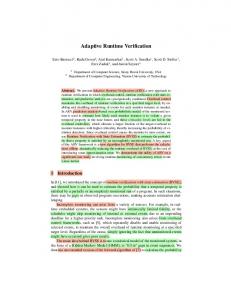
Fig. 5. Main properties of the logics studied in this paper. The numbers in brackets refer to the remark stating the result.

7

Conclusion

In this paper we study several variants of linear temporal logics in the context of runtime verification. In runtime verification, we are faced with an incrementally expanding prefix of an unknown infinite trace representing an execution of the underlying system, for which we have to decide whether a property expressed in a linear temporal logic holds. Thus, when considering logics for runtime verification, we look for linear temporal logics interpreted over finite traces, with a semantics reflecting that of LTL over infinite traces in a suitable manner. To this end, we have recalled three existing linear temporal logics interpreted over finite traces, namely, FLTL [MP95], LTL∓ [EFH+ 03], and LTL3 [BLS06] and elaborated on their properties, for example, which equivalences of formulae hold in the respective logic and how they compare to those in LTL. Moreover, we established four maxims that we consider essential for a linear temporal logic aimed for runtime verification: (1) Existential next requires the inclusion of a strong next operator. (2) Complementation by negation requires that a negated formula evaluates to the complemented and different truth value. (3) Impartiality requires that a finite trace is not evaluated to ⊤ (⊥) if there still exists an infinite continuation leading to another verdict. (4) Anticipation requires that once every infinite continuation of a finite trace leads to the same verdict, then the finite trace evaluates to this very same verdict. We analysed FLTL, LTL∓ , and LTL3 with respect to these maxims and learnt that none of them satisfies all four of them. This lead us to the introduction of RV-LTL, whose semantics combines ideas present in LTL3 as well as FLTL. The semantics of RV-LTL indicates whether a finite word describes a system behaviour which either (1) satisfies the monitored property, (2) violates the property, (3) will presumably violate the property, or (4) will presumably conform to the property in the future, once the system has stabilised. Using these truth values, we resolved the ugly situation of facing an invariably inconclusive verdict in verifying a system at runtime: As long as the final verdict depends on future events, an RV-LTL-based monitor displays a presumably true valuation—if no unanswered request is pending—and presumably false otherwise. 21

We analysed some basic properties of RV-LTL and especially verified that RV-LTL acts on our four maxims. To turn RV-LTL in a practically applicable device for runtime verification, we developed a monitor generation procedure that relies on corresponding monitor constructions for FLTL and LTL3 . A summarising comparison of the logics studied in this paper is shown in Figure 5.

References [ABLS05] Oliver Arafat, Andreas Bauer, Martin Leucker, and Christian Schallhart. Runtime verification revisited. Technical Report TUM-I0518, Technische Universit¨ at M¨ unchen, 2005. [Bel77] Nuel D. Belnap. A useful four-valued logic. In Gunnar Epstein and J. Michael Dunn, editors, Modern uses of multiple-valued logic, pages 8–37. Reidel, Dordrecht, NL, 1977. [BLS06] Andreas Bauer, Martin Leucker, and Christian Schallhart. Monitoring of real-time properties. In FSTTCS, volume 4337 of LNCS, December 2006. [BLS07a] Andreas Bauer, Martin Leucker, and Christian Schallhart. The good, the bad, and the ugly—but how ugly is ugly? In Proceedings of the 7th International Workshop on Runtime Verification (RV’07), volume 4839 of Lecture Notes in Computer Science, pages 126–138, Vancouver, Canada, December 2007. Springer-Verlag. [BLS07b] Andreas Bauer, Martin Leucker, and Christian Schallhart. Runtime Verification for LTL and TLTL. Transactions on Software Engineering (TSE), 2007. submitted, preliminary version available as Tech. Rep. TUM-I0724. [dR05] Marcelo d’Amorim and Grigore Rosu. Efficient monitoring of omega-languages. In Kousha Etessami and Sriram K. Rajamani, editors, CAV, volume 3576 of LNCS, pages 364–378, 2005. [Dru00] Doron Drusinsky. The temporal rover and the ATG rover. In Klaus Havelund, John Penix, and Willem Visser, editors, SPIN, volume 1885 of LNCS, pages 323–330, 2000. [EFH+ 03] Cindy Eisner, Dana Fisman, John Havlicek, Yoad Lustig, Anthony McIsaac, and David Van Campenhout. Reasoning with temporal logic on truncated paths. In CAV, volume 2725 of LNCS, pages 27–39, 2003. [GH01a] Dimitra Giannakopoulou and Klaus Havelund. Automata-based verification of temporal properties on running programs. In ASE, pages 412–416. IEEE Computer Society, 2001. [GH01b] Dimitra Giannakopoulou and Klaus Havelund. Runtime analysis of linear temporal logic specifications. Technical Report 01.21, RIACS/USRA, 2001. [Hop71] J.E. Hopcroft. An n log n algorithm for minimizing states in a finite automaton. Theory of Machines and Computation, pages 189–196, 1971. [HR01a] Klaus Havelund and Grigore Rosu. Monitoring Java Programs with Java PathExplorer. ENTCS, 55(2), 2001. [HR01b] Klaus Havelund and Grigore Rosu. Monitoring programs using rewriting. In ASE, page 135. IEEE Computer Society, 2001. [HR02] Klaus Havelund and Grigore Rosu. Synthesizing Monitors for Safety Properties. In TACAS, volume 2280 of LNCS, pages 342–356, 2002. [Kam68] H. W. Kamp. Tense Logic and the Theory of Linear Order. PhD thesis, University of California, Los Angeles, 1968. [KV01] Orna Kupferman and Moshe Y. Vardi. Model checking of safety properties. Form. Methods Syst. Des., 19(3):291–314, 2001. [MP95] Zohar Manna and Amir Pnueli. Temporal Verification of Reactive Systems: Safety. Springer, New York, 1995. [Pnu77] Amir Pnueli. The temporal logic of programs. In FOCS, pages 46–57. IEEE Computer Society Press, October 31–November 2 1977. [RB06] Grigore Rosu and Saddek Bensalem. Allen linear (interval) temporal logic - translation to LTL and monitor synthesis. In CAV, volume 4144 of LNCS, pages 263–277, 2006.

22

[SB05] [Var96] [VW86]

Volker Stolz and Eric Bodden. Temporal Assertions using AspectJ. In RV, volume 144/4 of ENTCS, 2005. Moshe Y. Vardi. An automata-theoretic approach to linear temporal logic, 1996. M. Y. Vardi and P. Wolper. An automata-theoretic approach to automatic program verification. In LICS, pages 332–345, 1986.

23