comparing model development in discrete event simulation and ...

Proceedings of the 2009 Winter Simulation Conference M. D. Rossetti, R. R. Hill, B. Johansson, A. Dunkin and R. G. Ingalls, eds.

COMPARING MODEL DEVELOPMENT IN DISCRETE EVENT SIMULATION AND SYSTEM DYNAMICS Antuela A. Tako Stewart Robinson Warwick Business School University of Warwick Coventry, CV4 7AL, United Kingdom ABSTRACT This paper provides an empirical study on the comparison of model building in Discrete-Event Simulation (DES) and System Dynamics (SD). Verbal Protocol Analysis (VPA) is used to study the model building process of ten expert modellers (5 SD and 5 DES). Participants are asked to build a simulation model based on a prison population case study and to think aloud while modelling. The generated verbal protocols are divided into 7 modelling topics: problem structuring, conceptual modelling, data inputs, model coding, validation & verification, results & experimentation and implementation and then analyzed. Our results suggest that all modellers switch between modelling topics, however DES modellers follow a more linear progression compared to SD modellers. DES modellers focus significantly more on model coding and verification & validation, whereas SD modellers on conceptual modelling. This quantitative analysis of the processes followed by expert modellers contributes towards the comparison of DES and SD modelling. 1

INTRODUCTION

Discrete-Event Simulation (DES) and System Dynamics (SD) are two established simulation approaches in Operational Research (OR). Both simulation approaches started and evolved almost simultaneously with the advent of computers, but very little communication existed between these fields (Sweetser 1999, Lane 2000, Morecroft and Robinson 2005). This is however, changing at present with more DES or SD academics and practitioners showing an interest to enter the other world (Morecroft and Robinson 2005). Work on the comparison of the two simulation approaches is limited. The comparisons made are mostly opinion-based, derived from the authors’ personal opinions and field of expertise (Brailsford and Hilton 2001, Morecroft and Robinson 2005). Hence, little understanding exists regarding the differences and similarities between the two simulation approaches, let alone understanding when should one approach be used instead of the other. In an attempt to assist towards this lack of objectivity in the comparisons found in the literature, this paper presents an empirical study on the comparison of DES and SD model building process. 1.1

DES and SD

Some key fundamental differences exist between DES and SD, which are derived from the underlying principles of each simulation approach and software used. These are briefly considered in this section, however, the technical differences between them are not the scope of the current paper. DES models systems as a network of queues and activities, where state changes occur at discrete points of time, whereas SD models consist of a system of stocks and flows where continuous state changes occur over time (Brailsford and Hilton 2001). In DES the objects (entities) are individually represented and can be tracked through the system. Specific attributes are assigned to each entity and determine what happens to them throughout the simulation. On the other hand, in SD entities are presented as a continuous quantity. In DES state changes occur at discrete points of time, while in SD state changes happen continuously at small segments of time (Δt). Specific entities cannot be followed throughout the system. DES models are stochastic in nature with randomness incorporated through the use of statistical distributions. SD models are generally deterministic and variables usually represent average values. Despite the differences listed, it is claimed that the objective of models in both simulation approaches is to understand how systems behave over time and to compare their performance under different conditions (Sweetser 1999).

978-1-4244-5771-7/09/$26.00 ©2009 IEEE

979

Tako and Robinson 1.2

Scope of The Current Paper

The work described in this paper compares DES and SD simulation modelling as observed during the model development process. The comparison is based on the processes followed by expert modellers during a simulation modelling task. Individual modelling sessions are developed with 10 expert modellers (5 DES and 5 SD), who are provided with a case study and asked to build simulation models. The research method used is that of Verbal Protocol Analysis (VPA), which involves a detailed analysis of the cognitive processes that take place when individual participants undertake a problem-solving exercise. This study provides a quantitative analysis that compares the modelling process followed by the DES and SD modellers. The underlying aim is to bring closer the two fields of simulation, with a view to creating a common basis of understanding. The paper is outlined as follows. It starts with a review of the existing literature on the comparison of DES and SD, followed by a description of the study undertaken, where the case study and the research method used (VPA), are described. We then present the quantitative results of the study, based on observations from 10 modelling sessions. Finally, we discuss the main findings and the limitations of the current study. 2

EXISTING WORK ON THE COMPARISON OF DES AND SD

In this section, the existing literature on the comparison of the two simulation techniques DES and SD is reviewed. First, an overview of the main comparison studies found is provided, to be continued with more specific views expressed about the model building process followed in each approach. 2.1

Overview of DES and SD Comparison Studies

Existing work on the comparison of DES and SD is scarce. In the few studies found, comparisons tend to be biased towards either the DES or SD approach. The views expressed consist mainly of the authors’ personal opinions based on their own area of expertise (Brailsford and Hilton 2001). Whilst one might suppose that this makes them natural antagonists it can be argued that they complement each other (Morecroft and Robinson 2005). The opinions expressed regarding the comparison of DES and SD are built around the practice of model development, modeling philosophy and the use of respective models in practice. A long list with the views expressed can be compiled, however due to space limitations only some examples of differences are provided (Table 1), in order to give the reader an idea. Table 1: Examples of views expressed in the literature regarding the comparison of DES and SD modeling Aspects compared Nature of problems modelled Feedback effects System representation Complexity Data inputs Randomness Validation Model results

DES Tactical/operational.

SD Strategic.

Author (s) Sweetser 1999, Lane 2000

Models open loop structures – less interested in feedback. Analytic view. Narrow focus with great complexity & detail. Quantitative based on concrete processes. Use of random variables (statistical distributions). Black-box approach. Provides statistically valid estimates of system performance.

Models causal relationships and feedback effects. Holistic view. Wider focus, general & abstract systems. Quantitative & qualitative, use of anecdotal data. Stochastic features less often used (averages of variables). White-box approach. Provides a full picture (qualitative & quantitative) of system performance.

Coyle 1985, Sweetser 1999, Brailsford and Hilton, 2001 Baines et al.1998, Lane 2000 Lane 2000 Sweetser 1999, Brailsford and Hilton 2001 Meadows 1980 Lane 2000 Meadows 1980, Mak 1993

The main comparison studies are now briefly considered in a chronological order. First, Coyle (1985) comes into the discussion from a SD perspective, while considering ways to model discrete events in a SD environment. His comparison focuses on two aspects: randomness existing in DES modelling and the model structure, where it is claimed that open-loop versus closed loop systems are represented in SD and DES respectively. In her doctoral thesis, Mak (1993) studies how DES activity cycle diagrams can be converted into SD stock and flow diagrams. Mak also presents a list of fundamental differences between DES and SD modelling.

980

Tako and Robinson Coming from a consultancy background, Sweetser (1999) provides a comparison based on the established modelling practice and the conceptual views of modellers in each area. He ends by comparing DES and SD conceptual models of a production process. Brailsford & Hilton (2001) compare DES and SD in the context of health care modelling. The authors compare the main characteristics and the application of the two approaches, based on two specific health-care studies presented (one in SD and the other in DES) and on their own experience as modellers. They conclude with a presentation of the technical differences between the two approaches, providing a list of criteria when each approach is more appropriate. Lane (2000) gives a thorough comparison between DES and SD, focusing on the conceptual differences. His discussion is again based on his personal experience as a system dynamicist. Lane considers three modes of discourse, where it is argued that DES and SD can be presented as different or similar based on the position taken (the mode of discourse). At the end, Lane provides a list of conceptual differences, taking a mutual approach. However, Morecroft and Robinson (2005), disagree with some of the statements made. Theirs is the first study that undertakes an empirical comparison using a common fishery model. The authors build a step-by-step simulation model, using DES (Robinson) and SD (Morecroft) modelling. However, one could claim the existence of bias, as the two modellers were aware of each other’s views on simulation modelling. An empirical study on the comparison of DES and SD from the users’ point of view was carried out by Tako and Robinson (2009). The authors found that users’ perceptions of two simple DES and SD models were not significantly different. So far, no study has been yet identified that provides an unbiased empirical account on the comparison of the DES and SD model development process. 2.2

DES and SD Model Development Process

Considering the model development process, as suggested in DES and SD textbooks teaching the art of simulation modelling, one can identify similarities especially in terms of the stages involved. This is depicted in diagrams a and b in Figure 1. It is clear that the main stages followed are equivalent to generic OR modelling (Hillier and Lieberman 1990, Oral and Kettani 1993, Willemain 1995), which are as follows: • Problem definition • Conceptual modelling • Model coding • Model validity • Model results and experimentation • Implementation and learning a)

b)

Figure 1: The DES (a) and SD (b) modelling process, where a) is based on (Robinson 2004) and b) on (Sterman 2000) Looking more closely at views expressed regarding the model building process followed, it is mentioned that in DES modelling emphasis is given to the development of the model on the computer (model coding). Baines et al. (1998) completed an experimental study of various modelling techniques, among others DES and SD, and their ability to evaluate manufacturing strategies. The authors commented on the time taken in building the DES model. The time taken in model building was considerably longer compared to SD and other modelling techniques. Furthermore, Artamonov (2002) developed two

981

Tako and Robinson equivalent DES and SD models of the beer distribution game model (Senge 1990) and commented on the difficulty involved in coding the model on the computer. He found the development of the model on the computer more difficult in the case of the DES approach, whereas, the development of the SD model was less troublesome. One possible explanation given by Baines et al (1998) is the fact that DES encourages the construction of a more lifelike representation of the real system compared to the other techniques, which consequently results in a more detailed and complex model. On the other hand, in SD modelling emphasis is given to understanding the system structure and the dynamic tendencies involved. Consequently, Meadows (1980) highlights that system dynamicists spend the most amount of simulation modelling time specifying the model structure. The specification of the model structure consists of the representation of the causal relationships that generate the dynamic behaviour of the system. This is equivalent to the development of the conceptual model. Another important feature of DES and SD modelling is the iterative nature of the modelling process. In both, DES and SD textbooks, it is highlighted that simulation modelling involves a number of repetitions and iterations (Randers 1980, Sterman 2000, Pidd 2004, Robinson 2004). This is again depicted in Figure 1, where a similarly iterative cycle is depicted for both DES (part a) and SD (part b) modelling. It is clear that the sequence between simulation modelling stages does not follow a linear progression from problem definition to conceptual modelling, model coding, etc. Regardless of the modeller’s experience, a number of repetitions occur from the creation of the first simulation model. So long as the number of iterations remains reasonable, these are in fact quite desirable (Randers 1980). Based on the above, the main aspects considered about the simulation model development process in DES and SD, consist of the amount of attention paid to the different stages during modelling, the sequence of modelling stages followed and the pattern of iterations followed among the different modelling stages. 3

THE STUDY

The overall objective of this study is to empirically compare the behaviour of expert modellers while undertaking a DES and SD modelling task. We believe that DES and SD modellers think differently during the model building process. Therefore, it is expected that while observing expert modellers building simulation models, these differences become evident. The authors use qualitative textual analysis and perform both quantitative and qualitative analyses of the resulting data to identify these differences. The current paper focuses only on the quantitative analysis undertaken, which aims to compare DES and SD modellers’ thinking, analysing the modelling stages they think about while building simulation models. The aim is to compare the model development process followed by DES and SD modellers regarding: the attention paid to different modelling stages, the sequence of modelling stages followed and the pattern of iterations. In this section the study undertaken is explained. First, the case study used is briefly described, followed by a brief introduction to the research method, Verbal Protocol Analysis (VPA). Next, we report on the profile of the participants involved in the study and the coding process carried out. 3.1

The Case Study

A suitable case study for the purposes of this research needs to be sufficiently simple to enable the development of a simulation model, which can be built in a short period of time (60-90 minutes). In addition, a suitable case study needs to accommodate the development of models using both simulation techniques, so that the specific features of each technique (randomness in DES vs. deterministic models in SD, the aggregated presentation of entities in SD vs. the individual representation of entities in DES, etc.) are present in the models built. Among others, the authors were interested to see how the same aspects of the problem would be represented with each simulation approach (e.g. the feedback effects). After considering a number of possible contexts, the prison population problem was selected. The prison population case study, where prisoners enter prison initially as first time offenders and are then released or return back to prison as recidivists can be represented by simple simulation models using both DES and SD. Furthermore, both approaches have previously been used for modelling the prison population system. DES models of the prison population have been developed by Kwak et al. (1984), Cox et al. (1978), Korporaal et al. (2000), and SD models have been developed in Bard (1978), and McKelvie et al. (2007), while the UK prison population model by Grove et al. (1998) is a flow model analogous to an SD model. Hence, the UK prison population case study is considered suitable for this research. The UK prison population example used in this research is based on Grove et al. (1998). The case study starts with a brief introduction to the prison population problem with particular attention to the issue of overcrowded prisons. Descriptions of the reasons for, and impacts of, the problem are provided. The figures and facts used in the case study are mostly based on reality, but slightly adapted for the purposes of the research. Two types of prisoners are involved, petty and serious offenders. There is already an initial number of prisoners in the system (76,000). Offenders enter the system as first time offenders and receive a sentence depending on the type of offence. Petty offenders enter the system at a higher rate, on average 3,000 people/year vs. 650 people/year for serious offenders, but receive a shorter sentence length, on average 5 years vs. 20

982

Tako and Robinson years for serious offenders. After serving time in prison the offenders are released. A proportion of the released prisoners reoffend and go back to jail (recidivists) after on average 2 years. Petty prisoners are more likely to re-offend. However, these numbers were intentionally not given to the modellers, to test whether they would make their own assumptions or ask for further data. For more details on the case study, the reader is referred to (Tako and Robinson 2009). In order to solve the problem of overcrowded prisons, two possible scenarios are provided, either to increase the current prison capacity and so facilitate the introduction of stiffer rules, or the alternative of reducing the size of the prison population by introducing alternatives to jail and/or enhancing the social support provided to prisoners. The task for participating modellers was to create a simulation model, which would be used as a decision-making tool by policy makers. 3.2

Verbal Protocol Analysis (VPA)

VPA is a research method derived from psychology. It requires the subjects to ‘think aloud’ when making decisions or judgements during a problem-solving exercise. It relies on the participants’ generated verbal protocols in order to understand in detail the mechanisms and the internal structure of cognitive processes that take place (Ericsson and Simon 1984). Therefore, VPA as a process tracing method provides access to the activities that occur between the onset of a stimulus (case study) and the eventual response to it (model building) (Ericsson and Simon 1984, Todd and Benbasat 1987). Willemain (1994, 1995) was the first to use it in Operational Research (OR) to document the thought processes of OR experts while building models. VPA is considered to be an effective method for the comparison of the DES and SD model building process. It is useful because of the richness of information and the live accounts it provides on the experts’ modelling process. Another potential research method would have been to observe real-life simulation projects, using DES and SD. However, for a valid comparison it is necessary to have comparable modelling situations, which would require two potential real life modelling projects of equivalent problem situations. This was not deemed feasible. We also considered running interviews with modellers from the DES and SD field. Given that the overall aim of this research is to get beyond opinions and to get an empirical view about model building, one can claim that modellers’ reflections may not reflect correctly the processes followed during model building and it would thus not represent a full picture of model building. Hence, interviews were not considered appropriate either. VPA on the other hand, can capture modellers’ thoughts in practical modelling sessions in a controlled experimental environment, using a common stimulus – case study. Protocol analysis as a technique has its own limitations. The verbal reports may omit important data (Willemain 1995) because the experts being under observation may not behave as they normally would. The modellers are asked to work alone and this way of modelling may not reflect their usual practice of model building, where they would interact with the client, colleagues, etc. In addition, there is the risk that participants do not ‘verbalize’ their actual thoughts, but are only ‘explaining’. To overcome this and to ensure that the experts speak their thoughts aloud, short verbalization exercises, based on Ericsson and Simon (1984) were run at the beginning of the sessions. 3.3

The VPA Sessions

The subjects involved in this study were provided with the prison population case study at the start of the VPA session and were asked to build simulation models based on it using their preferred simulation approach. During the modelling process experts were asked to ‘think aloud’ as they model. The researcher (Tako) sat in the same room, but social interaction with the subjects was limited. She only intervened in the case that participants stopped talking for more than 20 seconds to tell them to “keep talking”. The researcher was also answering explanatory questions and provided participants with additional data inputs (if they asked for) and also prompted them to build a model on the computer in the case when they did not do so by their own initiative. The modelling sessions were held in an office environment with each individual participant. The sessions lasted approximately 60-90 minutes. The participants had access to writing paper and a computer with relevant simulation software (e.g. Simul8, Vensim, Witness, Powersim, etc.), among which they could chose based on their modelling experience. The protocols were recorded on audio tape and then transcribed. 3.4

The Subjects

The subjects involved in the modelling sessions were 10 simulation experts in DES and SD modelling, 5 in each area. The sample size of 10 participants is considered reasonable, although a larger sample would be better. According to Todd and Benbasat (1987), due to the richness of data found in one protocol, VPA samples tend to be small, between two to twenty. For reasons of confidentiality participants’ names are not revealed. In order to distinguish each participant we use the symbol DES or SD, according to the simulation technique used, followed by a number. So DES modellers are called DES1,

983

Tako and Robinson DES2, DES3, DES4 and DES5, while SD subjects SD1, SD2, SD3, SD4 and SD5. All participants use simulation modelling (DES and SD) as part of their work, most of them holding consultant posts in different organizations. The companies they come from are established simulation software companies or consultancy companies based in the UK. The two groups of experts in DES and SD modelling had a mixture of backgrounds, having completed either doctorates or masters’ degrees in engineering, computer science, Operational Research or hold MBAs. Their experience in simulation modelling ranges from at least 6 years up to 19 years. They boast an extensive experience of modelling in areas such as: NHS, criminal justice, food & drinks sector, supply chain, etc. Participants were given the option to choose their preferred simulation software, resulting in different modellers choosing different software. This enables the elimination of bias related to using only one simulation software. 3.5

The Coding Process

A coding scheme was designed in order to identify what the modellers were thinking about in the context of simulation model building. The coding scheme was devised following the stages of typical DES and SD simulation projects, based on Robinson (2004), Law (2007), (Sterman 2000) and (Randers 1980). Each modelling topic has been defined in the form of questions corresponding to the modelling stage considered. The modelling topics and their definitions are as follows: 1. Problem structuring: What is the problem? What are the objectives of the project? 2. Conceptual modelling: Is a conceptual diagram drawn? What are the parts of the model? What should be included in the model? How to represent people? What variables are defined? 3. Model coding: What is the modeller entering on the screen? How is the initial condition of the system modelled? What units (time or measuring) are used? Does the modeller refer to documentation? How to model the user interface? 4. Data inputs: Do modellers refer to data inputs? How are the already provided data used? Are modellers interested in randomness? How are missing data derived? 5. Model results & experimentation: What are the results of the model? What sort of results the modeller is interested in? What scenarios are run? 6. Implementation: How will the findings be used? What learning is achieved? 7. Verification &Validation: Is the model working as intended? Are the results correct? How is the model tested? Why is the model not working? The coding process starts with the definition of a coding scheme. As the modelling sessions were completed the recorded information in a verbal protocol was transcribed. Then the verbal protocols were divided into episodes or ‘thought’ fragments, where each fragment is the smallest unit of data meaningful to the research context. Then each episode was coded into one of the 7 modelling topics or an ‘other’ category for verbalisations that were not related to the modelling task. Some episodes, however, referred simultaneously to 2 modelling topics and, therefore, were given two modelling topics. Regarding the nature of the coding process followed, a mix of top-down and bottom-up approach to coding was taken (Ericsson and Simon 1984, Patrick and James 2004). A theoretical base was already established (the initially defined modelling topics), which enabled a top-down approach. Throughout the various checks of the coded protocols undertaken, the coding categories were further re-defined through a bottom-up approach. Coding was an iterative process, where the coding scheme was refined as the researchers went through more protocols. This was more prevalent while analysing the protocols obtained from the pilot study, however, even during the coding of the main protocols, some changes were still made. The transcripts were coded manually using a standard word processor. According to Willemain (1995), the coding process requires attention to the context a phrase is used in and, therefore, subjectivity in the interpretation of the scripts is unavoidable. In order to deal with subjectivity, multiple independent codings were undertaken in two phases. In the first stage, one of the researchers (Tako) coded the transcripts twice with a gap of 3 months between codings. Overall, a 93% agreement between the two sets of coding was achieved, which was considered acceptable. The differences were examined and a combined coding was reached. Next, the coded transcripts with the combined codes were further blind checked by a third party, knowledgeable in OR modelling and simulation. In the cases where the coding did not agree, the researcher who undertook the coding and the third party discussed the differences and re-examined the episodes to arrive at a consensus coding. Overall, a 90% agreement between the two codings was achieved. A final examination of the coded transcripts was undertaken by the researcher to check the consistency of the coded episodes. Some more changes were made to the definition of modelling topics, but these were fairly minor. The results from the coded protocols are now presented and discussed.

984

Tako and Robinson 4

STUDY RESULTS

This section presents the results of a quantitative analysis of 10 coded protocols. The data represent a quantitative description of participants’ modelling behaviour, exploring the distribution of attention to modelling topics, the sequence of modelling stages during the model building exercise and the pattern of iterations followed among topics. The findings from each analysis follow. 4.1

Attention Paid to Modelling Topics

In order to explore the distribution of attention by modelling topic, the number of words articulated is considered a suitable measure of the amount of verbalisation by the expert modellers. In turn, this is used to indicate the spread of modellers’ attention to the different modelling topics. The average number of words for the DES and SD protocols by modelling topic is compared in order to establish significant differences between the two groups. Figure 2 shows the number of words verbalised by modelling topic by the two groups of modellers. Comparing the total number of words verbalised in the overall DES and SD protocols an average difference of 1,751 words is identified, suggesting that DES modellers verbalise more than SD modellers. The equivalent box plots in Figure 2 (bottom), show that while the medians of words verbalised are close for the DES and SD modellers, there is a bigger variation in the total number of words verbalised by the DES modellers. Considering each specific modelling topic, the biggest differences between the DES and SD protocols, can be identified with regards to model coding, verification & validation and conceptual modelling (Figure 2). This suggests that DES modellers spend more effort in coding the model on the computer and testing it, while SD modellers spend more effort in conceptualising the mental model.

Figure 2: Box and whiskers plot of DES and SD modellers’ verbalisations by modelling topic In order to test the significance of the differences identified, the Kolmogorov-Smirnov test is used as a nonparametric alternative to the t-test for two independent samples when it is believed that the hypothesis of normality does not hold (Sheskin 2007). In this case, only 5 data points (word count for each modeller) are collected from the two groups of modellers (DES and SD). Due to the small sample size and the fact that count data is inherently not normal, it is considered that the assumption of normality is violated. The null hypothesis for the Kolmogorov-Smirnov test assumes that the verbalisations of the DES modellers follow the same distribution as the verbalisations of the SD modellers. The alternative hypothesis is that the data do not come from the same distribution. This test compares the cumulative probability distributions of the number of words verbalised by the modellers in the DES and SD groups. The statistical tests performed indicate significant differences, at a 5% level, in the amount of DES and SD modellers’ verbalisations for the three modelling topics: conceptual modelling, model coding and verification & validation (Table 2). This suggests that DES modellers verbalise more with respect to model coding and verification & validation and thus spend

985

Tako and Robinson more effort on these modelling topics compared to SD modellers. SD modellers verbalise more on conceptual modelling. In addition, the total verbalisations of the two groups of modellers are not found to be significantly different. Furthermore, a chisquare test comparing the distribution of the number of words verbalised among the modelling topics for the two groups of modellers reveals that the distribution of attention among modelling topics is not the same (from the calculations, the chisquare value found is 6,892.89 greater than the critical value of χ 2 0.05, 6 = 12.59 ). Table 2: The results of the Kolmogorov-Smirnov test comparing the DES and SD modellers’ verbalisations for 7 modelling topics and the total protocols. The significant differences are highlighted, based on the comparison of the greater vertical distance M to the critical value =0.8 (Sheskin, 2007). M

Modelling topic P roblem s tructuring C onceptual modelling Model coding D ata inputs Verification & Validation R es ults & experimentation Implementation T otal protocol

4.2

0.6 0.8 0.8 0.6 1 0.4 0.4 0.4

Differenc es in verbalis ations ?        

The Sequence of Modelling Stages

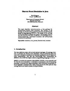
This section focuses on the progression of modellers’ attention during a simulation model development task using time line plots. Timeline plots represent the modelling topic modellers think about and when during a simulation modelling task (Willemain 1995, Willemain and Powell 2006). A timeline plot is created for each of the 10 verbal protocols. It consists of a matched set of 7 timelines showing which of the seven modelling topics the modeller is attending to throughout the duration of the modelling exercise. The vertical axis takes three values, 1 when the specific modelling topic is attended to by the modeller, 0.5 when the modelling topic and another have been attended to and 0 when the modelling topic is not mentioned. The horizontal axis represents the proportion of the verbal protocol, from 0% to 100% of the number of words. The proportion of the verbal protocol is counted as the fraction of the cumulative number of words for each consecutive episode over the total number of words in that protocol, expressed as a percentage. Figures 3 and 4 show a sample of timeline plots for DES1 and DES5, and SD1 and SD3 respectively. Due to space limitations only 4 timeline plots are included. It should be however noted that these are representative of most timeline plots obtained in this study, apart from DES3 and SD5. The former modeller did not complete the model due to difficulties encountered with the large number of attributes and population size. The latter was reluctant to build a model on the computer and so attended to model coding only at the end of the protocol, after being prompted by the researcher. Timeline DES1

Timeline DES5

Problem structuring

Problem structuring

Conceptual modelling

Conceptual modelling

Model coding

Model coding

7

6

5

4

Data Inputs

Data Inputs

Valid & Verification

Valid & Verification

Results & Experimentation

Results & Experimentation1

Implementation

Implementation

3

2

0

0

% of total words

1

0

Figure 3: Timeline plots for 2 DES protocols (DES1 and DES5)

986

% of total words

1

Tako and Robinson Observing the DES and SD timeline plots it is obvious that modellers switched frequently their attention among topics. Similar patterns of behaviour were observed by Willemain (1995) in his study where expert modellers where asked to build models of a generic OR problem. Looking at the overall tendencies in the DES and SD timeline plots, it appears that the DES protocols might follow a more linear progression in the sequence of modelling topics. Meanwhile, in the SD protocols, modellers’ attention appears to be more scattered throughout the model building session (Figure 4). The transition of attention between modelling topics is further explored in section 4.3. Timeline SD1

7

Problem structuring

Timeline SD3 Problem structuring

6

Conceptual modelling Model coding

Conceptual modelling

5

Model coding 4

Data Inputs

Data Inputs 3

Valid & Verification

7

6

5

4

3

Valid & Verification

2

2

Results & experimentation

Results & Experimentation

Implementation

Implementation

1

1

0

0

0

% of total words

1

% of total words

0

1

Figure 4: Timeline plots for 2 SD protocols (SD1 and SD3) 4.3

Pattern of Iterations Among Topics

In this section the iterations among modelling topics is explored using transition matrices, with a view to further understanding the pattern of iterations followed by DES and SD modellers. A transition matrix represents the cross-tabulation of the sequence of attention between successive pairs of episodes in a protocol. The total number of transitions occurring in the combined DES and SD protocols is displayed in Figure 5. It is observed that DES and SD modellers switched their attention from one topic to another almost to the same extent (505 times for DES modellers and 507 times for SD modellers). In order to explore the dominance of modellers’ thinking, the cells in the transition matrices have been highlighted according to the number of transitions counted. The darkest colours, in this case purple and dark blue, represent the transitions that occur most frequently. DES Transition matrix PS CM PS 0 CM 2 MC 1 DI 0 V&V 2 R&E 3 Impl 1 Totals 9

MC 1 0 37 21 11 4 0 74

SD Transition matrix PS CM PS 0 8 CM 6 0 MC 4 37 DI 3 40 V&V 1 10 R&E 5 21 Impl 0 1 Totals 19 117

DI 2 42 0 70 58 12 1 185

MC

V&V 4 21 75 0 9 5 0 114

DI 1 44 0 50 17 21 2 135

0 6 62 15 0 7 0 90 V&V

4 41 46 0 11 13 0 115

0 7 22 8 0 11 0 48

R&E

Impl

3 6 10 2 10 0 0 31 R&E 8 16 24 10 9 0 1 68

0 0 0 0 0 2 0 2

Totals 10 77 185 108 90 33 2 505

0 2 2 0 0 1 0 5

Totals 21 116 135 111 48 72 4 507

Impl

0 1--10 11--20 21--40 40+

Figure 5: Comparative view of the transition matrices for the combined DES and SD protocols, where each cell has been colour-coded depending on the number of transitions

987

Tako and Robinson The main observations made based on the DES and SD transition matrices are: • Model coding is the topic DES modellers return to most often (185). Similarly, SD modelers return mostly to model coding. • The modelling topics that DES modellers alternate between most often are: conceptual modelling, model coding, data inputs and verification & validation (shown by the blue highlighted cells in DES transition matrix Figure 5). • SD modellers alternate mostly in a loop between conceptual modelling, model coding and data inputs. These transitions determine the dominant loop in their thinking process (blue highlighted cells in SD transition matrix Figure 5). • Comparing the two transition matrices, the pattern of the transitions for SD modelers follows a more horizontal progression, while a diagonal progression towards the right-hand bottom end of the matrix for DES modellers. An indication of a more linear progression is observed for DES modelers compared to SD modellers. This indication of linearity is further verified using the total number of transitions of attention for the parallel linear strips in the two transition matrices (DES and SD). The cells in the transition matrices in Figure 5 have been colour-coded, where one cell follows the next cell down on the right (part a, Figure 6). So 8 linear strips with different colours have been created, for which the total number of transitions is counted (part b, Figure 6). In the case of absolute linear thinking, it would be expected that all transitions would be concentrated in the central (blue) strip. However, this is not the case with any of the DES or SD protocols. Nevertheless, the total number of transitions for all 8 linear strips provides an indication of the extent of linearity involved. The further away a strip is from the central strip, the fewer transitions are expected in order to convey linearity. The total number of transitions per linear strip are compared for the DES and SD protocols (part b, Figure 6).

a)

PS CM MC DI V&V R&E Impl Totals

Transition matrix - Total DES PS CM MC 0 1 2 0 1 37 0 21 2 11 3 4 1 0 9 74

2 42 0 70 58 12 1 185

Topic transition - Total SD PS CM MC 0 8 6 0 4 37 3 40 1 10 5 21 0 1 19 117

1 44 0 50 17 21 2 135

PS CM MC DI V&V R&E Impl Totals

DI

DI

4 21 75 0 9 5 0 114

4 41 46 0 11 13 0 115

V&V

V&V

0 6 62 15 0 7 0 90

0 7 22 8 0 11 0 48

R&E

R&E

3 6 10 2 10 0 0 31

8 16 24 10 9 0 1 68

Impl

Impl

Colour code

0 0 0 0 0 2 0 2

0 2 2 0 0 1 0 5

b)

DES 145 125 87 85 20 23 6 7

SD 116 116 74 74 35 34 18 24

Figure 6: Total number of transitions per linear strip in the DES and SD transition matrices For the DES modellers the higher numbers are at the top of the table, representing the most central strips. This implies that the transition of attention for the DES modellers focuses mainly in the more central strips in the matrix. For the SD modellers, while the higher totals of transitions still correspond to the most central strips, looking comparatively further down in the columns in Table 6b, higher totals are observed for the further away strips compared to DES modellers. The highest totals in the further away strips suggest that the SD modellers switched their attention in a more cyclical pattern compared to the DES modellers. Given that an almost equal total number of transitions among topics has been found for DES and SD modellers, it can be concluded that DES modellers’ attention progresses relatively more linearly among modelling topics compared to that of SD modellers. 5

DISCUSSION AND CONCLUDING REMARKS

In summary, the empirical study presented in this paper found the following: 1. DES modellers focus significantly more on model coding and verification & validation of the model, whereas SD modellers concentrate more on conceptual modelling. 2. DES modellers progress more linearly among modelling topics compared to SD modellers. 3. DES and SD modellers follow an iterative modelling process, but their pattern of iteration differs. • DES and SD modellers switch their attention frequently between topics, and almost to the same extent (505 times for DES modellers and 507 for SD modellers) during the model building exercise. • The cyclicality of thinking during the modelling task is more distinctive for SD modellers compared to DES modellers. The modelling process followed by DES and SD modellers was compared by undertaking a quantitative analysis of the verbal protocols. Almost all the modelling sessions resulted in the development of simple DES or SD models of the prison population, where few differences could be identified among them. The results from the analysis of the verbal protocols supported the views expressed in the literature and were on the whole as expected. As with generic OR modelling, both DES and SD follow an iterative modelling process. A new insight gained from this analysis was that DES modellers’ thinking fol-

988

Tako and Robinson lowed a more linear process, whereas for SD modellers it involved more cyclicality. As expected, differences were identified in the attention paid to different modelling stages. The authors believe that this finding is partly a result of the fact that DES modellers naturally tend to pay more attention to model coding and partly because it is inherently harder to code in DES modelling. Clearly, the results are dependent to some extent on the case study used and the modellers selected. Therefore, considerations are made about the limitations of the study and the consequent validity of the findings. Obviously, it should be noted that the findings of this study are based on the researcher’s interpretation of participants’ verbalisations. Subjectivity is involved in the analysis of the protocols, as well as in the choice of the coding scheme. A different researcher might have reached different conclusions (using a different coding scheme with different definitions). In order to deal with subjectivity, the protocols were coded 3 times, involving in one case a third party. Additionally, the current findings are based on the verbalisations obtained from a specific sample of modellers who were chosen based on convenience sampling. The expert modellers who participated in this research were mostly related to one of the two simulation techniques, either DES or SD, but not both. If they had a similar experience of both simulation approaches, the results of this study could have been different. A bigger sample size could have also provided more representative results, however, due to project timescales this was not feasible. In this study only one case study was used, which was considered amenable to both simulation approaches. For future research, the use of more case studies could provide more representative results regarding the differences between the two modelling approaches. Considering the data (verbal protocols) obtained from the modelling sessions implemented, these are derived from artificial laboratory settings, where the modellers at times felt the pressure of time or the pressure of being observed. The task given to the participants was a simple and a quite structured task to ensure completion of the exercise for a limited amount of time. These factors have to some extent affected the smaller amount of verbalisations for modelling topics such as: problem structuring, results & experimentation and implementation. This paper presents a quantitative analysis that compares the behaviour of expert DES and SD modellers when building simulation models. This is the only empirical study that compares the DES and SD model development process based on data gained from experimental exercises involving expert modellers themselves. In this paper, we provide only a quantitative description of expert modellers’ thinking process, analysing the processes that DES and SD modellers think about while building simulation models. This work can ultimately help in the selection of the appropriate simulation approach to model a particular problem situation, albeit specific answers are not provided. The authors, therefore, believe that the findings presented in this paper contribute to the comparison literature. For future research the authors will take this study further with an indepth qualitative analysis of the 10 verbal protocols. The qualitative analysis intends to identify differences in the underlying thought processes between DES and SD expert modellers. ACKNOWLEDGMENTS The authors would like to thank Suchi (Patel) Collingwood for her help with the coding of the protocols, who patiently undertook the third blind check of the ten coded protocols. REFERENCES Artamonov, A. 2002. Discrete-event Simulation vs. System Dynamics: Comparison of Modelling Methods. Warwick Business School, University of Warwick, Coventry. Baines, T. S., D. K. Harrison, J. M. Kay and D. J. Hamblin. 1998. "A consideration of modelling techniques that can be used to evaluate manufacturing strategies " The International Journal of Advanced Manufacturing Technology 14(5): 369375. Bard, J. F. 1978. "The Use of Simulation in Criminal Justice Policy Evaluation." Journal of Criminal Justice 6(2): 99-116. Brailsford, S. and N. Hilton. 2001. A Comparison of Discrete Event Simulation and System Dynamics for Modelling Healthcare Systems. In Proceedings of the 26th meeting of the ORAHS Working Group 2000, ed. J. Riley, pp.18-39. Glasgow, Scotland: Glasgow Caledonian University. Cox, G. B., P. Harrison and C. R. Dightman. 1978. "Computer Simulation of Adult Sentencing Proposals." Evaluation Program Planning 1(4): 297-308. Coyle, R. G. 1985. "Representing Discrete Events in System Dynamics Models: A theoretical Application to Modelling Coal Production." Journal of the Operational Research Society 36(4): 307-318. Ericsson, K. A. and H. A. Simon. 1984. Protocol Analysis: Verbal Reports as Data. Cambridge, MA, MIT Press. Grove, P., J. Macleod and D. Godfrey. 1998. "Forecasting the prison population." OR Insight 11(1). Hillier, F. S. and G. J. Lieberman. 1990. Introduction to Operations Research 5th ed. New York: McGraw-Hill.

989

Tako and Robinson Korporaal, R., A. Ridder, P. Kloprogge and R. Dekker. 2000. "An analytic model for capacity planning of prisons in the Netherlands." Journal of the Operational Research Society 51(11): 1228-1237. Kwak, N. K., P. J. Kuzdrall and M. J. Schniederjans. 1984. "Felony Case Scheduling Policies and Continuances - a Simulation Study." Socio-Economic Planning Sciences 18(1): 37-43. Lane, D. C. 2000. You Just Don't Understand Me: Models of failure and success in the discourse between system dynamics and discrete event simulation. Working paper, 00.34:26: London School of Economics and Political Sciences. Law, A. M. 2007. Simulation modeling and analysis. 4th ed. Boston; London: McGraw-Hill. Mak, H.-Y. 1993. System dynamics and discrete event simulation modelling. PhD thesis, London School of Economics and Political Science, University of London, London. McKelvie, D., S. Hadjipavlou, D. Monk, S. Foster, E. Wolstenholme and D. Todd. 2007. The use of SD methodology to develop services for the assessment and treatment of high risk serious offenders in England and Wales In Proceedings of the 25th International conference of the System Dynamics Society, ed. John Sterman, Rogelio Oliva, Robin S. Langer, Jennifer I. Rowe and Joan M. Yanni, Boston, USA: System Dynamics Society. Meadows, D. H. 1980. The Unavoidable A Priori. Elements of the System Dynamics Methods. Jorgen Randers. Cambridge, Productivity Press. Morecroft, J. D. W. and S. Robinson. 2005. Explaining Puzzling Dynamics: Comparing the Use of System Dynamics and Discrete-Event Simulation. In Proceedings of the 23rd International Conference of the System Dynamics Society, ed. Sterman JD, Repening MP, Langer RS, Rowe JI and Yarni JM, Boston: System Dynamics Society. Morecroft, J. D. W. and S. Robinson. 2005. Explaining Puzzling Dynamics: Comparing the Use of System Dynamics and Discrete-Event Simulation. In In Proceedings of the 23rd International Conference of the System Dynamics Society, ed. Boston: Oral, M. and O. Kettani. 1993. "The facets of the modeling and validation process in operations research." European Journal of Operational Research 66(2): 216-234. Patrick, J. and N. James. 2004. "Process tracing of complex cognitive work tasks." Journal of occupational and organizational psychology 77(2): 259-280. Pidd, M. 2004. Computer simulation in management science. 5th ed. Chichester: Wiley. Randers, J. 1980. Elements of the system dynamics method. Cambridge, Mass., London: M.I.T. Press. Robinson, S. 2004. Simulation: the practice of model development and use. Chichester: Wiley. Senge, P. M. 1990. The Fifth Discipline: The art and practice of the learning organisation. London: Random House. Sheskin, D. J. 2007. Handbook of parametric and nonparametric statistical procedures. 4th ed. Boca Raton: Chapman & Hall/CRC. Sterman, J. 2000. Business dynamics : systems thinking and modeling for a complex world. Boston, London: Irwin/McGrawHill. Sweetser, A. 1999. A Comparison of System Dynamics and Discrete Event Simulation. In Proceedings of 17th International Conference of the System Dynamics Society and 5th Australian & New Zealand Systems Conference, ed. Cavana RY, Vennix JAM, Rouette EAJA, Stevenson-Wright M and Candlish J, Wellington, New Zealand: System Dynamics Society. Tako, A. A. and S. Robinson. 2009. "Comparing discrete-event simulation and system dynamics: Users’ perceptions." Journal of the Operational Research Society 60(3): 296-312. Todd, P. and I. Benbasat. 1987. "Process tracing methods in decision support systems research: exploring the black box." MIS Quarterly 11(4): 493-512. Willemain, T. R. 1994. "Insights on modeling from a dozen experts." Operations Research 42(2): 213-222. Willemain, T. R. 1995. "Model Formulation: What Experts Think about and When." Operations Research 43(6): 916-932. Willemain, T. R. and S. G. Powell. 2006. "How novices formulate models. Part II: a quantitative description of behaviour." Journal of the Operational Research Society 58(10): 1271-1283. AUTHOR BIOGRAPHIES ANTUELA A. TAKO is a Research Fellow in the Operational Research and Management Sciences group a the University of Warwick. She completed her PhD in Simulation at the same University, where she also completed her master studies in Management Science and Operational Research. Her research focuses on simulation and the comparison of different simulation modelling approaches. Key areas of interest are: simulation model development, conceptual modelling and model use. Her e-mail address is .

990

Tako and Robinson STEWART ROBINSON is a Professor of Operational Research at Warwick Business School and Associate Dean for Specialist Masters Programmes. He holds a BSc and PhD in Management Science from Lancaster University. Previously employed in simulation consultancy, he supported the use of simulation in companies throughout Europe and the rest of the world. He is author/co-author of three books on simulation. His research focuses on the practice of simulation model development and use. Key areas of interest are conceptual modeling, model validation, output analysis and modeling human factors in simulation models. His email address is and his Web address is .

991