for biological sequence data (including the Spectrum,. Mismatch, Wildcard, Substitution, Local Alignment and a new Profile-based Local Alignment kernel) on.
Comparing SVM sequence kernels: A protein subcellular localization theme Lynne Davis ab , John Hawkins ab , Stefan Maetschke ab , Mikael Bod´ en b a
ARC Centre for Complex Systems, b School of Information Technology and Electrical Engineering, The University of Queensland, QLD 4072, Australia.
Abstract Kernel-based machine learning algorithms are versatile tools for biological sequence data analysis. Special sequence kernels can endow Support Vector Machines with biological knowledge to perform accurate classification of diverse sequence data. The kernels relative strengths and weaknesses are difficult to evaluate on single data sets. We examine a range of recent kernels tailor-made for biological sequence data (including the Spectrum, Mismatch, Wildcard, Substitution, Local Alignment and a new Profile-based Local Alignment kernel) on a range of classification problems (protein localization in bacteria, peroxisomal protein import signals and sub-nuclear localization). The profile-based local alignment kernel ranks highest, but its computational cost is also higher than for any of the other kernels in contention. The kernels that consistently perform well and tend to produce the most distinct classifications are the Local Alignment, Substitution and Mismatch kernels, suggesting that the exploration of new problem sets should start with these three. 1
Introduction
Support Vector Machines (SVMs) have proved effective on a broad range of biological sequence problems. Examples include the detection of remote protein homologues (Jaakkola, Diekhans & Haussler 2000, Leslie, Eskin & Grundy 2002, Saigo, Vert, Ueda & Akutsu 2004, Rangwala & Karypis 2005), prediction of protein subcellular localization (Hua & Sun 2001a), prediction of promoter location and their transcription start sites (Gordon, Towsey, Hogan, Mathews & Timms 2006), and classification of protein secondary structure (Hua & Sun 2001b) to mention but a few. The power of SVMs partly stems from their ability to deal with data in high-dimensional (even infinite) feature spaces without compromising generalization to novel samples. The classification boundary is defined in terms of support vectors, selected from a training sample set to maximize a margin of separation between samples of opposite classes in the feature space–a property that alleviates overfitting. Since nucleotides and amino acids are distinct monomers, biological sequence data is inherently symbolic. However, many machine learning algorithms require samples to be presented as numeric, fixed-length vectors. Consequently, practitioners c Copyright °2006, Australian Computer Society, Inc. This paper appeared at The 2006 Workshop on Intelligent Systems for Bioinformatics (WISB2006), Hobart, Australia. Conferences in Research and Practice in Information Technology (CRPIT), Vol. 73. Mikael Bod´ en and Timothy L. Bailey, Ed. Reproduction for academic, not-for profit purposes permitted provided this text is included.
have come up with problem-specific ways of encoding sequence data and dealing with varying sequencelengths. SVMs (together with support vector regression) are examples of so-called kernel methods (Sch¨olkopf & Smola 2002). Perhaps the most intriguing possibility offered by SVMs is that the kernel–which maps samples in pairs to the feature space–is easily replaced. The choice of kernel is essential as it directly affects the separation of samples in the feature space. Equation 1 illustrates the decision made by SVMs (Sch¨olkopf & Smola 2002). f (x) =
n X
yi α i xi T x + b
(1)
i=1
where yi ∈ {−1, +1} is the target class for sample i ∈ {1, ..., n}, xi is the vector describing the ith sample and αi is the ith Lagrange multiplier which is determined by training the SVM. Instead of directly calculating the dot product, a kernel function, κ(·, ·), is used to evaluate it. With the kernel function in place there is no need to explicitly define the mapping to the feature space. This is known as “the kernel trick” (Sch¨olkopf & Smola 2002). Kernel methods thus supply a principal way to introduce domain-dependent knowledge without requiring a numeric encoding of each sample (Sch¨olkopf & Smola 2002). A number of sequence-based kernels have been developed recently, primarily targeted to protein classification problems. In this survey we evaluate the performance of the Spectrum kernel (Leslie et al. 2002), the Mismatch kernel (Leslie, Eskin, Cohen, Weston & Noble 2004), the Wildcard kernel (Leslie & Kuang 2004), the Substitution kernel (Leslie & Kuang 2004), the Local Alignment kernel (Saigo et al. 2004) and a Profile-based Local Alignment kernel. In this study we provide an independent benchmark of these kernels. They are each trained and tested using five-fold cross-validation on three data sets from the multi-faceted domain of protein subcellular localization (outlined in Section 3). We then perform an analysis of their individual and collective performance. We investigate the correlation between the predictions of the kernels to illustrate the differences in the decision boundaries enabled by each. 2
Methods
We use Platt’s Sequential Minimal Optimization (SMO) implementation of the SVM (Platt 1999). In the following sections the terms sequence and sample refer to the protein sequence. Let Σ be the amino acid alphabet. The sequence is a string of amino acids, s ∈ Σ|s| . The term k-mer similarly refers to k consecutive amino acids, α = α1 , α2 , ..., αk ∈ Σk .
2.1
Spectrum Kernel
For a given sequence, the spectrum of a sequence involves all k-mers it contains. The Spectrum feature map is Φspctrm (s) = φα (s)α∈Σk k
(2)
where φα (s) is the simple count of occurrences of α in the sequence s. The Spectrum kernel then compares any two sequences by considering the number of these k-mers that two sequences share (Leslie et al. 2002). More specifically, the kernel calculates the dot product between the vectors holding all k-mer counts for any pair of sequences. κspctrm (s1 , s2 ) = hΦspctrm (s1 ), Φspctrm (s2 )i k k k
(3)
If two sequences share a large number of k-mers their product is large. An important feature of the Spectrum kernel is that it disregards the position of the k-mers within the sequence. Thus, for small values of k, information about the order of the amino acids within the sequence is lost. 2.2
Mismatch Kernel
The Mismatch kernel (Leslie et al. 2004) extends the Spectrum kernel, still tracking the number of k length segments shared by the sequences, but allowing a specified number of mismatches m by which the kmers can differ. More specifically, the Mismatch feature map is X Φmsmtch (s) = φβ (α)β∈Σk (4) k,m α∈s
where all possible α k-mers in s are expanded to all msmtch (α) β k-mers within a certain neighborhood Nm (includes all k-mers differing by no more than m mismatches from α ignoring position). φβ (α) = 1 if β belongs to N (α), φβ (α) = 0 otherwise. The kernel result is the dot product between the two k-mer count vectors (as with the Spectrum kernel). If m = 0 the Mismatch kernel generates identical results to the Spectrum kernel. 2.3
Substitution Kernel
Instead of allowing residues to be replaced by any other possible residue as in the Mismatch kernel, the Substitution kernel uses a substitution matrix, S, to compute the pair-wise alignment scores between the two sequences being compared (Leslie & Kuang 2004). subst (α) Hence, we define another neighborhood NS,k,σ that includes all β k-mers that fall above a substitution score threshold σ when aligned with α. Note that number and position of mismatches are considered only indirectly through the alignment score. As with the Mismatch kernel, the kernel simply counts the number of matching k-mers and returns the dot product between the two feature vectors. 2.4
Wildcard Kernel
Unlike the Mismatch kernel and the Substitution kernel, the Wildcard kernel only allows mismatches at specified locations within the k-mer (Leslie & Kuang 2004). With the Wildcard kernel, the default alphabet is extended with a wildcard character, Σ ∪ {∗}. The wildcard character matches any amino acid (as ‘.’ does in a regular expression). The presence of the wildcard character in an α k-mer is position-specific,
making the matching of β k-mers less permissive than with the Mismatch and Substitution kernels. x is a parameter controlling the number of wildcards that occur in the k-mer. It was initially thought that the performance of the Mismatch and Wildcard kernels would be very similar. However, preliminary trials suggested otherwise for specific values of k and x. We therefore included both kernels in the study. 2.5
Local Alignment Kernel
The Local Alignment kernel compares two sequences by exploring their alignments (Saigo et al. 2004). An alignment between the two sequences is quantified using an amino acid substitution matrix, S, and a gap penalty setting, g (involving a gap opening penalty imposed every time a gap needs to be created in the sequence and a gap extension penalty imposed for each extension of the gap required to improve the alignment). A further parameter, β, controls the contribution of non-optimal alignments to the final score. Let Π(s1 , s2 ) be the set of all possible alignments between sequences s1 and s2 . The kernel can be expressed in terms of alignment-specific scores, ςS,g (for details of this function see Saigo et al., 2004). X κLA exp(βςS,g (s1 , s2 , π)) (5) β (s1 , s2 ) = π∈Π(s1 ,s2 )
The benchmark tests were conducted using a ported version of Saigo and colleagues’ source code (Saigo et al. 2004).1 2.6
Profile Local Alignment Kernel
Evidence is mounting that so-called position-specific substitution matrices (PSSMs; a.k.a. “profiles”) disclose important evolutionary information tied to each residue of proteins (Rangwala & Karypis 2005, Kuang, Ie, Wang, Wang, Siddiqi, Freund & Leslie 2005). We adapt the alignment-specific function, ς, in the Local Alignment kernel to use such substitution scores generated by PSI-Blast (max three iterations, E-value threshold is 0.001, using Genbank’s non-redundant protein set) in place of the generic substitution matrix, S. Specifically, we define the substitution score as the average of the PSSM-entries for the two sequences (where the entry coordinates are determined from the sequence position of one sequence and the symbol of the other). All other settings are as for the Local Alignment kernel. There are several alternative ways of exploiting PSSM scores in a kernel setting (Rangwala & Karypis 2005, Kuang et al. 2005) that we are unable to explore here. 3
Case Problems and Materials
Each kernel is tested and evaluated on data sets that relate to protein subcellular localization. The cell is a decentralized but still carefully controlled device, shuttling gene products, like proteins, to various locations where they perform their functions. Mechanisms for this protein traffic control are not yet fully understood and machine learning techniques are being utilized to assist biologists by predicting localization on the basis of protein sequence. These in-silico models can be used to automatically annotate the 1 To eschew the documented problem of diagonal dominance in the LA kernel matrix, we use the logarithm of each entry as proposed by Saigo and colleagues.
growing number of sequences that are yet to be experimentally characterized (Nakai 2000). The problem of subcellular localization is multi-faceted and thus represents a range of machine learning problems while entertaining a common application theme. 3.1
Problem 1: Localization negative bacteria
in
Gram-
In simple prokaryotes, there are only a few protein destinations. Lacking a nucleus, proteins are both encoded and translated in the cytoplasm. If they contain an N-terminal signal peptide they will associate with the inner membrane for further translocation and possible secretion. If not, they will simply remain in the cytoplasm. Specifically, in Gramnegative bacteria, there are five destinations. Cytoplasm, inner membrane, outer membrane, periplasm (space between membranes) and extracellular are the target classes for a classifier. A number of models have been developed for predicting the localization of proteins in Gram-negative bacteria (Gardy, Spencer, Wang, Ester, Tusnady, Simon, Hua, deFays, Lambert, Nakai & Brinkman 2003, Park & Kanehisa 2003, Wang, Sung, Krishnan & Li 2005). The most recent makes use of a cleverly designed sequence encoding and SVMs (Wang et al. 2005). Recent efforts have highlighted several intricate details underpinning the dynamic process of inserting a protein into the membrane (White & von Heijne 2005). However, as we wish to benchmark a variety of kernels against one another, we refrain from making experimental observations explicit in the simulation design. We use the same data set as in these previous studies, compiled by Gardy et al (Gardy et al. 2003) taken from Swiss Prot release 40.29. This data set contains 1572 protein sequences separated into five subcellular localizations. Of these we use the 1408 that have a single subcellular location and no unknown residues (numbers per class shown in Table 1). 3.2
Problem 2: Peroxisomal targeting
In eukaryotic cells, the complexity of protein localization is much greater. Like prokaryotes, targeting to the secretory pathway is effected by an N-terminal signal peptide as it emerges from the ribosome. The process occurs in tandem with translation, and thus dominates many of the other targets, e.g. the small peroxisome. Peroxisomal proteins are recognized and imported after synthesis in the cytoplasm and targeting is believed to rely on a small number of sequence patterns. The dominating targeting signal is known as PTS1 and appears at the C-terminus. The PTS1 consists of a strongly conserved tri-peptide but several dependencies and constraints range a larger region exposed to the chaperone that play a central role in import (Neuberger, Maurer-Stroh, Eisenhaber, Hartig & Eisenhaber 2003). Previous approaches have employed intricate pre-filtering and constrained encodings of sequence data on basis of experimental observations (Emanuelsson, Elofsson, von Heijne & Cristobal 2003). Again, we refrain from including such constraints to allow a fair comparison between the different kernel functions. Differentiating between PTS1 targeted peroxisomal proteins and all others with a similar C-terminal signature, constitutes test problem two. The data set contains 124 positive examples and 182 negative examples extracted from Swiss Prot release 45 (Hawkins & Bod´en 2005).
3.3
Problem 3: Sub-nuclear Localization
A significant portion of proteins in the eukaryotic cell are shuttled into the nucleus where they can fulfill various regulatory roles. Within the nucleus, proteins tend to concentrate in certain functional areas even though such areas are not physically contained by a membrane. Some proteins are also shuttled back to the cytoplasm. Differentiating between sub-nuclear locations represents yet another angle on the localization problem. As test problem three, we use a data set that distinguishes between six sub-nuclear destinations (Lei & Dai 2005) extracted from the Nuclear Protein Database (NPD) (Dellaire, Farrall & Bickmore 2003). This data set contains 598 proteins in total, 504 separated into six localizations, and 92 with multiple localizations. Again only the singularly localized proteins were used (numbers per class shown in Table 3). One recent study demonstrated the accuracy of an SVM on this task using a tailor-made kernel (Lei & Dai 2005). We investigate how generic kernels perform on this specific problem. 4
Algorithms
4.1
Performance Measures
The kernels were tested on the their ability to assist the SVMs to correctly classify proteins. The SVM predicts a label for each sequence sample s in the sample space, by f (s) ∈ {+1, −1}. If f (si ) = yi the ith classification is true, otherwise it is false. If f (si ) = +1 the prediction is positive otherwise negative. To provide a good estimate of the expected prediction accuracy on novel samples, we use five-fold cross validation. All available samples are randomly distributed into five approximately equal and mutually exclusive sets. By training five models on different combinations of four of the five subsets we can assess the test accuracy of each subset exactly once. For each class c, we determine the number of true positives, tpc , true negatives, tnc , false positives, f pc , and false negatives, f nc . The comparison of the kernels is based on two performance measures. We use the accuracy of prediction as a measure that is sensitive to differences in the class distribution. It is defined as the percentage of positive samples that are correctly classified. acc(c) =
tpc · 100 tpc + f nc
(6)
In contrast, we also report the (Matthews) correlation coefficient, r(c) (Matthews 1975) as a measure that adjusts for imbalances in the class distribution (see Equation 7). r(c) equals +1 if the the observations and predictions of members of c are in perfect agreement, −1 if they are in perfect disagreement and 0 if predictions are random. r(c) = p
tpc tnc − f pc f nc
(tpc + f nc )(tpc + f pc )(tnc + f pc )(tnc + f nc ) (7) The overall accuracy is defined as P tpc · 100 (8) acc = c N
where N is the total number of samples, while the overall correlation coefficient r is the average of classspecific r(c).
.
4.2
Architectures
SVMs are inherently binary classifiers. Thus, for multi-class problems we use several SVMs and combine them. The Gram-negative bacteria data set was evaluated using the one-versus-all combination strategy, where each class is allocated a SVM that is trained with all samples from the class making up the positive set and all samples from other classes combined to make the negative set. The predicted class of the ensemble corresponds to the SVM with the highest output as given by Equation 1). The peroxisomal PTS1 targeting data consists of only positive and negative data, making a single binary classifier possible. Following Lei and Dai (Lei & Dai 2005), the one-versus-one strategy was used to evaluate the sub-nuclear data. For the classification of the six classes, we require a classifier for each distinct pair of classes within the 6, C(6, 2) = 15 (a. k. a. ’6 choose 2’). The prediction was based on a jury voting system, in which the sequence was classified to be of the class with which the most classifiers identified. In the case of a tie, the sequence was classified to belong to the class for which the sum of Equation 1 was the greatest. 4.3
Kernel Parameters
In preliminary trials with the Spectrum, Mismatch and Wildcard kernels it was observed that the performance deteriorates when k is greater than 5. Therefore simulations were carried out with k-values ranging from 2 to 5. For the Mismatch and Wildcard kernels m (or x) was limited to 1 and 2, as it was observed in preliminary trials that performance greatly deteriorates for values greater than this (for values of k in the given range). All possible combinations (within the aforementioned boundaries such that k ≥ m + 1) were tested for these three kernels. During preliminary trials of the Substitution kernel it was observed that with σ = −1, using a BLOSUM-62 matrix, and k = 3 generated the best result. All the experiments reported herein were done using these settings. Previous studies (Leslie & Kuang 2004) showed that the performance of a Substitution kernel seems stable as k is varied while σ is adjusted additively. The tests conducted with the Local Alignment kernel (and the Profile Local Alignment kernel) used the same parameter settings used by Saigo and colleagues (Saigo et al. 2004), namely a gap opening penalty of 12 and gap extension penalty of 2. Preliminary trials found that changing the values for the gap opening and extension penalties had only minor effect on the result. Preliminary tests also agreed with Saigo and colleagues finding a β value of 0.5 to be optimal over the range of trials. Hence detailed exploration into the effects of variation in these parameters was not pursued. The use of different substitution matrices was not explored for the Local Alignment kernel to keep consistency across the kernels, only the BLOSUM-62 matrix was used. 5
Results
The performance results for each of the kernels on each of the problems are tabulated. The results for Problem One are shown in Table 1, Problem Two in Table 2 and Problem Three in Table 3. The results displayed show only the best correlation coefficient achieved for each kernel, over the range of parameters explored.
5.1
Localization in Gram-negative bacteria
If we average the correlation coefficient across all the classes of the Problem set 1, shown in Table 1, the alignment-based kernels outperformed all of the spectrum-based kernels. Of the five different localizations in the data set, both alignment-based kernels had better r(c) than the spectrum-based kernels for four of them (only inferior for the localization of the inner membrane proteins). The Profile Local Alignment kernel was outstanding overall. Of the spectrum-based kernels, the Mismatch and Wildcard variants performed best, with almost identical correlation coefficients. The similarity in their performance is not surprising, however the parameters used to get the optimal results for each are slightly different. The Mismatch kernel performed best with k = 4 and m = 1, whereas the Wildcard kernel performed best with k = 4 and x = 2. These results highlight the difference between these two kernels; in the Mismatch kernel the location of the mismatch in the k-mer is not taken into account, whereas in the Wildcard kernel it is. There is a larger space for error (i.e. matching two k-mers that are not related) in the Mismatch kernel, particularly for larger values of m. The Substitution kernel finds sequence similarities by separating the sequence into all possible spectrums, and comparing the spectrums using a substitution matrix to allow some flexibility in amino acid composition. In the present work the BLOSUM62 matrix was used with reasonable utility by the Substitution kernel. A different substitution matrix could potentially accommodate the problem domain more effectively, e.g. to readily accept substitutions between hydrophobic residues in membrane domains and between Pro and Gly (both serving to break helices). Previous studies of Gram-negative bacteria protein localization have made use of spectrum-like kernels along with techniques such as amino acid subalphabets (Wang et al. 2005) to achieve very accurate results, reporting a correlation coefficient of 0.874. The present study found that a simple adaptation of the standard Local Alignment kernel (r = 0.873) performs just as well. 5.2
PTS1 Peroxisomal Targeting
On the basis of the correlation coefficient the identification of the presence of a PTS1 signal is best performed using an alignment kernel. All other kernels are significantly inferior. One possible explanation for the inferior result of the spectrum-based kernels is that the targeting signal of peroxisomal proteins is known to occur at a specific position. The spectrumbased kernels take information from the whole sequence, creating a spectrum of all k-mers, without regard to position. However, the Local Alignment kernel finds strong alignments between the sequences, which can be at a specific part of the sequence. A high score can thus be based on the part of the sequence corresponding to the location of the signal. With r = 0.783 the Local Alignment kernel is promising. The profile-based kernel outperformed it slightly at r = 0.797. The current best performing model in the literature is PTS1Prowler (Hawkins & Bod´en 2005) estimated to have a correlation coefficient of 0.766 with a standard deviation of 0.02 (calculated from five training repeats). The present results were produced from only a single cross validation run.
Kernel Class Cytoplasm Secreted Inner Membrane Outer Membrane Periplasm Overall
#Proteins 275 190 292 375 276 1408
Spectrum Acc r 86.6 0.756 65.3 0.696 88.0 0.884 89.9 0.847 76.8 0.702 83.0 0.777
Mismatch Acc r 90.2 0.790 68.4 0.755 89.0 0.914 92.8 0.893 82.2 0.746 86.2 0.820
Wildcard Acc r 84.7 0.778 71.6 0.758 89.4 0.908 93.3 0.890 82.6 0.738 85.8 0.814
Substitution Acc r 84.0 0.767 66.8 0.659 88.7 0.870 89.3 0.860 74.3 0.664 82.2 0.764
LA Acc 92.0 75.8 88.7 94.4 84.8 88.4
r 0.838 0.805 0.890 0.906 0.801 0.848
Profile LA Acc r 89.4 0.847 84.2 0.848 91.1 0.908 95.7 0.940 87.3 0.824 90.3 0.873
Table 1: Gram-negative Bacterial Protein Localization. Comparison of results of the kernels when tested on the Gram-negative bacteria localization problem set. Accuracy and correlation coefficients are given. The kernel parameters for the variable kernels were: Spectrum k = 3; Mismatch k = 4, m = 1; Wildcard k = 4, x = 2 for all localizations. Kernel Class PTS1
#Proteins 124/182
k 3
Spectrum Acc r 77.4 0.577
k 4
Mismatch m Acc r 1 71.8 0.557
k 4
x 2
Wildcard Acc r 75.0 0.586
Substitution Acc r 82.3 0.605
LA Acc 81.4
r 0.783
Profile LA Acc r 90.2 0.797
Table 2: PTS1 Peroxisomal Protein Localization. Comparison of results of the kernels when tested on the Peroxisomal Targeting Signal problem set. Accuracy and correlations coefficients are given. The kernel parameters for the first three spectrum based kernels are shown prior to the results.
5.3
Sub-nuclear Localization
The more difficult problem of sub-nuclear localization yielded varied results for each of the kernels. Firstly, the best performing parameters for each kernel varied over the different localizations. For the Spectrum, Wildcard and Mismatch kernels, the best k values ranged between two and five, the entire scope of the values explored. Again only one configuration was trialed for both the Local Alignment and Substitution kernels. The variation in optimal parameters for the spectrum-based kernels suggests that sub-nuclear targeting relies on sequence features specific to each location. The best performing kernels for this data set were the Mismatch kernel, and the Profile Local Alignment kernel. On the basis of the correlation coefficient the standard Local Alignment kernel performed worst of all. If we look at the accuracy we note that the Local Alignment kernel has made a strong deference to the majority class (Nucleolus). If we presume that this data set is representative and reasonably clean, then it is noteworthy that none of the kernels are able to project the sequence data to a feature space that allows classification to occur reliably. However, with some classes heavily underrepresented in the data set, the current problems may dissolve as more data becomes available. The only existing predictor of sub-nuclear localization (Lei & Dai 2005) makes use of spectrum-based kernels in conjunction with evolutionary information to classify the proteins. Lei and Dai studied a number of different encodings of different spectrum length, with or without evolutionary information. Their best performing predictor combined a number of encodings of different spectrum lengths to achieve a correlation coefficient of 0.284. Although this is higher than any of the results achieved in this study, it is interesting to note that the Mismatch kernel performs comparably to each of the individual components used in the composite model presented by Lei and Dai (Lei & Dai 2005). 5.4
Kernel computation
Besides accuracy, kernels can be evaluated in terms of their computational efficiency. We measured the average duration of computation for all kernels with the aim of supplying further insights into the impact they may have on model training and testing time. To evaluate the scaling of computational time in relation to
the length of the sequences we identified three sets of ten non-redundant proteins, each set containing only proteins within a particular size range. The sizes were (1) less than 200 residues, (2) more than 200 but less than 400 residues, and (3) more than 400 residues. The groups had average residue counts of 106, 278, and 478, respectively. We timed the kernel-function calls for each possible pair within each group on a standard PC (2GHz, 1GB RAM, Windows XP/Java) and repeated this procedure five times, averaging the totals, to determine a typical call-duration. Table 4 shows, for the three sub-sets, the call-duration for each kernel with parameter settings used in our study. Durations should be interpreted with caution as they are dependent on implementational details. However, our measurements provide reasonable guidance for determining the extent of training and testing time required. We have excluded the profile-based kernel as it runs PSI-Blast as a pre-processing stage, greatly contributing to the computation time. As a guide to its computational cost, once the PSSM has been determined (which can take several minutes for a single protein), the Profile Local Alignment kernel equals the standard Local Alignment kernel. As seen in Table 4, the Local Alignment kernel is computationally more expensive than most other kernels that are competitive in terms of accuracy. Other notable offenders include the Mismatch kernel with m > 1, and the Substitution kernel with k > 2. However, neither of these configurations achieved high accuracy. 6
Analysis
The model with the highest average correlation coefficient across all the problems is the Profile Local Alignment kernel. On a case by case basis this observation is somewhat deceptive. The variation in observed performance indicates that choosing a kernel, even within a mildly constrained problem area such as subcellular localization, should be done on a case by case basis. Nevertheless, a systematic study of the differences between the kernels across these problems reveals certain trends that suggest heuristics for testing kernels on new problems. The six kernels were compared pairwise to provide further insights into their characteristics. Similar to the calculation of the correlation coefficient between the target and the predicted classifications in a data set, Equation 7 is used to compute a correlation be-
Kernel Class PML Body Nucleolus Nucleoplasm Speckles Lamina Chromatin Overall
# 38 219 75 56 55 61 504
k 2 3 5 4 2 3 3
Spectrum Acc r 7.9 0.021 87.2 0.240 14.7 0.104 17.9 0.324 34.6 0.326 11.5 0.123 46.6 0.173
k 3 3 5 4 2 4 4
Mismatch m Acc 1 15.8 1 71.7 1 12.0 1 44.4 1 32.7 1 13.1 1 49.0
r 0.137 0.312 0.181 0.491 0.303 0.166 0.238
k 3 4 4 4 5 4 4
x 1 2 1 2 2 2 2
Wildcard Acc 13.2 82.6 16.0 30.4 18.2 19.7 47.8
r 0.134 0.326 0.120 0.348 0.265 0.197 0.211
Substitution Acc r 28.9 0.120 63.0 0.361 26.7 0.135 18.0 0.118 25.4 0.167 19.6 0.145 40.7 0.174
LA Acc 0.0 90.4 13.3 11.5 18.2 14.3 46.2
r -0.013 0.260 0.061 0.186 0.175 0.214 0.147
Profile LA Acc r 2.6 0.024 87.1 0.346 28.0 0.207 23.2 0.265 27.9 0.381 21.9 0.210 50.4 0.239
Table 3: Sub-nuclear Protein Localization. Comparison of results of the kernels when tested on the Subnuclear localization problem set. Accuracy and correlation coefficients are given. The kernel parameters for the different localizations are listed.
Kernel LA Spectrum Spectrum Spectrum Spectrum Spectrum Mismatch Mismatch Mismatch Mismatch Mismatch Mismatch Mismatch Wildcard Wildcard Wildcard Wildcard Wildcard Wildcard Wildcard Substitution Substitution
Parameters β = 0.5 k=1 k=2 k=3 k=4 k=5 k = 2, m = 1 k = 3, m = 1 k = 4, m = 1 k = 5, m = 1 k = 3, m = 2 k = 4, m = 2 k = 5, m = 2 k = 2, x = 1 k = 3, x = 1 k = 4, x = 1 k = 5, x = 1 k = 3, x = 2 k = 4, x = 2 k = 5, x = 2 k = 2, σ = −1 k = 3, σ = −1
Short 4.45 0.18 0.07 0.04 0.04 0.04 0.95 1.49 2.73 4.22 47.63 158.39 367.51 0.15 0.11 0.15 0.37 0.19 0.33 0.51 10.40 171.44
Protein length Medium Long 27.05 78.17 0.15 0.22 0.07 0.25 0.15 0.18 0.15 0.18 0.15 0.25 2.33 3.83 4.08 6.34 6.34 10.52 8.26 14.13 118.01 201.36 373.01 635.15 996.97 1773.02 0.18 1.17 0.22 0.36 0.29 0.77 0.62 0.80 0.40 0.73 1.02 1.64 1.27 2.18 11.44 12.85 215.27 231.47
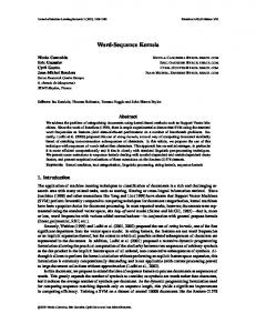
Table 4: The average time in milliseconds for each call to a specific kernel-function configured with specific parameter values. Tested data sets contain proteins with less than 200 residues (short), with more than 200, and less than 400 residues (medium) and with more than 400 residues (long). tween the predictions of two kernels. One kernel is chosen as a reference point. Whenever the other kernel produces the same positive predictions then these are considered true positives, if the second kernel produces a negative prediction where the first produces a positive, it is considered a false negative, and so on. The resulting pairwise correlations between the outputs of kernels can be found in Table 5. The highest correlating kernels are the Wildcard and Mismatch kernels, which seem to share more predictions than any of the other pairs of kernels. Although the parameters used by the Wildcard and Mismatch kernels are different, the correlation is to be expected due to the similar tactics they employ. The kernels whose prediction is least correlated are the Substitution and Local Alignment kernels. Additionally, they both correlated weakly with each of the other kernels, in particular with the Spectrum kernel. To investigate the qualititative nature of the feature spaces, we performed Kernel Principal Components Analysis (kernel-PCA) (Sch¨olkopf, Smola & M¨ uller 1999) on Problem set 1. In Figure 1, 10 inner membrane and 10 outer membrane proteins (arbitrarily selected from those subsets) are shown. Specifically, the samples are mapped onto the two dimensions with the largest eigenvalues in the Spectrum kernel k = 3 feature space and the Local Alignment kernel feature space, respectively. Kernel-PCA had access to all inner and outer membrane proteins. From Figure 1, we note that several samples are mapped differently to the feature space, e.g. Q51397 and Q55293 are quite distinct according to
Kernels Mismatch - Wildcard Spectrum - Mismatch LA - Profile LA Spectrum - Wildcard Mismatch - LA Wildcard - Subst Wildcard - LA Wildcard - Profile LA Mismatch - Profile LA Mismatch - Subst Spectrum - Subst Spectrum - LA Subst - LA Spectrum - Profile LA Subst - Profile LA
Problem 1 2 0.93 0.86 0.89 0.87 0.87 0.79 0.85 0.75 0.84 0.67 0.82 0.68 0.83 0.67 0.81 0.67 0.81 0.65 0.82 0.63 0.78 0.59 0.78 0.61 0.77 0.65 0.77 0.59 0.75 0.60
3 0.70 0.61 0.62 0.59 0.59 0.59 0.57 0.55 0.56 0.53 0.56 0.53 0.51 0.49 0.48
Average 0.83 0.79 0.76 0.73 0.70 0.69 0.69 0.68 0.67 0.66 0.64 0.64 0.64 0.62 0.61
Table 5: Correlation coefficients of predicted classifications from pairs of kernels. A correlation of 1 indicates that kernels enable the same predictions. A correlation of 0 indicates that there is chance agreement between predictions. the Spectrum kernel but similar according to the Local Alignment kernel. The outer membrane protein Q51922 is misclassified by both kernels but with different outcomes (“cytoplasm” for the Spectrum and “periplasm” for the Local Alignment kernel). The inner membrane protein Q52788 is confused for an outer membrane protein by both kernels (clearly occupying a space in the wrong feature space territory). 7
Conclusion
This paper takes a range of popular sequence kernels and compares their performance over a range of protein subcellular localization problems. Where the content of this study overlaps with previous comparative simulations we are in general agreement. Leslie and colleagues (Leslie et al. 2004) found that adding mismatches to spectrums improves the result on spectrums alone for protein remote homology classification. Furthermore, Saigo and colleagues (Saigo et al. 2004) found that the local alignment kernel outperforms the Mismatch kernel, again on the remote homology problem. Cheng and colleagues (Cheng, Saigo & Baldi 2006) also noted that the Local Alignment kernels outperformed both Mismatch and the Spectrum kernels on a protein disulphide bond detection problem set. Very recent developments indicate the potential of incorporating substitution profiles in the kernels (Rangwala & Karypis 2005, Kuang et al. 2005). We adapt the Local Alignment kernel to use such scores and also find that accuracy improves considerably. Although the overall performance of the kernels agrees with these results, the performance of the kernels was not consistent across the range of problems. These results demonstrate that when choosing kernels for specific problems, a range of kernels should be considered to ensure the most appropriate ker-
7 P03819
6
Q51397
5 4
P02941 3
O34245
2
P00550
O06873
0 −1
P00556
P00803
−2 Q934G3 −4
Q51240 Q48473
−2
Q55293
0
Q56989
2
4
4
P03819
3
P00550 P02941 O34245 P02933 Q51463 Q51397 O32522 Q55293 O52788
2 1 0 −1
O52788
Q54001
Q51485
Q51922
−3 −6
Q51463
O32522 P02933
1
O06873 P00803
P00556
Q54001
Q51922
−2
Q56989
Q51485
−3 Q934G3 −4 Q51240 Q48473
−5 −6 −15
−10
−5
0
5
10
Figure 1: Kernel Principal Component Analysis was performed on the Spectrum kernel k = 3 features space (above) and the Local Alignment feature space (below) using Problem set 1 (inner and outer membrane). The same samples are shown in both feature spaces. Each sample is labelled with its Swiss Prot identifier. Inner membrane proteins are plotted as red dots, outer membrane proteins are plotted as blue crosses. Samples that were misclassified in the reported simulations are underlined.
nel is chosen. The correlation between the predictions indicates that the Spectrum, Local Alignment and Substitution kernels are the most distinct methods for mapping sequences to a SVM feature space. However, the spectrum-based Mismatch kernel consistently outperforms the Spectrum kernel and can be easily substituted in its place. Suggesting that the ideal initial experiment should involve the Mismatch, Local Alignment and Substitution kernels to determine the kernel architecture to which the specific problem is suited. Comparing the kernels in terms of time consistency and efficiency, the Mismatch, Local Alignment and Substitution kernels perform worst. This illustrates that when it comes to choosing a kernel the trade-off between accuracy, correlation of errors and time efficiency can not be avoided with the reviewed range of kernels. Finally, in our benchmark on the sub-nuclear localization data set, none of the kernels performed satisfactorily. If we presume that this is not due to problems with the data, then we must conclude that the tested range of sequence kernels does not yet offer a complete toolkit for biological sequence classification. Acknowledgments This research was supported by the Australian Research Council Centre for Complex Systems and Centre for Bioinformatics. We thank Johnson Shih who implemented some of the kernels used in this study. References Cheng, J., Saigo, H. & Baldi, P. (2006), ‘Largescale prediction of disulphide bridges using kernel methods, two-dimensional recursive neural networks, and weighted graph matching’, Proteins: Structure, Function, and Bioinformatics 62(3), 617–629. Dellaire, G., Farrall, R. & Bickmore, W. (2003), ‘The nuclear protein database (npd): sub-nuclear localisation and functional annotation of the nuclear proteome’, Nucl. Acids Res. 31(1), 328– 330. Emanuelsson, O., Elofsson, A., von Heijne, G. & Cristobal, S. (2003), ‘In silico prediction of the peroxisomal proteome in fungi, plants and animals’, Journal of Molecular Biology 330(2), 443– 456. Gardy, J., Spencer, C., Wang, K., Ester, M., Tusnady, G., Simon, I., Hua, S., deFays, K., Lambert, C., Nakai, K. & Brinkman, F. (2003), ‘PSORT-B: improving protein subcellular localization prediction for gram-negative bacteria’, Nucl. Acids Res. 31(13), 3613–3617. Gordon, J. J., Towsey, M. W., Hogan, J. M., Mathews, S. A. & Timms, P. (2006), ‘Improved prediction of bacterial transcription start sites’, Bioinformatics 22(2), 142–148. Hawkins, J. & Bod´en, M. (2005), Predicting peroxisomal proteins, in ‘Proceedings of the IEEE Symposium on Computational Intelligence in Bioinformatics and Computational Biology’, IEEE, Piscataway, pp. 469–474. Hua, S. J. & Sun, Z. R. (2001a), ‘Support vector machine approach for protein subcellular localization prediction’, Bioinformatics 17(8), 721–728.
Hua, S. & Sun, Z. (2001b), ‘A novel method of protein secondary structure prediction with high segment overlap measure: support vector machine approach,’, Journal of Molecular Biology 308(2), 397–407. Jaakkola, T., Diekhans, M. & Haussler, D. (2000), ‘A discriminative framework for detecting remote protein homologies’, Journal of Computational Biology 7(1-2), 95–114. Kuang, R., Ie, E., Wang, K., Wang, K., Siddiqi, M., Freund, Y. & Leslie, C. (2005), ‘Profile-based string kernels for remote homology detection and motif extraction’, Journal of Bioinformatics and Computational Biology 3(3), 527–550. Lei, Z. & Dai, Y. (2005), ‘An SVM-based system for predicting protein subnuclear localizations’, BMC Bioinformatics 6(1), 291. Leslie, C., Eskin, E., Cohen, A., Weston, J. & Noble, W. (2004), ‘Mismatch string kernels for discriminative protein classification’, Bioinformatics 20(4), 467–476. Leslie, C., Eskin, E. & Grundy, W. S. (2002), The spectrum kernel: A string kernel for svm protein classification, in R. B. Altman, A. K. Dunker, L. Hunter, K. Lauerdale & T. E. Klein, eds, ‘Proceedings of the Pacific Symposium on Biocomputing’, World Scientific, pp. 564–575. Leslie, C. & Kuang, R. (2004), ‘Fast string kernels using inexact matching for protein sequences’, Journal of Machine Learning Research 5, 1435– 1455. Matthews, B. W. (1975), ‘Comparison of predicted and observed secondary structure of t4 phage lysozyme’, Biochim Biophys Acta 405, 442–451. Nakai, K. (2000), ‘Protein sorting signals and prediction of subcellular localization’, Advances in Protein Chemistry 54, 277–344. Neuberger, G., Maurer-Stroh, S., Eisenhaber, B., Hartig, A. & Eisenhaber, F. (2003), ‘Motif refinement of the peroxisomal targeting signal 1 and evaluation of taxon-specific differences’, Journal of Molecular Biology 328(3), 567–579. Park, K.-J. & Kanehisa, M. (2003), ‘Prediction of protein subcellular locations by support vector machines using compositions of amino acids and amino acid pairs’, Bioinformatics 19(13), 1656– 1663. Platt, J. (1999), Fast training of support vector machines using sequential minimal optimization, in B. Sch¨olkopf, C. J. C. Burgess & A. J. Smola, eds, ‘Advances in Kernel Methods–Suport Vector Learning’, MIT Press, Cambridge, MA, pp. 185–208. Rangwala, H. & Karypis, G. (2005), ‘Profile-based direct kernels for remote homology detection and fold recognition’, Bioinformatics 21(23), 4239– 4247. Saigo, H., Vert, J.-P., Ueda, N. & Akutsu, T. (2004), ‘Protein homology detection using string alignment kernels’, Bioinformatics 20(11), 1682– 1689. Sch¨olkopf, B. & Smola, A. (2002), Learning with kernels, MIT Press, Cambridge, MA.
Sch¨olkopf, B., Smola, A. & M¨ uller, K.-R. (1999), Kernel principal component analysis, in B. Sch¨ olkopf, C. J. C. Burges & A. J. Smola, eds, ‘Advances in Kernel Methods—Support Vector Learning’, MIT Press, Cambridge, MA, pp. 327–352. Wang, J., Sung, W.-K., Krishnan, A. & Li, K.B. (2005), ‘Protein subcellular localization prediction for gram-negative bacteria using amino acid subalphabets and a combination of multiple support vector machines’, BMC Bioinformatics 6(1), 174. White, S. H. & von Heijne, G. (2005), ‘Transmembrane helices before, during, and after insertion’, Current Opinion in Structural Biology 15(4), 378–386.