910
JOURNAL OF HYDROMETEOROLOGY—SPECIAL SECTION
VOLUME 6
Modeling Evapotranspiration during SMACEX: Comparing Two Approaches for Local- and Regional-Scale Prediction H. SU, M. F. MCCABE,
AND
E. F. WOOD
Department of Civil and Environmental Engineering, Princeton University, Princeton, New Jersey
Z. SU International Institute for Geo-Information Science and Earth Observation (ITC), Enschede, Netherlands
J. H. PRUEGER National Soil Tilth Research Laboratory, Ames, Iowa (Manuscript received 26 July 2004, in final form 5 April 2005) ABSTRACT The Surface Energy Balance System (SEBS) model was developed to estimate land surface fluxes using remotely sensed data and available meteorology. In this study, a dual assessment of SEBS is performed using two independent, high-quality datasets that are collected during the Soil Moisture–Atmosphere Coupling Experiment (SMACEX). The purpose of this comparison is twofold. First, using high-quality local-scale data, model-predicted surface fluxes can be evaluated against in situ observations to determine the accuracy limit at the field scale using SEBS. To accomplish this, SEBS is forced with meteorological data derived from towers distributed throughout the Walnut Creek catchment. Flux measurements from 10 eddy covariance systems positioned on these towers are used to evaluate SEBS over both corn and soybean surfaces. These data allow for an assessment of modeled fluxes during a period of rapid vegetation growth and varied hydrometeorology. Results indicate that SEBS can predict evapotranspiration with accuracies approaching 10%–15% of that of the in situ measurements, effectively capturing the temporal development of surface flux patterns for both corn and soybean, even when the evaporative fraction ranges between 0.50 and 0.90. Second, utilizing high-resolution remote sensing data and operational meteorology, a catchmentscale examination of model performance is undertaken. To extend the field-based assessment of SEBS, information derived from the Landsat Enhanced Thematic Mapper (ETM) and data from the North American Land Data Assimilation System (NLDAS) were combined to determine regional surface energy fluxes for a clear day during the field experiment. Results from this analysis indicate that prediction accuracy was strongly related to crop type, with corn predictions showing improved estimates compared to those of soybean. Although root-mean-square errors were affected by the limited number of samples and one poorly performing soybean site, differences between the mean values of observations and SEBS Landsat-based predictions at the tower sites were approximately 5%. Overall, results from this analysis indicate much potential toward routine prediction of surface heat fluxes using remote sensing data and operational meteorology.
1. Introduction Evaporation from the land surface and transpiration from plants combine to return available moisture at the surface layer back to the bulk atmosphere in a process Corresponding author address: Hongbo Su, Department of Civil and Environmental Engineering, Princeton University, Princeton, NJ 08544. E-mail:
[email protected]
© 2005 American Meteorological Society
referred to as evapotranspiration (ET). Because much of our understanding of the complex feedback mechanisms between the earth’s surface and the surrounding atmosphere is focused on quantifying this process, there is considerable interest in developing products that routinely predict this variable. Local- and regionalscale estimates of ET would offer insight into hydroecological processes, aid in improving irrigation efficiency, and provide a valuable tool for water resource management. Accurate estimation at large scales is re-
DECEMBER 2005
SU ET AL.
quired to improve our understanding of the global climate and its spatial and temporal variability (Miller et al. 1995). However, the prediction and validation of ET across all scales is often problematic. Uncertainties associated with pixel-scale heterogeneity are difficult to evaluate, and no robust in situ methods exist that reliably measure surface fluxes over large heterogeneous areas (Kustas and Norman 2000). Furthermore, where data do exist the representative area of surface flux measurements and the pixel scale of model-derived estimates are often quite different. Famiglietti and Wood (1994) suggest that at scales larger than 15 km, simulation error in land surface fluxes may arise as a result of the macroscale assumptions of areally averaged atmospheric forcing, vegetation parameters, and the methods by which these data and other flux observations are aggregated. There is a clear need for evapotranspiration products at scales commensurate with the underlying surface heterogeneity. Remote sensing offers much potential in bridging the gap between point- and larger-scale processes and identifying this “appropriate” model scale. However, one of the major shortcomings in advancing the application of techniques for flux prediction is the distinct lack of validation data that are available over diverse surface and atmospheric conditions against which techniques can be evaluated. The paucity of data extends (more critically) to surface forcing data, making it difficult to undertake model prediction, let alone validation. The Soil Moisture–Atmosphere Coupling Experiment (SMACEX) (Kustas et al. 2005) addresses this lack by providing a detailed and comprehensive observation of hydrological interactions over a watershed in central Iowa. Such campaigns allow a unique opportunity to assess model performance at a variety of temporal and spatial scales. The Surface Energy Balance System (SEBS) model was proposed by Su (2002) to estimate atmospheric turbulent fluxes and the evaporative fraction (the ratio of latent heat flux to the available energy) using satellite data and ancillary surface and meteorological information. SEBS is physically based and has the potential to be used across local, regional, and continental scales with remotely sensed data and standard meteorological observations. However, when estimating ET at increasing spatial scales (greater than 1 km), uncertainties resulting from the process model and its parameters and those incurred because of heterogeneities at the land surface are often coupled. As such, it is beneficial for a model to be robustly assessed at local scales where accurate forcing and validation data are available, before attempting larger-scale applications. Recently, SEBS
911
has been used in a preliminary study to estimate regional evapotranspiration using the Moderate Resolution Imaging Spectroradiometer (MODIS) data (Wood et al. 2003), and also to predict the sensible heat flux using Along Track Scanning Radiometer (ATSR) measurements (Jia et al. 2003). However, further validation of the approach is required to both assess the model of varied climatic conditions and aid in developing an accurate estimation of evapotranspiration at a variety of satellite resolutions. The purpose of this paper is to determine the ability of SEBS to predict evapotranspiration at both local and regional scales, over the varied hydrometeorological conditions that are evident during SMACEX. The analysis represents an important step toward the use of SEBS in routinely predicting terrestrial evapotranspiration from MODIS-based satellite data as part of the National Aeronautics Space Administration’s (NASA’s) Earth Observing System. Section 2 presents a brief description of the model, and section 3 introduces the two distinct forcing datasets used to independently assess the model at both local and regional scales. Although modeling at the local scale circumvents the impediment of subpixel heterogeneity, the results presented in section 4a offer some insight into achievable accuracies and model performance when undertaking analysis at scales where such issues are unavoidable. To explore this further, SEBS results using remote sensing and operational forcing data are presented in section 4b. Landsat Enhanced Thematic Mapper (ETM) and forcing data derived from the North American Land Data Assimilation System (NLDAS) were used to estimate regional surface energy fluxes across the SMACEX domain, independent of in situ observations. For both local- and regional-scale studies, ET estimates are compared with independently measured tower-based flux observations. Section 5 discusses the variety of issues associated with flux prediction at both the local and regional scale and identifies the potential for determining routine estimates of evapotranspiration from remote sensing.
2. Model description The SEBS model (Su 2002) was developed to estimate surface energy fluxes and the evaporative fraction using remotely sensed data in combination with meteorological information at scales that were dependent on the forcing data. SEBS consists of several separate modules to estimate the net radiation and soil heat flux, and to partition the available energy into sensible and latent heat fluxes, of which a brief introduction is presented below.
912
JOURNAL OF HYDROMETEOROLOGY—SPECIAL SECTION
The surface energy balance equation is commonly written as Rn ⫽ G0 ⫹ H ⫹ E,
共1兲
where Rn is the net radiation, G0 is the soil heat flux, H is the sensible heat flux, and E is the latent heat flux. In a satellite remote sensing application with SEBS, net radiation is estimated based on radiative energy balance: Rn ⫽ 共1 ⫺ ␣兲Rswd ⫹ Rlwd ⫺ T s4,
共2兲
where ␣ is the broadband albedo in the visible and near-infrared band, is the broadband emissivity in the thermal infrared band, Rswd is the incident solar radiation, Rlwd is the downward longwave radiation, Ts is the surface temperature, and is the Stephan–Boltzman constant. The other component comprising the available energy is the soil heat flux. In the absence of observed soil heat flux measurements, as in satellite applications or at large regional scales, empirical formulations of the soil heat flux based on net radiation and the vegetation fraction are used to estimate the total soil heat flux for the area. If the soil heat flux ratio is defined as ⌫ ⫽ G0ⲐRn,
共3兲
then the soil heat flux can be parameterized following Monteith (1973) and Kustas and Daughtry (1990): G0 ⫽ Rn关⌫ f ⫹ ⌫s共1 ⫺ f兲兴,
共4兲
where ⌫ and ⌫s are the soil heat flux ratios for full vegetation canopy and for bare soil respectively, and f is the vegetation fraction. The remaining variable that SEBS independently estimates is the sensible heat flux H, which is solved using a combination of the three equations below: u⫽
0 ⫺ a ⫽
冋 冉 冊 冉 冊 冉 冊册 冋 冉 冊 冉 冊 冉 冊册
u z ⫺ d0 z ⫺ d0 z0m * ln ⫺ ⌿m ⫹ ⌿m k z0m L L
H z ⫺ d0 z ⫺ d0 z0h ln ⫺ ⌿h ⫹ ⌿h ku Cp z0h L L * 3
L⫽⫺
Cpu * , kgH
共5兲
where u is the wind speed, u is the friction velocity, * is the air density, Cp is the specific heat of air at constant pressure, k is the von Kármán constant, d0 is the zero-plane displacement, z is the height above the surface, z0m and z0h are the roughness height for momentum and heat transfer, respectively (Su et al. 2001), 0
VOLUME 6
and a are the potential temperatures at surface and at height z, respectively, ⌿h and ⌿m are the stability correction functions (Brutsaert 1999) for sensible heat and momentum transfer respectively, L is the Obukhov length, g is the acceleration resulting from gravity, and is the virtual temperature near the surface. The three unknowns in the above equations are L, H, and u . * In SEBS, the model output of sensible and latent heat fluxes is also constrained by considering dry-limit and wet-limit conditions, which give the upper and lower boundary of sensible heat flux estimation. Further details on the particular techniques used to separate the sensible and latent heat flux from the available energy can be found in Su (2002).
3. Data description and methodology SMACEX was conducted in Iowa from 19 June through 9 July in 2002. The primary goal of the field campaign was to use a combination of direct measurements, remote sensing, and modeling approaches to understand how horizontal heterogeneities in vegetation cover, soil moisture, and other land surface variables influence the exchange of moisture and heat with the atmosphere (USDA ARS Hydrology and Remote Sensing Lab 2002). Walnut Creek, a small watershed in central Iowa, was the focus of investigations during SMACEX. Nearly 95% of the region and watershed is used for row crop agriculture, with corn and soybean representing approximately 80% thereof in relatively equal proportions. Further details and a description of the experiment can be found in Kustas et al. (2005). Two scenarios have been designed to assess the SEBS model here. One is to use all available in situ measurements in SMACEX as forcing data, while the other is to use operational meteorological and satellite data. The model outputs of surface energy fluxes in both situations are then compared with those from the tower measurements. The data requirements and sources, as well as the processing of the data, are described in the following sections.
a. Local-scale forcing and model data The in situ measurements used by SEBS are listed in Table 1 (referred to as dataset I). In addition to towerbased flux measurements and meteorological data, other observations, including detailed vegetation parameters and surface meteorological data, were also collected during the campaign (Kustas et al. 2005). In this case, the observations of solar insolation, downward longwave radiation, and soil heat flux were used directly in the SEBS model as input data to compute
DECEMBER 2005
913
SU ET AL.
TABLE 1. SEBS model data requirements (dataset I). All inputs are determined from available in situ measurements. The observations in italic are used for validation purposes. Data type
Variables
Unit
Surface meteorological data
Air temperature Pressure Wind Vapor pressure Incident shortwave radiation Outgoing shortwave radiation Incident longwave radiation Outgoing longwave radiation Net radiation Ground heat flux Sensible heat flux Latent heat flux Evaporative fraction Composite radiometric temperature (soil ⫹ vegetation) Vegetation height Vegetation fraction Leaf area index Vegetation type (corn or soybean)
°C kPa m s⫺1 kPa W m⫺2 W m⫺2 W m⫺2 W m⫺2 W m⫺2 W m⫺2 W m⫺2 W m⫺2 — °C m — — —
Radiative energy flux
Surface heat flux
Surface temperature Vegetation parameters
the available energy. The meteorological and heat flux data were measured every 10 min. In this study, the data were resampled to 30 min. The three categories of forcing data will be described below.
1) METEOROLOGICAL
DATA AND SURFACE
TEMPERATURE
Standard meteorological forcing data, including wind velocity, vapor pressure, air temperature, and atmospheric pressure, were used to run the SEBS model. A key variable in application of the SEBS model is the land surface temperature. During SMACEX, the tower-based composite (including soil and vegetation) radiometric surface temperature was measured by Apogee infrared thermometers (model IRTS-P) (Jackson and Cosh 2003). Bugbee et al. (1999) suggest a method to correct the brightness temperature for differential heating of the sensor. According to instrument specifications, the accuracy of the brightness temperature (TB) is within 0.4°C after the correction. Simulations conducted as part of this analysis indicate that the error induced in surface temperature estimates by the substitution of the narrowband brightness temperature (6–14 m) for that of the broadband (5–50 m) introduces minimal error with respect to the standard accuracy of the Apogee sensor. A constant emissivity of 0.97 is assigned to all tower sites to estimate the surface temperature, in combination with the measurements of downward longwave radiation and corrected brightness temperature from the infrared thermometer measurements.
2) VEGETATION
PARAMETERS
In SEBS, the leaf area index (LAI) and vegetation fraction are used to estimate (i) the roughness height for heat and momentum transfer, (ii) the mixed emissivity when remote sensing data are employed (to derive the surface temperature), and (iii) the ground heat flux over a region, if unavailable from measurements. Correctly representing the variation of the vegetation over the course of the field campaign is crucial to obtaining an accurate reproduction of the surface fluxes. LAI, vegetation fraction, and vegetation height were measured on four separate occasions at each of the tower sites on 18 and 28 June and 2 and 5 July, respectively. To be compatible with the temporal resolution of the observation data used in the model assessment, the vegetation parameters require temporal expansion from 20 June through 9 July. Both a linear and nonlinear interpolation techniques are employed for the two types of vegetation parameters. Based on the observed temporal patterns of LAI and vegetation height during the growing seasons for corn and soybean, a simple linear interpolation is used to generate daily LAI and vegetation height from the four days of observations. However, it has been reported that the relationship between the vegetation fraction and LAI is often nonlinear (Nilson 1971; Chen and Cihlar 1995), potentially causing inconsistency between the vegetation parameters if a linear interpolation is used. Thus, a nonlinear relationship between LAI and the vegetation fraction is formulated to make full use of the vegetation measurements and maintain consistency between observations.
914
JOURNAL OF HYDROMETEOROLOGY—SPECIAL SECTION
Following Chen and Cihlar (1995), the vegetation fraction can be formulated with LAI using
冋
f 共兲 ⫽ 1 ⫺ exp
册
⫺共兲 · LAI , cos共兲
共6兲
where f() is the directional vegetation fraction, is the zenith view angle, and () is a combination of the mean projection of the unit leaf area on the plane perpendicular to the beam direction and the clumping factor, which represents the spatial distribution pattern of the foliage. In this study, because no multiangle vegetation fraction was available, we are only interested in the vegetation fraction when viewed at nadir. Equation (6) is used to fit a nonlinear relationship between vegetation fraction and LAI for corn and soybean, respectively, based on in situ observations. The formulation is subsequently used to estimate the vegetation fraction at a daily scale at each site using the interpolated LAI.
b. Regional-scale forcing and remote sensing data On a routine basis, in situ measurements are not generally available for model forcing. As a result, data from satellite and operational meteorology offer the best surrogate for local measurements. Table 2 outlines the data requirements and sources of the meteorological and satellite products employed in the regionalscale analysis (referred to as dataset II). The original data represent a variety of resolutions according to the different data sources, and interpolation has been employed, where necessary, to standardize the measurements.
1) NLDAS
DATA
Meteorological forcing data, such as wind velocity, humidity, pressure, air temperature, and downward longwave radiation, were extracted from the NLDAS (Cosgrove et al. 2003). NLDAS has a spatial resolution of 0.125° and provides information at an hourly time step. It has been extensively validated and is indicated TABLE 2. SEBS model data requirements (dataset II). All inputs are based on operational meteorological and satellite data. Data source NLDAS
Landsat-7 ETM⫹ MODIS GOES
Variables
Unit
Resolution
Air temperature Pressure Wind Specific humidity Downward longwave radiation Brightness temperature NDVI Land cover Albedo Surface insolation
°C Pa m s⫺1 — W m⫺2
1/8°
K — — — W m⫺2
60 m 30 m 30 m 1 km 20 km
VOLUME 6
to be an excellent dataset for land surface modeling (Luo et al. 2003). To match with the Landsat temperature data, the NLDAS data at 1000 and 1100 central standard time (CST) were interpolated linearly to obtain the meteorological data at 1040 CST.
2) LANDSAT ETM
DATA
To capture the heterogeneity of the land surface over the SMACEX domain, high-resolution satellite data are required. Landsat-7 ETM overpasses (approximately 1040 CST) were collected during the field campaign on 1 and 8 July. Only data from 1 July are used here because of striping in the 8 July overpass. The Landsat ETM data provide high-resolution information on the land surface brightness temperature (Li et al. 2004), land cover classification, and the Normalized Difference Vegetation Index (NDVI). However, there is a spatial mismatch between the 60-m surface temperature (derived from the thermal band) and the 30-m land and vegetation information. To maintain consistency, the surface temperature data were interpolated to 30 m using a nearest-neighbor technique. While averaging the surface temperature is not strictly correct (because of the nonlinearity in the Planck function), it is not expected to introduce significant error at this scale. Using the Landsat vegetation data requires some transformation relating LAI and vegetation fraction to NDVI. Xavier and Vettorazzi (2004) present an experimentally determined relationship of the following form: NDVI ⫽ 0.6868共LAI0.1810兲.
共7兲
2
An r of 0.72 and an rms error of 0.06 were determined for their experiment, which included corn crops as one of the samples. The vegetation fraction ( f) can be estimated from NDVI using the formulation of Baret et al. (1995): f ⫽ 1 ⫺
冉
NDVI ⫺ NDVI⬁ NDVIs ⫺ NDVI⬁
冊
k
,
共8兲
where NDVIs represents the value for bare soil (0.2013), NDVI⬁ is the value for a full canopy (0.8986), and k is 0.6175, all of which were experimentally determined. A recent study on the emissivity values for a heterogeneous surface (Chen et al. 2004) showed that a linear relationship between the soil and vegetation emissivity is sufficient to compute the effective emissivity and, subsequently, the surface temperature. The effective emissivity can be calculated linearly using the following equation (Chen et al. 2004): e ⫽ f ⫹ s 共1 ⫺ f兲,
共9兲
where e is the effective emissivity, f denotes the vegetation fraction, and and e are the emissivities for vegetation and soil, respectively. Vegetated surface are
DECEMBER 2005
given a value of 0.985 while the bare soil has an emissivity of 0.978 (Sobrino et al. 2001; Li et al. 2004). One thing to note is that the Landsat emissivity may be different from an infrared thermometer when the target is not a graybody, because the bandwidth (10.4–12.5 m) is generally narrower than that of the infrared thermometer (8–14 m).
3) ADDITIONAL
915
SU ET AL.
SATELLITE DATA
The Geostationary Operational Environmental Satellite (GOES) offers the opportunity to determine surface insolation (net shortwave radiation) using the approach of Diak et al. (1996) and Jacobs et al. (2002). Data for the study period was provided by the University of Wisconsin—Madison (M. C. Anderson 2004, personal communication) at hourly time steps and a spatial resolution of 20 km. To determine the outgoing shortwave radiation, knowledge of the albedo is required. Broadband albedo is determined from the MODIS data (Schaaf et al. 2002). A true surface albedo product is not currently available, so an average of the provided black-sky and white-sky albedo were used as an estimate for this variable. While the true surface albedo is also a function of atmospheric optical depth, it is not expected that the exclusion of this will unduly influence results.
c. Flux validation data The eddy covariance technique estimates sensible and latent heat fluxes by measuring fluctuations in heat and moisture covariances with respect to vertical velocity (Kanemasu et al. 1992). Independent measurements of the latent and sensible heat fluxes during SMACEX were using a 3D sonic anemometer and a LI-COR 7500 water vapor/CO2 sensor (Kustas et al. 2005). These individual measurements allow for an assessment of energy balance closure to be made, given that the net radiation and soil heat flux are also observed. There are 14 tower sites distributed throughout the SMACEX domain, 12 of which have flux measurements. Of these, two sites (WC14 and WC25) are listed in the quality control documentation as requiring despiking to remove spurious observations. These are not used in assessing flux comparisons. For the analysis undertaken here, 10 flux tower sites evenly distributed between corn and soybean fields are used to assess the local- and regional-scale modeling.
It is well recognized, if not well understood, that field measurements of heat fluxes using the eddy covariance technique often fail to show closure of the surface energy budget (Brotzge and Crawford 2003; Massman and Lee 2002). During SMACEX, the average closure rate during the daytime, defined as the sum of the heat fluxes (LE ⫹ H ) over the available energy (Rn ⫺ G), was 0.71 for a typical soybean site. A corresponding corn site indicates an average closure rate of 0.84, highlighting the necessity to correct these validation measurements. To satisfy the nonclosure problem that is evident in the SMACEX data, a Bowen ratio closure method is adopted to correct the sensible and latent heat flux measurements. Essentially, this approach assumes that the Bowen ratio is correctly measured by the eddy covariance system, allowing individual fluxes to be adjusted (see Twine et al. 2000). Further information on the correction of the eddy covariance data using such closure techniques is provided in Prueger et al. (2005).
4. Results a. Local-scale evaluation SEBS was run at a temporal resolution of 30 min during the daytime (from 1000 to 1600 CST) over the 20 days of SMACEX measurements at each of the 10 flux tower sites. In this section, predicted evapotranspiration from the SEBS model is compared with those derived from observations, allowing the accuracy of the model prediction to be assessed.
1) TEMPORAL
PATTERN OF SURFACE FLUXES AT
TOWER SITES
To determine the ability of the SEBS model to accurately reproduce the land surface fluxes, a time series comparison between modeled sensible and latent heat fluxes and those from corrected eddy covariance measurements was undertaken. Three sites were selected to illustrate the temporal comparison and characterize the response of the different vegetation types being modeled during the daytime period from day of year (DOY) 171 through 190. A corn site (WC06), a soybean site (WC03), and a poorly performing soybean site (WC13) are chosen to illustrate the dynamics of the surface flux response and are show in Fig. 1. Site WC13 →
FIG. 1. Time series of latent heat (嘷) and sensible heat (䉭) fluxes for observations (closed) and model predictions (open) at selected (a) corn and (b), (c) soybean sites. Data are shown only for the daytime period (1000–1600 CST), with major tick marks indicating the first morning measurement. Gaps in the time series are caused by either the absence of flux measurements or missing ancillary data.
916
JOURNAL OF HYDROMETEOROLOGY—SPECIAL SECTION
VOLUME 6
DECEMBER 2005
917
SU ET AL.
FIG. 2. SEBS-predicted latent heat flux vs eddy covariance based observations for (a) corn sites WC06, WC151, WC152, WC24, and WC33; (b) soybean sites SC03, WC162, and WC23; (c) soybean sites WC13 and WC161; and (d) soybean sites WC13 and WC161 with corrected emissivity.
is selected to be representative of the two soybean sites (WC13 and WC161) where the model tends to overestimate the latent heat flux over the first 10 days. Figure 1 reveals that observations from both the soybean (WC03) and corn (WC06) sites agree very well with model predictions of ET from SEBS. Excluding the first day of measurements, consistent agreement throughout the period is observed over the daily cycle, with a steady level of evapotranspiration that is evident through DOY 171–185. Evaporation from the corn crop is approximately 100–150 W m⫺2 greater than the soybean crop and also exhibits a stronger diurnal trend during the daytime. The effect of precipitation on DOY 186–188 triggers a steady rise in the evapotranspiration rate, with values as high as 555 and 582.3 W m⫺2 recorded at soybean and corn sites, respectively. These
values represent well over 90% of the available energy at each of the two sites. Generally, a much closer agreement for all sites is apparent during the last 10 days when the evapotranspiration is slightly higher.
2) SPATIAL REPRESENTATION ACROSS SMACEX
OF SURFACE FLUXES
Scatterplots of ET predictions from SEBS against observed latent heat flux at the SMACEX tower sites are presented in Fig. 2. These plots allow for an alternative assessment of the individual time series development (Fig. 1), offering an examination of model performance across both the spatial and temporal domain. An overview of the statistics for each of the graphs is presented in Table 3. For the corn sites (Fig. 2a), an even distribution about the unity gradient illustrates the good fit
918
JOURNAL OF HYDROMETEOROLOGY—SPECIAL SECTION
VOLUME 6
TABLE 3. Statistical variation of the evapotranspiration estimates from SEBS based on dataset I during the SMACEX campaign. Values are given for the mean, bias, r2, rmse, mean absolute error (MAE), rrmse, relative bias (RB), and the relative MAE (MAE), with all flux units in W m⫺2.
Meanobs Bias r2 RBias Rmse rrmse MAE RMAE
Corn sites
Soybean sites (WC03, WC162, WC23)
Soybean sites (WC13, WC161)
Emissivity-corrected soybean (WC13, WC161)
350.44 ⫺6.68 0.89 1.91% 46.68 13.32% 34.08 9.73%
288.03 17.37 0.84 6.03% 40.39 14.02% 30.86 10.72%
237.97 56.78 0.82 23.86% 71.17 29.91% 61.88 25.99%
238.44 16.09 0.80 6.76% 48.00 20.15% 38.10 15.99%
of predictions to the measured fluxes, with an r 2 of 0.89 and an rms of 46.68 W m⫺2. The relative root-meansquare error (rrmse), defined as the rmse divided by the mean of the observations (Conte et al. 1986), is chosen as one of the criteria to evaluate the model accuracy. For corn, the relative rms is 13.32%, comparable to the error of in situ measurement techniques. At two soybean sites (WC13 and WC161), the SEBS model overestimated the latent heat flux during the first 10 days (see Fig. 1c), with a clearly distinguishable bias evident. Results for the soybean sites are separated to more clearly assess the reproduction of fluxes over this vegetation unit. The three well-performing responses (Fig. 2b) illustrate a good fit, with an r 2 of 0.84 and an rms of 40.39 W m⫺2, slightly lower than the corn crop. On the other hand, flux predictions at the two discriminated sites (Fig. 2c) indicate an offset in predictions, with analysis discerning a positive bias of over 56 W m⫺2, although results remain highly correlated with an r 2 of 0.81. The bias that is evident in both of the soybean sites (17.37 and 56.78 W m⫺2) is considerably greater than that for corn at ⫺6.68 W m⫺2. There are a number of possible explanations for the relatively poor representation of the two soybean sites. While observations of the downward longwave radiation from site WC151 are used for WC13 and WC161, this is not expected to be a significant source of error, because of its relatively low spatial variability. A shift in the closure rate for the eddy covariance measurements was observed over the course of the campaign. During the first 10 days, the average closure rate over the daytime is 0.91, while in the last 10 days the average closure rate was 0.81. It follows, then, that the correction coefficient (the inverse of the closure rate) is lower in the first 10 days than in the last 10 days. Brotzge and Crawford (2003) identified that the energy balance closure varies with season and time of day, introducing additional uncertainties into results. Another plausible explanation is error in the land surface parameters, such
as in the vegetation information, emissivity, or surface temperature. Closer examination of these two sites indicates that the vegetation fractions were the lowest for all sites, with the average vegetation fraction in the first 10 days for WC13 equaling 0.25, while for WC161 it was 0.35. Such a result would indicate that the emissivity might be overestimated if a constant value of emissivity is assigned to the two soybean sites during the observation period. To assess this, a new effective emissivity is calculated by assigning a vegetation emissivity of 0.98 and a soil emissivity of 0.94, from Chen et al. (2004), for a broadband approach. Using Eq. (9) to calculate the effective emissivity in the field of view of the infrared thermometer, the surface temperature can be solved. The model outputs for the two soybean sites using the corrected emissivity are presented in Fig. 2d. A significant reduction in bias (16.09 W m⫺2) and rms error (45.5 W m⫺2) was obtained at the expense of a slight reduction in r2 (0.798). The difference between model predictions and observation has been reduced significantly through the effective emissivity correction, although the deviation for these two soybean sites is still larger than all other sites. The statistical analyses of the corrected model output for these sites are listed in the last column of Table 3. Apart from emissivity affects, scale disparity between point-scale measurements of the surface temperature, incorrect characterization of vegetation properties, or errors in the eddy covariance measurements could all influence the equivalence of flux results. Scale issues are particularly pervasive in such comparisons and inevitably complicate the effective assessment of model output, given that they are not easily quantified. Current investigations focusing on achievable accuracies at a variety of resolutions from the point though to regional scales, should offer some insight into these processes. The relative rms and relative mean absolute error of the modeled ET estimates for the five corn sites are 13.32% and 9.73%. For the three soybean sites,
DECEMBER 2005
919
SU ET AL.
FIG. 3. Regional-scale latent heat flux estimates from SEBS using Landsat-, MODIS-, GOES-, and NLDAS-derived data. The Walnut Creek catchment and the distribution of flux towers throughout the region are also presented. Darker shades represent the soybean field sites, with lighter shades being the corn. Flux towers are distinguished as either being cornfields (triangles) or soybean fields (circles).
these values are 14.02% and 10.72%, respectively, indicating that there is no significant difference between the relative accuracies of the SEBS ET estimation over either corn or soybean crops.
b. Regional-scale evaluation SEBS Landsat-based estimates of the surface heat fluxes for 1 July (1040 CST time) were calculated for the SMACEX region using operational meteorological and ancillary remote sensing data. Figure 3 shows the latent heat flux estimation and the location of the flux tower sites over the catchment, illustrating the clear delineation between soybean and corn sites. To compare predictions with tower-based flux measurements, a 3 ⫻ 3 pixel box (90 m ⫻ 90 m) centered over each tower was extracted and the mean latent flux prediction was calculated. The results for SEBS Landsat-based surface fluxes over both corn and soybean sites are presented in Table 4, identifying the mean, bias, and rmse. Evapotranspiration estimates were assessed against the eight flux tower sites available for comparison on this day. Table 4 indicates that the mean latent heat flux at corn sites is larger than at soybean sites, consistent with in situ results. The latent heat flux difference between corn and soybean sites is approximately 120 W m⫺2 from in situ observations and 92.0 W m⫺2 from SEBS
Landsat predictions. Individual rms errors for corn and soybean were calculated as 28.7 and 84.9 W m⫺2, respectively, while the combined error for all sites was 60.6 W m⫺2. Clearly the results for soybean are not consistent with those for corn, with a large disparity in the retrieval accuracies. Closer analysis of the three tower sites available for comparison reveals the influence of site WC161, identified previously as one of the poorly performing sites in the local-scale analysis. The differences between observation and model predictions at TABLE 4. Statistics of the surface energy flux comparison between SEBS Landsat predictions based on dataset II and the in situ tower measurements at 1040 CST 1 Jul 2002.
LE
H
Crop type of the sites
Corn
Soybean
Corn and soybean
No. of available sites Mean from OBS (W m⫺2) Mean from SEBS (W m⫺2) Bias (W m⫺2) Rmse (W m⫺2) No. of available sites Mean from OBS (W m⫺2) Mean from SEBS (W m⫺2) Bias (W m⫺2) Rmse (W m⫺2)
5 459.3 450.5 ⫺8.8 28.7 5 95.5 81.2 ⫺14.2 23.8
3 339.9 358.5 18.6 84.9 3 172.3 111.2 ⫺61.0 86.3
8 414.6 416.0 1.4 60.6 8 124.3 92.5 ⫺31.8 60.0
920
JOURNAL OF HYDROMETEOROLOGY—SPECIAL SECTION
FIG. 4. Comparison of the energy fluxes from SEBS Landsatbased estimates and in situ observations at tower sites. Circles represent corn sites, while triangles signify soybean fields. Solid symbols identify the sensible heat flux and open symbols the latent heat flux. The range of results present in tower observations is shown in the x error bars and the standard deviation of satellitebased estimates across the region in y error bars. The regional average heat flux (across the domain in Fig. 3) is shown at the intersection of these lines.
this site are approximately 130 W m⫺2, explaining, to a large degree, the high rms error for the soybean sites collectively. WC161 is also located adjacent to a cornfield. As a result, averaging a 3 ⫻ 3 area around this site will likely sample from within the higher evaporating corn site. Comparing the mean values of the latent heat fluxes determined from Landsat and those from the tower observations indicate improved agreement. For corn, the difference between the means of the SEBS Landsat-based 3 ⫻ 3 estimates and the five corresponding tower values is less than 2%, while for the three soybean sites it is approximately 5%. Although the results here indicate much promise, the low number of validation points makes broad conclusions on the accuracy of such retrievals at the local scale difficult. However, one of the advantages of using remote sensing data is that the spatial variability can be studied explicitly and compared to point-scale measurements. Figure 4 presents the results of the mean latent and sensible heat fluxes calculated for corn and soybean sites across the domain presented in Fig. 3, as well as the 3 ⫻ 3 pixel averages (see Table 4) compared with tower-based observations. To estimate the degree of spatial variability throughout the region, the range in flux tower measurements and the standard deviation of the SEBS Landsat-estimated fluxes across the region are also included. The range is represented by the x error bars, while the standard deviation is shown in the
VOLUME 6
y error bars, with triangles representing the soybean and circles the corn sites. Generally, Fig. 4 indicates that retrievals for corn seem to agree more closely with observations than those for soybean, for both latent and sensible heat fluxes. Interestingly, soybean has an approximately 60% smaller standard deviation relative to corn in both surface fluxes, indicating greater flux consistency within soybean fields. The range of latent heat flux observations is approximately 65 W m⫺2 for corn and 100 W m⫺2 for soybean, although the latter result is again influenced by site WC161. For sensible heat fluxes, the ranges are more equivalent, being 64 and 80 W m⫺2 for corn and soybean, respectively. Overall, the observations from the tower sites seem to be representative of the regional average determined from the SEBS Landsat results, particularly so for corn. The variability of soybean results evident in Fig. 4 highlights the difficulty in characterizing flux measurements for large areas, even where good validation data are available for this purpose.
5. Discussion While the eddy covariance approach is perhaps the most direct means of measuring the water vapor flux, the instrumentation required to do this is quite sophisticated. As observed within the SMACEX observation data, the instruments are also prone to error, particularly in the regular inability to close the energy balance. Sensor misalignment can also result in the interference in measurements and incorrect sampling of downwind aerodynamic properties, which is integral to the accurate estimation of the flux characteristics of the upwind area (see Laubach and Teichmann 1999; Lee and Black 1994). To assess whether the performance of modeled latent heat fluxes provide adequate representations of surface behavior, an estimate of the uncertainties in measuring the surface fluxes in the field is required. A number of studies have assessed accuracies from standard in situ techniques such as the Bowen ratio and eddy covariance approaches (Fritschen et al. 1992; Nie et al. 1992; Lloyd et al. 1997). From these and other analyses, eddy covariance observations taken under ideal site conditions are likely to achieve accuracies in the of range 5%–15%, but can potentially be much worse. Given these findings, the accuracies in the evapotranspiration as determined for the SEBS model at both the local and regional scales are comparable with those achievable from in situ measurements. While the intersite variability over the corn sites was consistent between measurements (see Fig. 4), disparities between soybean observations and measurements
DECEMBER 2005
921
SU ET AL.
were observed between site locations, affecting the overall accuracy of model predictions. A number of possible explanations, including incorrect parameterizations, emissivity corrections, and scale disparities were offered. Another possibility is that different correction methods, other than the Bowen ratio closure approach used here, may be required for eddy covariance observations in soybean fields. The results presented here indicate that there are many factors that affect the modeling of surface heat fluxes, not all of which can be adequately accounted for. To improve the accuracy of model prediction, quality control of forcing and validation data and the description of land surface parameterizations are critical. This becomes even more crucial at coarse scales, but is made difficult by a lack of understanding of the scaling behavior of land surface parameters and fluxes. Observed available energy is used in this study when SEBS is applied at the local scale. At regional scales, however, the net radiation and soil heat fluxes are not routinely available, requiring that the regional available energy, along with other land surface parameters, be estimated with an accuracy that is adequate to ensure correct surface flux partitioning. Such issues continue to complicate the accurate retrieval of evapotranspiration, particularly over surfaces where no validation data exist. Using operational meteorological forcing data, such as is available from the NLDAS, offers an ideal pathway toward achieving robust predictions of regional-scale surface fluxes from remote sensing. While the analysis here offers a retrospective determination of fluxes, the potential exists to employ such data at near– real times, allowing for improved characterization of fluxes at time scales that are suitable for use in weather prediction, water resource management, or agricultural applications. Through the incorporation of data derived from three satellite platforms (Landsat, GOES, and MODIS) and obtaining meteorological forcings from a coarse-scale operational dataset, flux predictions displaying considerable agreement with in situ observations could be achieved. This represents a significant step toward characterizing surface behavior where in situ data are not routinely available.
6. Conclusions In this study, the SEBS model has been evaluated at local and regional scales using both in situ data and operational meteorology. Results indicate that surface flux predictions from SEBS perform very well when assessed against in situ flux measurements derived from eddy covariance approaches at both scales. For corn and soybean crops, SEBS does not exhibit significant
difference in the relative accuracy of the evapotranspiration estimate, although absolute values are clearly different and affected by individual flux observations. Results from the local-scale analysis determined a relative root-mean-square error and root mean absolute error of 13.32% and 9.73%, respectively, for the five corn sites. For the three soybean sites (excluding WC13 and WC161), these errors are 14.02% and 10.72%, respectively. Given the capabilities and limitations of both the eddy covariance and Bowen ratio approaches, accuracies in ET predictions from SEBS were equivalent to in situ measurement accuracies. Time series comparison of the model output and observations also show that SEBS correctly interprets hydrological variability and is capable of accurately representing the temporal development of evapotranspiration at the local scale. The SEBS model shows much promise in applications at regional scales and larger using satellite and ancillary forcing data at corresponding scales. Land surface parameters from MODIS land product data, radiation information from GOES, and meteorological data from the NLDAS form a sufficient database with which to run the SEBS model at such scales. Current investigations are focused on applying the SEBS model across a number of resolutions to study issues of scaling in evapotranspiration at the land surface. Acknowledgments. The authors thank the anonymous reviewers for their useful comments and suggestions to improve the manuscript. Particular thanks are due to Dr. Fuqin Li and Dr. Tom Jackson of the USDA for their provision of Landsat data used in the regional analysis, and also Dr. Martha Anderson of the University of Wisconsin—Madison for the supply of GOESbased surface insolation data. The contributions of the numerous participants and organizers of both the SMEX02 and SMACEX campaigns are greatly appreciated. Research was supported by funding from NASA Grant NNG04GQ32G: A Terrestrial Evaporation Product Using MODIS Data. REFERENCES Baret, F., J. G. P. W. Clevers, and M. D. Steven, 1995: The robustness of canopy gap fraction estimates from red and nearinfrared reflectances—A comparison of approaches. Remote Sens. Environ., 54, 141–151. Brotzge, J. A., and K. C. Crawford, 2003: Examination of the surface energy budget: A comparison of eddy correlation and Bowen ratio measurement systems. J. Hydrometeor., 4, 160– 178. Brutsaert, W., 1999: Aspects of bulk atmospheric boundary layer similarity under free-convective conditions. Rev. Geophys., 37, 439–451.
922
JOURNAL OF HYDROMETEOROLOGY—SPECIAL SECTION
Bugbee, B., M. Droter, O. Monje, and B. Tanner, 1999: Evaluation and modification of commercial infrared-red transducers for leaf temperature measurement. Adv. Space Res., 22, 1425–1434. Chen, J. M., and J. Cihlar, 1995: Quantifying the effect of canopy architecture on optical measurements of leaf area index using two gap size methods. IEEE Trans. Geosci. Remote Sens., 33, 777–787. Chen, L. F., Z.-L. Li, Q. H. Liu, S. Chen, Y. Tang, and B. Zhong, 2004: Definition of component effective emissivity for heterogeneous and non-isothermal surfaces and its approximate calculation. Int. J. Remote Sens., 25, 231–244. Conte, S. D., H. E. Dunsmore, and V. Y. Shen, 1986: Software Engineering Metrics and Models. Benjamin-Cummings, 396 pp. Cosgrove, B. A., and Coauthors, 2003: Real-time and retrospective forcing in the North American Land Data Assimilation System (NLDAS) project. J. Geophys. Res., 108, 8842, doi:10.1029/2002JD003118. Diak, G. R., W. L. Bland, and J. Mecikalski, 1996: A note on first estimates of surface insolation from GOES-8 visible satellite data. Agric. For. Meteor., 82, 219–226. Famiglietti, J. S., and E. F. Wood, 1994: Application of multiscale water and energy balance models on a tallgrass prairie. Water Resour. Res., 30, 3079–3093. Fritschen, L. J., P. Qian, E. T. Kanemasu, D. Nie, E. A. Smith, J. B. Stewart, S. B. Verma, and M. L. Wesely, 1992: Comparisons of surface flux measurement systems used in FIFE 1989. J. Geophys. Res., 97, 18 697–18 713. Jackson, T., and M. Cosh, 2003: SMEX02 tower-based radiometric surface temperature, Walnut Creek, Iowa. National Snow and Ice Data Center, Boulder, Colorado, Digital Media. [Available online at http://nsidc.org/data/nsidc-0186.html.] Jacobs, J. M., D. A. Myers, M. C. Anderson, and G. R. Diak, 2002: GOES surface insolation to estimate wetlands evapotranspiration. J. Hydrol., 266, 53–65. Jia, L., and Coauthors, 2003: Estimation of sensible heat flux using the Surface Energy Balance System (SEBS) and ATSR measurements. Phys. Chem. Earth, 28, 75–88. Kanemasu, E. T., and Coauthors, 1992: Surface flux measurements in FIFE: An overview. J. Geophys. Res., 97, 18 547– 18 555. Kustas, W. P., and C. S. T. Daughtry, 1990: Estimation of the soil heat-flux net-radiation ratio from spectral data. Agric. For. Meteor., 49, 205–223. ——, and J. M. Norman, 2000: Evaluating the effects of subpixel heterogeneity on pixel average fluxes. Remote Sens. Environ., 74, 327–342. ——, J. L. Hatfield, and J. H. Prueger, 2005: The Soil Moisture– Atmosphere Coupling Experiment (SMACEX): Background, hydrometeorlogical conditions, and preliminary findings. J. Hydrometeor., 6, 825–839. Laubach, J., and U. Teichmann, 1999: Surface energy budget variability: A case study over grass with special regard to minor inhomogeneities in the source area. Theor. Appl. Climatol., 62, 9–24. Lee, X. H., and T. A. Black, 1994: Relating eddy-correlation sen-
VOLUME 6
sible heat flux to horizontal sensor separation in the unstable atmospheric surface layer. J. Geophys. Res., 99, 18 545–18 553. Li, F., T. J. Jackson, W. P. Kustas, T. J. Schmugge, A. French, M. H. Cosh, and R. Bindlish, 2004: Deriving land surface temperature from Landsat 5 and 7 during SMEX02/SMACEX. Remote Sens. Environ., 42, 380–390. Lloyd, C. R., and Coauthors, 1997: A comparison of surface fluxes at the HAPEX-Sahel fallow bush sites. J. Hydrol., 189, 400– 425. Luo, L. F., and Coauthors, 2003: Validation of the North American Land Data Assimilation System (NLDAS) retrospective forcing over the southern Great Plains. J. Geophys. Res., 108, 8843, doi:10.1029/2002JD003246. Massman, W. J., and X. Lee, 2002: Eddy covariance flux corrections and uncertainties in long-term studies of carbon and energy exchanges. Agric. For. Meteor., 113, 121–144. Miller, D., J. Washburne, and E. Wood, 1995: EOS workshop on land surface evaporation and transpiration. The Earth Observer, No. 7, 52–56. [Available online at http://eospso.gsfc. nasa.gov/eos_observ/7_8_95/p52.html.] Monteith, J. L., 1973: Principles of Environmental Physics. Edward Arnold Press, 241 pp. Nie, D., and Coauthors, 1992: An intercomparison of surfaceenergy flux measurement systems used during FIFE 1987. J. Geophys. Res., 97, 18 715–18 724. Nilson, T., 1971: A theoretical analysis of the frequency of gaps in plant stands. Agric. For. Meteor., 8, 25–38. Prueger, J. H., and Coauthors, 2005: Tower and aircraft eddy covariance measurements of water vapor, energy, and carbon dioxide fluxes during SMACEX. J. Hydrometeor., 6, 954–960. Schaaf, C. B., and Coauthors, 2002: First operational BRDF, albedo nadir reflectance products from MODIS. Remote Sens. Environ., 83, 135–148. Sobrino, J. A., N. Raissouni, and Z. L. Li, 2001: A comparative study of land surface emissivity retrieval from NOAA data. Remote Sens. Environ., 75, 256–266. Su, Z., 2002: The surface energy balance system (SEBS) for estimation of the turbulent heat fluxes. Hydrol. Earth Sci., 6, 85–99. ——, T. Schmugge, W. P. Kustas, and W. J. Massman, 2001: An evaluation of two models for estimation of the roughness height for heat transfer between the land surface and the atmosphere. J. Appl. Meteor., 40, 1933–1951. Twine, T. E., and Coauthors, 2000: Correcting eddy-covariance flux underestimates over a grassland. Agric. For. Meteor., 103, 279–300. USDA ARS Hydrology and Remote Sensing Lab, 2002: Soil Moisture Experiments in 2002 (SMEX02): Experiment plan. 192 pp. [Available online at http://hydrolab.arsusda.gov/ smex02/smex60302.pdf.] Wood, E. F., H.-B. Su, M. McCabe, and B. Su, 2003: Estimating evapotranspiration from satellite remote sensing. IEEE Proc. of IGARSS 03, Vol. 2, Toulouse, France, IEEE, 1163–1165. Xavier, A. C., and C. A. Vettorazzi, 2004: Mapping leaf area index through spectral vegetation indices in a subtropical watershed. Int. J. Remote Sens., 25, 1661–1672.