15 JANUARY 2015
QIAN ET AL.
623
Two Approaches for Statistical Prediction of Non-Gaussian Climate Extremes: A Case Study of Macao Hot Extremes during 1912–2012 CHENG QIAN Key Laboratory of Regional Climate-Environment for Temperate East Asia, and LASG, Institute of Atmospheric Physics, Chinese Academy of Sciences, Beijing, China
WEN ZHOU Guy Carpenter Asia-Pacific Climate Impact Centre, School of Energy and Environment, City University of Hong Kong, Hong Kong, China
SOI KUN FONG AND KA CHENG LEONG Macao Meteorological and Geophysical Bureau, Macao, China (Manuscript received 8 February 2014, in final form 29 August 2014) ABSTRACT The Gaussian assumption has been widely used without testing in many previous studies on climate variability and change that have used traditional statistical methods to estimate linear trends, diagnose physical mechanisms, or construct statistical prediction/downscaling models. In this study, the authors carefully test the normality of two hot extreme indices in Macao, China, during the last 100 years based on consecutive daily temperature observational data and find that the occurrences of both hot day and hot night indices are nonGaussian. Simple least squares fitting is shown to overestimate the linear trend when the Gaussian assumption is violated. Two approaches are further proposed to statistically predict non-Gaussian temperature extremes: one uses a multiple linear regression model after transforming the non-Gaussian predictant to a quasiGaussian variable and uses Pearson’s correlation test to identify potential predictors, and the other uses a generalized linear model when the transformation is difficult and uses a nonparametric Spearman’s correlation test to identify potential predictors. The annual occurrences of hot days and hot nights in Macao are used as examples of these two approaches, respectively. The physical mechanisms for these two hot extremes in Macao are also investigated, and the results show that both are related to the interannual and interdecadal variability of a coupled El Niño–Southern Oscillation (ENSO)–East Asian summer monsoon system. Finally, the authors caution other researchers to test the assumed distribution of climate extremes and to apply appropriate statistical approaches.
1. Introduction Changes in extreme climate events, especially hot extremes, could have notable impacts on human mortality, regional economies, and natural ecosystems (Easterling et al. 2000; Schär and Jendritzky 2004), and thus, such events are of great public concern and interest. Climate change adaptation research requires spatially fine information. Therefore, understanding historical variations
Corresponding author address: Dr. Cheng Qian, P. O. Box 9804, Institute of Atmospheric Physics, Chinese Academy of Sciences, Beijing 100029, China. E-mail:
[email protected] DOI: 10.1175/JCLI-D-14-00159.1 Ó 2015 American Meteorological Society
and changes in regional or even local hot extremes and predicting future changes will be beneficial for human adaptation to climate change. Many studies in China have reported variations and changes in hot extremes and have attributed them to variations in atmospheric circulation (e.g., Ding et al. 2010; Wang et al. 2013) or changes in anthropogenic forcing (Wen et al. 2013). Several recent studies have projected future changes in regional or local hot extremes by using a statistical downscaling method (e.g., Lee et al. 2011b; Fan et al. 2013), which serves to translate the relatively coarse general circulation model (GCM) simulations into a much finer scale or even a local scale (e.g., Chen et al. 2006). Many of these understanding and
624
JOURNAL OF CLIMATE
predicting/downscaling studies use linear regression or the Pearson’s correlation test, both of which assume that the variable or the regression residual follows a Gaussian/ normal distribution. However, climate extremes sometimes, if not often, have a non-Gaussian distribution (highly skewed or kurtotic, or with substantial outliers; e.g., Klein Tank et al. 2009), which will distort relationships and significance tests. Therefore, the Gaussian assumption should be tested prior to using traditional methods to study climate extremes. If the Gaussian assumption is violated, alternative approaches are needed. Macao (22.28N, 113.58E) is a special administrative region of China, located on the coast of southern China (Fig. 1). It has kept continuous, long-term daily meteorological temperature records since 1901 (even during World War II). Because of the city’s special history, the observations at Macao are relatively unaffected by urbanization (Fong et al. 2010a), which is believed to have significant impacts on changes in the mean temperature and temperature extremes in many other parts of China, including the Pearl River delta (Fig. 1) adjacent to Macao, during recent decades (e.g., Zhou et al. 2004; Ren and Zhou 2014). Such a site is very rare in China, and thus, analyzing this site can help understand regional climate change. However, only a limited number of studies have documented variation and change in the mean temperature (Fong et al. 2010a,b) or have used a statistical forecast model for the mean temperature in Macao (Leong et al. 2007). Hardly any studies have reported the variation and change in climate extremes in Macao, not to mention statistical predictions of them. The aim of this study is to propose two approaches to statistically predict the future occurrence of non-Gaussian climate extremes, illustrated by analyzing hot extremes in Macao, including hot days and hot nights, both of which are found to have a non-Gaussian distribution. Based on these two approaches, the physical processes responsible for the interannual and interdecadal variability of these two hot extremes are explored prior to the construction of a physically based statistical prediction model. Because of the space constraints of this paper, we focus only on theory and model construction. The remainder of the paper is organized as follows. In section 2, we describe the data and methods used in this study. The two proposed approaches and results are presented in section 3, and a summary with a further discussion is given in section 4.
2. Data and methods Daily maximum and minimum temperature observations in Macao during 1 January 1901 to 31 December 2012, compiled by the Macao Meteorological and Geophysical Bureau, are used. These datasets have been
VOLUME 28
FIG. 1. Location of Macao station (red dot; 22.28N, 113.58E).
analyzed by Fong et al. (2010a) to estimate the annual and seasonal temperature trend and low-frequency variability. A secular warming trend has been identified in annual mean, maximum, and minimum temperature during 1901–2007 (Fong et al. 2010a), consistent with the global warming trend. Since the entire months of June, July, and September of 1911 have missing data, we analyze the data for the period 1912–2012. The missing data of two single days (14 June 1916 and 8 November 1916) are linearly interpolated using a 5-day window centered on the day of the missing data. To cope with the leap year, we use the same scheme as that used by Qian et al. (2011a): we remove the value for 29 February and replace the value for 28 February with the average value for 28 and 29 February. In this way, not only has the effect of the leap year been taken into account, but also the number of days in each year is always 365, facilitating the subsequent metric analysis. The homogeneity of Macao temperature has been examined by Fong et al. (2010a), who concluded that there are no noticeable data discontinuities due to the site relocations. We use the RHtest version 4 (RHtest4) software package (Wang and Feng 2013) to further detect the homogeneity of Macao maximum and minimum temperature for the period 1912–2012. Without a reference series, RHtest4 detects no change point in the minimum temperature series and only one change point (1966) in the maximum temperature series. However, when using the homogenized monthly maximum temperature series of Zhuhai (Xu et al. 2013), a city adjacent to Macao, during 1962–2010 as a reference series, the change point of 1966 in Macao cannot be detected. Therefore, we consider Macao maximum and minimum temperature series homogeneous. To explore physical mechanisms and construct statistical prediction models, the National Centers for Environmental Prediction–National Center for Atmospheric Research (NCEP–NCAR) reanalysis data (Kalnay et al. 1996; Kistler et al. 2001) for sea level pressure (SLP), winds at 850 hPa (UV850), air temperature at 850 hPa
15 JANUARY 2015
625
QIAN ET AL.
(T850), geopotential height at 500 and 200 hPa (GHT500 and GHT200), and zonal wind at 200 hPa (U200) during 1948–2012 are used. These variables are commonly used and are available in the phase 5 of the Coupled Model Intercomparison Project (CMIP5) multimodel dataset, which will be used in the statistical downscale model to do future projections, although it is not the aim of this study. The monthly National Oceanic and Atmospheric Administration (NOAA) extended reconstructed sea surface temperature (SST) dataset version 3 (ERSSTv3) for the period 1948–2012 (Smith et al. 2008; www.esrl.noaa. gov/psd/data/gridded/data.noaa.ersst.html) is also used. In addition, the monthly observational precipitation data in Macao during 1948–2005 are used. The anomalies are all calculated relative to the mean annual cycle of the 1961–90 base period, as used by the Expert Team on Climate Change Detection and Indices (ETCCDI; www.clivar.org/organization/etccdi), since using different base periods will result in different anomalies and make the results hard to compare with others (Qian et al. 2011b). According to the Macao Meteorological and Geophysical Bureau, a very hot day is when the daily maximum temperature exceeds 338C and a very hot night is when the daily minimum temperature exceeds 288C. These two thresholds are also used in the Hong Kong Observatory Headquarters (Lee et al. 2011a). Therefore, we obtain two hot extreme indices by calculating the annual occurrence of very hot days (HD33 hereafter) and that of very hot nights (HN28 hereafter). To estimate the linear trend in HD33 and HN28, we use two methods. One is the commonly used simple linear least squares fit, which assumes that the data follow a Gaussian distribution. The other is the nonparametric Kendall’s tau–based Sen–Theil trend estimator, also known as Sen’s slope estimator (Sen 1968). It does not assume a Gaussian distribution for the residuals and is much less sensitive to outliers in the series. Therefore, it can be significantly more accurate than simple linear regression for non-Gaussian data. The statistical significance of a linear trend is assessed by using the rank-based and nonparametric Mann–Kendall statistical test (Mann 1945; Kendall 1955), which does not require the data to be normally distributed. However, this test requires sample data to be serially independent (von Storch and Navarra 1995). Likewise, Sen’s slope estimator also assumes sample data are serially independent. Therefore, in this study, the iterative method of Wang and Swail (2001, appendix A) is adopted to estimate the magnitudes of linear trends and to test their statistical significance. This method accounts for the first-order autocorrelation, calculated through an iterative process originally proposed by Zhang et al. (2000) and later refined by Wang and
Swail (2001), in a prewhitening process to remove the influence of serial correlation from the data prior to applying Sen’s slope estimator and the Mann–Kendall test. We regard the linear trend as statistically significant if it is significant at the 5% level. To test the normality of a time series in this study, we adopt the three approaches used in Qian and Zhou (2014), that is, the histogram, quantile–quantile plotting, and the Jarque–Bera test, to come to a solid conclusion. The former two can be easily judged by the eye, while the latter applies formulas providing quantitative results and has been demonstrated to be powerful (Steinskog et al. 2007). Both Pearson product-moment correlation coefficient (Pearson’s r) and Spearman rank correlation coefficient (Spearman’s rho), which is a nonparametric measure of statistical dependence between two variables and insensitive to outliers, are used but for different purposes. Spearman’s rho is using the ranks of the data to calculate the Pearson’s r. For Gaussian-distributed data, we use Pearson’s r, while for non-Gaussian data, we use Spearman’s rho. The statistical significance of the correlation coefficients is determined by using the two-tailed t test and the effective degrees of freedom (EDOF) to account for autocorrelation. The EDOF is calculated as Nedof 5 N
1 2 r1 r2 , 1 1 r1 r2
(1)
where N is the original sample size and r1 and r2 are the lag-1 autocorrelation of the first time series and that of the second time series, respectively (Bretherton et al. 1999). The statistical significance using EDOF is estimated as pffiffiffiffiffiffiffiffiffiffiffiffiffiffiffiffiffiffiffiffiffiffiffiffiffiffiffiffiffiffiffiffiffiffiffiffiffiffiffiffi follows. First, compute t 5 r (Nedof 2 2)/(1 2 r2 ), which is approximately a Student’s t distribution with Nedof 2 2 degrees of freedom in the null case (zero correlation). The variable r is the correlation coefficient, either Pearson’s r or Spearman’s rho. Next, use t to compute Student’s t distribution cumulative distribution function with Nedof 2 2 degrees of freedom and thus obtain a twotailed t-test probability (p). In a two-tailed t test, the significance level is double p (2p). If 2p , 0.05, then the statistic is significant at the 5% level.
3. Results a. Characteristics of HD33 Figure 2a shows that there are on average 21.81 (21.57) days for HD33 for the period 1912–2012 (1981– 2010). There are large decadal to interdecadal fluctuations, with more than 50 days in the late 1940s and less
626
JOURNAL OF CLIMATE
VOLUME 28
FIG. 2. (a) Trends in annual hot days in Macao during 1912–2012 estimated by two approaches. (b), (c) Normality tests for annual hot days during 1912–2012. In (b) the histogram and Jarque–Bera test results are both given, where the blue bars are the histogram and the red line is a fitted Gaussian distribution. The p . 0.05 in the Jarque–Bera test indicates that the data are normally distributed. Panel (c) is the quantile–quantile plot, where blue crosses indicate the distribution of hot days and the red line represents a Gaussian distribution. The approximate linearity of the crosses suggests that the data are normally distributed. (d),(e) As in (b),(c), but for transformed hot days.
than 5 days in the early 1970s. According to Sen’s slope, the linear trend is 20.18 day decade21 for the period 1912– 2012, although it is not significant. However, the linear trend estimated from the least squares fit (20.49 day decade21) is 2 times larger than the Sen’s slope. This is because the application of the least squares fit requires the input data to be Gaussian distributed, but HD33 is not according to its histogram, Jarque–Bera test, and quantile–quantile plotting (Figs. 2b,c). Therefore, testing the normality and applying an appropriate trend estimator are important to linear trend estimation.
b. Air–sea circulation patterns related to HD33 and the prediction model The non-Gaussian characteristics of HD33 also make it inappropriate to apply the Pearson’s correlation significance test and the multiple linear regression method, since both require Gaussian distribution of the data or the residual. Here, we use a variant of square root transformation approach:
pffiffiffiffiffiffiffiffiffiffiffiffiffiffiffi y 5 x 1 0:5 ,
(2)
where x is the original HD33, and y is the transformed HD33 (Fig. 3a). For data with positive skewness such as HD33 at Macao, a square root transformation is commonly used to make the data more symmetric. A constant of 0.5 is added to make the transformed data more Gaussian than not. Such a constant with different values can also help produce a set of nonnegative data for different variables. After applying this approach, y is normally distributed at the 5% level (Figs. 2d,e). Then we can apply both the Pearson’s correlation test and multiple linear regression to y, that is, the transformed HD33. The 11-yr running mean is used to separate interannual variability and interdecadal variability (Fig. 3a). Since the interannual variability is normally distributed (Fig. 3b), we can apply regression or correlation analysis to these data. Here, we apply correlation analysis. Since the CMIP5 model dataset ends in 2005, we use the period 1948–2005 to construct the prediction model. It should be
15 JANUARY 2015
QIAN ET AL.
627
FIG. 3. (a) Time series of transformed annual hot days (top line) and the interannual (bottom line) and interdecadal variability. (b) As in Fig. 2b, but for the interannual variability in (a).
noted that a very hot day can occur ranging from April to October in a year, mostly in June–September (JJAS) during 1912–2012 and during the hindcast period 1948– 2005 (Fig. 4a). In addition, the correlation coefficient between HD33 and JJAS mean temperature is larger than that between HD33 and any other combination in the warm season during 1912–2012 and 1948–2005 (Fig. 4b). Therefore, we use JJAS atmospheric circulation anomalies and an SST anomaly (SSTA) as the main climate background to explore the physical mechanisms responsible for HD33 and to construct a statistical prediction model. We first do correlation analysis between the interannual variability of the transformed HD33 and JJAS background anomalies (Fig. 5). Figure 5a shows that, associated with more HD33 in Macao, there is a sandwich pattern in tropical SSTAs from the Maritime Continent to the east coast of South America, with a statistically significant cold SSTA in the area between the Maritime Continent and the northwest coast of Australia and a significant warm SSTA in the central tropical Pacific Ocean. This pattern is similar to El Niño Modoki (Ashok et al. 2007; Weng et al. 2007) at the developing stage. In the following winter (Fig. 5b), the associated SSTA pattern is also similar to that in the mature phase of El Niño
Modoki, with a larger warm (cold) anomaly and more significant grids in the central Pacific Ocean (western Pacific Ocean) compared with the JJAS situation. Ashok et al. (2007) defined an El Niño Modoki index (EMI) to quantify this pattern. The three area boxes used in their definition are shown in Figs. 5a and 5b. Here we slightly modify the EMI (MEMI) by enlarging the box near the Maritime Continent to (208S–208N, 1108–1458E). With such a modification, the correlation coefficients between the interannual variability of the transformed HD33 and MEMI are significantly enhanced for all the seasons around the simultaneous JJAS, compared to those using the EMI (Fig. 6). Figure 6 shows that correlations are significant at the 5% level from March–May (MAM) to September–November (SON) in the following year [SON (11)], indicating a long-lasting impact of El Niño Modoki. The largest correlation occurs during the simultaneous SON (0), that is, the autumn during the developing stage of El Niño Modoki. This correlation coefficient is 0.44, significant at the 1% level. Therefore, we consider the SON (0) MEMI as a potential predictor for HD33. Figures 5c–f shows that, associated with the JJAS (0) developing stage of El Niño Modoki, T850 (Fig. 5c) is anomalously warm (cold) in the central Pacific
FIG. 4. (a) Mean occurrence of hot days in each month during 1912–2012 and 1948–2005. (b) Correlation coefficients between annual hot days and mean temperatures in various warm seasons, where letters indicate groupings of the months May, June, July, August, and September.
628
JOURNAL OF CLIMATE
VOLUME 28
FIG. 5. Correlation analysis between interannual variability of HD33 during 1948–2005 and (a) JJAS SST anomalies, (b) DJF SST anomalies, (c) 850-hPa air temperature anomalies, (d) 200-hPa zonal wind anomalies, (e) 850-hPa wind anomalies, and (f) SLP anomalies. The number 0 (11) in parentheses indicates the same (next) year as HD33. In (a) and (b), the three green boxes are the same as the regions used to define EMI, while the red box on the left is (208S–208N, 1108–1458E). In (a)–(d), grid boxes where the correlation coefficient is significant at the 5% level are highlighted by crosshatching. In (e) and (f), the light and dark shading indicates the 95% and the 99% confidence levels, respectively. In (e), the two green boxes are (58–108N, 102.58–1308E) and (108–158N, 908–1208E).
Ocean (Maritime Continent), which results in anomalous easterly (westerly) wind from the Maritime Continent to the central Pacific Ocean at 200 hPa (850 hPa) (Figs. 5d,e), corresponding to a weakened Walker circulation. There is an anomalous cyclonic circulation system near the Philippines (Fig. 5e), corresponding to a significant lowpressure system at SLP (Fig. 5f). The atmospheric circulation patterns are similar to those that previous studies have associated with the developing stage of El Niño Modoki (e.g., Ashok et al. 2007). To the north of the cyclonic circulation system, there is an anticyclonic system (Fig. 5e) that favors anomalous high T850 there (Fig. 5c). Macao is located on the northwest edge of the cyclonic circulation system and thus is controlled by anomalous northerly wind, which carries high temperatures from
mainland China southward. Therefore, anomalous high daytime temperatures tend to occur in Macao during the developing stage of El Niño Modoki. We then investigate the background circulation and SSTA pattern associated with the interdecadal variability of the transformed HD33. Its Pearson’s correlations with GHT200 and with SSTAs are shown in Figs. 7a and 7b. Associated with more HD33, GHT200 is significantly higher in northern Asia, especially in the Siberian region. Therefore, the averaged GHT200 in three boxes in this region (Table 1, Fig. 7a) is used as a potential predictor for HD33. The Pearson’s correlation between this index and the transformed HD33 is 0.55, significant at the 5% level, with an EDOF of 16. In addition, GHT200 in the central North Atlantic Ocean
15 JANUARY 2015
QIAN ET AL.
629
FIG. 6. Lead and lag correlation coefficients between EMI (black) or modified EMI (blue) and the interannual variability of the transformed HD33 for the period 1948–2005. The magenta and red lines indicate the 95% and 99% confidence levels, respectively. The number 0 in parentheses indicates the same year as HD33, and the numbers 21 and 11 indicate the previous year and the next year, respectively.
is also significantly higher, while GHT200 in the South Atlantic Ocean near the Antarctic is significantly lower. This dipole pattern is also reflected in the correlation map with SSTAs (Fig. 7b), that is, associated with more HD33, it is significantly warmer in the central North Atlantic Ocean while significantly colder in the South Atlantic Ocean near the Antarctic. The dipole pattern is reminiscent of the Atlantic multidecadal oscillation (AMO; Kerr 2000), with a period of 65–80 yr (Enfield et al. 2001). It is believed that AMO may play an important role in the twentieth-century North Atlantic or even in the hemispheric or global climate (e.g., Enfield et al. 2001; Zhang and Delworth 2007; Wu et al. 2011) and may also influence the Asian summer monsoon (e.g., Lu et al. 2006). Fong et al. (2010b) identified from the annual mean temperature series in Macao during 1901– 2007 a quasi-60-yr oscillation, which closely followed the evolution of AMO. This quasi-60-yr oscillation is prominent mostly during winter (Fong et al. 2010a). Therefore, the December–February (DJF) AMO index is considered as a potential predictor for HD33. Here, we define an AMO (or AMO-like) index as the area-averaged SSTA in (308–42.58N, 1108–408W) according to Fig. 7b. The Pearson’s correlation between the DJF AMO index defined in this study and the transformed HD33 is 0.44, which is significant at the 5% level, with an EDOF of 21. Figure 7c shows that the transformed HD33 is also closely related to the JJAS mean maximum daily temperature (TxJJAS) in Macao, in terms of both interannual and interdecadal variability. The Pearson’s correlation between them is 0.88, significant at the 1% level. This means that when the TxJJAS is higher, it is more likely that there will be more HD33 in Macao. After investigating both the interannual and interdecadal variability of the transformed HD33 and the
FIG. 7. Predictors related to the interdecadal variability of the transformed HD33. (a) Correlation coefficients with GHT200 anomalies, where the green boxes are (458–758N, 608–97.58E), (458– 608N, 1208–1608E), and (32.58–458N, 858–1308E). (b) Correlation coefficients with SSTA, where the green box is (308–42.58N, 1108W–408W). (c) The time series of the transformed HD33 (y, blue line) and the TxJJAS (magenta line) in Macao during 1912– 2012. The dashed lines are their respective 11-yr running means. In (a) and (b), shaded areas are above the 95% and 99% confidence levels, estimated with effective degrees of freedom. Only significant areas are shown. The numbers 0 and 11 in parentheses are the same as in Fig. 5.
630
JOURNAL OF CLIMATE
VOLUME 28
TABLE 1. Predictors, as well as their definitions, in the multiple linear regression model for the transformed HD33. The training period is 1948–2005. The intercept term in the model is 3.808 67. Predictors
Regression coefficients
MEMI (SON) (108S–108N, 1658E–1408W) 2 0.5(158S–58N, 1108–708W) 2 0.5(208S–208N, 1108–1458E) SSTA U850 (JJAS) 0.5(108–158N, 908–1208E) 1 0.5(58–108N, 102.58–1308E) V850 (JJAS) 0.5(108–158N, 908–1208E) 1 0.5(58–108N, 102.58–1308E) GHT200 (JJAS) 1/3(458–758N, 608–97.58E) 1 1/3(458–608N, 1208–1608E) 1 1/3(32.58–458N, 858–1308E) AMO (DJF) (308–42.58N, 1108–408W) SSTA Tx (JJAS) maximum daily temperature at Macao
0.548 336 8.811 91 3 1022 20.404 639 7.134 32 3 1023 0.120 903 1.882 95
possible physical mechanisms, we obtain six indices (Table 1) to construct the following multiple linear regression model for HD33: pffiffiffiffiffiffiffiffiffiffiffiffiffiffiffi x 1 0:5 5 b0 1 b1 MEMI 1 b2 U850 1 b3 V850 1 b4 GHT200 1 b5 AMO 1 b6 Tx,
appropriate for constructing a prediction model for HN28. Here, we use the nonparametric Spearman’s rho to identify potential predictors and use a generalized linear model to construct the prediction model.
(3)
where x is the original HD33 time series, and the regression coefficients and predictors as well as their definitions are all listed in Table 1. The coefficient of determination R2 , which is a measure of the proportion of variability explained, is 0.855. The predicted time series is shown in Fig. 8a. It can be seen that the model can reasonably reproduce both the interdecadal variability and interannual variability during 1948–2005 and that the predicted HD33 in the validation period 2006–12 is also close to the observations. If the training period changes to 1948–90 and leaves more years to do validation, the result is similar (Fig. 8b). The coefficient of determination R2 is 0.898. The predicted HD33 in the validation period 1991–2012 is also close to the observations.
c. Characteristics of HN28 Figure 9a shows that there are, on average, 1.64 (3.1) days for HN28 during 1912–2012 (1981–2010). However, there can be as few as 0 and as many as 15 or more days. There is an overall increasing tendency. According to Sen’s slope, the linear trend is 0.07 day decade21 (p 5 0.0774, significant at the 10% level). However, a least squares fit gives an overestimated increasing trend twice as large as that from Sen’s slope. The normality test (Figs. 9b,c) shows that the distribution of HN28 is far from Gaussian, no matter which of the three test methods is applied.
d. Air–sea circulation patterns related to HN28 and the prediction model Since the distribution of HN28 is far from Gaussian, and it is also hard to use a transformation to make it quasi Gaussian, it is not appropriate to directly use the Pearson’s r and Student’s t test to identify potential prediction factors. Neither is multiple linear regression
FIG. 8. The observed (solid line) and multiple linear regression model predicted (dashed line) HD33 during 1948–2012. The red line indicates the training periods (a) 1948–2005 and (b) 1948–90. The green line indicates the validation periods (a) 2006–12 and (b) 1991–2012.
15 JANUARY 2015
QIAN ET AL.
631
FIG. 9. As in Fig. 2, but for hot nights.
In Macao, a very hot night can occur ranging from May to October in a year, mostly in JJAS during 1912– 2012 and 1948–2005 (figure not shown, but similar to Fig. 4a). In addition, the correlation coefficient between HN28 and the JJAS mean temperature is the largest among those between HN28 and various combinations in the warm season during 1912–2012 and 1948–2005 (figure not shown but similar to Fig. 4b). Therefore, the Spearman’s rho between HN28 and JJAS SSTAs and atmospheric circulation anomalies are calculated and shown in Fig. 10. It shows that, associated with more HN28, the SSTA (Fig. 10a) resembles that of a conventional El Niño or is similar to a positive Pacific decadal oscillation (PDO) pattern, with a warm SSTA in the tropics and a cold SSTA in the midlatitude North and South Pacific. The significant areas are mostly in the central and eastern tropical Pacific Ocean, the Indian Ocean, and the midlatitude North Pacific Ocean adjacent to Japan. The associated SLP (Fig. 10b) shows that there are significant high SLP anomalies in northeastern Asia adjacent to the Sea of Okhotsk and in the Indo-China Peninsula, while low SLP anomalies occur in the North Pacific Ocean near Japan. The associated T850 and
UV850 (Fig. 10c) show a weakened land–sea thermal contrast, with warm temperature anomalies in the Indian and northwestern Pacific Oceans and cold temperature anomalies near Lake Baikal. This induces a weakened East Asian summer monsoon (EASM) circulation, with northerly wind anomalies in coastal East Asia. The weakened land–sea thermal contrast is also reflected in both GHT500 (Fig. 10d) and GHT200 (Fig. 10e). In the upper atmosphere, the East Asian jet stream is enhanced and shifted southward. Previous studies using both diagnostics and model simulations have shown that a positive PDO pattern can weaken the EASM by weakening the land–sea thermal contrast (e.g., Li et al. 2010; Qian and Zhou 2014), resulting in a ‘‘southern flooding and northern drought’’ phenomenon with excessive summer rainfall in central east China along the Yangtze River valley and deficient rainfall in north China and coastal southern China near Macao (e.g., Yatagai and Yasunari 1994; Hu et al. 2003; Yang and Lau 2004; Zhou et al. 2009). The dipole pattern in GHT500, that is, negative anomalies in Mongolia and northeastern China and positive anomalies in south China (Fig. 10d), may also be related to warm anomalies in the tropical Indian Ocean and
632
JOURNAL OF CLIMATE
VOLUME 28
FIG. 10. (a)–(f) JJAS mean SSTA and atmospheric circulation anomalies associated with HN28 during 1948–2005 as shown by the Spearman’s correlation coefficients. In (a) and (b), grid boxes where the correlation coefficient is significant at the 5% level are indicated by crosshatching. In (c)–(f), the light and dark shading indicates the 95% and 99% confidence levels, respectively. The significances are all tested by EDOFs. In (c), only wind speeds larger than 0.18 m s21 are shown. The areas of boxes are all listed in Table 2.
western Pacific Ocean (Hu 1997) or PDO (Zhu et al. 2011), which is consistent with Fig. 10a. Zhou et al. (2006) have also shown that the interdecadal variations in tropical Pacific SSTs could affect the interdecadal variations in summer monsoon rainfall over south China. We further calculate the Spearman’s rho between HN28 and JJAS precipitation in Macao during 1948–2005 and find they are significantly negatively correlated (p 5 0.053). In summary, a positive PDO-like pattern can reduce JJAS rainfall in Macao through weakening the EASM and thus increasing HN28. By taking into account the physical mechanisms, four predictors (Table 2) are included in the generalized linear model with a log link function since Poisson distribution is a common distribution for count models. The model is as follows:
log(x 1 0:25) 5 b0 1 b1 SSTA 1 b2 SLP 1 b3 V850 1 b4 GHT200 ,
(4)
where x is the HN28 time series, and the coefficients and predictors as well as their definitions are all listed in Table 2. In this formula, the small value of 0.25 is to help allow zero values in x when using the link function of log. Figure 11a shows the predicted HN28. The Spearman’s rho between the observed and the predicted HN28 during 1948–2012 is 0.44, significant at the 1% level (p 5 0.0009, EDOF is 53). This means that HN28 bears some predictability. Particularly, this model captures well the interdecadal variability of HN28. If the training period changes to 1948–90 and leaves 23 years to do validation (Fig. 11b), the model still captures the interdecadal variability (decline and then level off) during the validation
15 JANUARY 2015
QIAN ET AL.
633
TABLE 2. Predictors, as well as their definitions, in the generalized linear model for HN28. The training period is 1948–2005. In this model, the intercept term is 0.628 and the link function is log. Predictors
Coefficients
EOF1 of Indo-Pacific SSTA (JJAS) (208S–608N, 408E–1148W) SLP (JJAS) 0.5(658–708N, 137.58–1758E) 1 0.5(47.58–658N, 1358–1658E) V850 (JJAS) (108–408N, 1058–1408E) Land–sea thermal contrast of GHT200 (JJAS) (2.58–158N, 92.58–1208E) 2 (408–558N, 908–1158E)
6.129 3 1023 0.255 20.401 1.495 3 1022
period 1991–2012. The Spearman’s rho between the observation and prediction during 1948–2012 is also 0.44, which is statistically significant (p 5 0.0014, EDOF 5 49). The slight overestimation is understandable since HN28 is very rare. A temperature of 288C is larger than the 99th percentile (27.88C) of the daily minimum temperature record at Macao during 1912–2012. Prediction of such extremes is rather challenging. Nevertheless, HN28 bears some predictability according to our approach. It is noted that the occurrence of HD33 and HN28 is associated with different circulation and SSTAs patterns since they almost occur at different days (figure not shown). The probability that they simultaneously occur during 1912–2012 is only 5.8%, calculated from the average percentage of the amount of days when HD33 and HN28 simultaneously occur every year divided by the maximum between HD33 and HN28 in that year. Therefore, the variabilities of the annual occurrences of HD33 and HN28 are quite different (Figs. 2a, 9a).
Thus, it can beptransformed using square root transffiffiffiffiffiffiffiffiffiffiffiffiffiffiffi formation y 5 x 1 0:5 to Gaussian (Figs. 12e,f). Therefore, the prediction of HN27 can use the same approach as HD33.
e. Applicability of the two approaches The above-mentioned 338C (288C) as a threshold for very hot days (hot nights) is determined by the Macao Meteorological and Geophysical Bureau according to local characteristics. For other stations or countries, these thresholds may be different to meet the local meteorological services. A temperature of 338C is close to the 95th percentile (33.28C) of the daily maximum temperature at Macao during 1912–2012. If a higher threshold of 358C, which is close to the 99th percentile (34.58C), is selected as the threshold to determine extremely hot days (HD35; Fig. 12a), the distribution of HD35 (Fig. 12b) is far from Gaussian. It is similar to the distribution of HN28 (Fig. 9b). Therefore, prediction of HD35 can use the same approach as that used for HN28, which is based on general linear model. On the contrary, 288C is close to the 99th percentile (27.88C) of the daily minimum temperature record at Macao during 1912–2012. If a lower threshold of 278C (95th percentile) is selected as the threshold to determine very hot nights (HN27; Fig. 12c), the distribution of HN27 (Fig. 12d) is similar to that of HD33 (Fig. 2b) and the deviation from Gaussian is not so far.
FIG. 11. The observed (thin solid line) and general linear model predicted (thin dashed line) HN28 during 1948–2012. Thick dashed lines are their respective 11-yr running means. The red line indicates the training periods (a) 1948–2005 and (b) 1948–90. The green line indicates the validation periods (a) 2006–12 and (b) 1991–2012.
634
JOURNAL OF CLIMATE
VOLUME 28
FIG. 12. (a) Time series of hot days determined by a threshold of 358C and (b) its histogram. (c) Time series of hot nights determined by a threshold of 278C and (d) its histogram. Normality tests for the transformed hot nights (.278C) using (e) histogram and (f) the quantile–quantile plot are also shown. The explanations of these subplots are the same as in Fig. 2.
4. Summary and implications We have developed two approaches to statistically predict HD33 and HN28 in Macao, both of which have non-Gaussian distributions. One approach uses a multiple linear regression model after transforming the nonGaussian predictant (HD33) to a quasi-Gaussian variable
and uses the Pearson’s correlation test on the transformed variable to identify potential predictors (influencing factors). The other approach uses a generalized linear model on the non-Gaussian predictant (HN28) when it is difficult to be transformed to a quasi-Gaussian distribution and uses the nonparametric Spearman’s correlation test to identify potential predictors. These two
15 JANUARY 2015
QIAN ET AL.
approaches are both physically based. The interannual variability of HD33 is related to a developing stage of an El Niño Modoki–like pattern that favors a cyclonic circulation system near the Philippines, and the interdecadal variability of HD33 is related to GHT200 in northern Asia and an AMO-like SSTA. As for HN28, it is related to a PDO-like SSTA pattern that weakens the EASM through weakening the land–sea thermal contrast. These two approaches can also be applied to other climate extreme indices or even climate means, such as precipitation, when their Gaussian assumptions are violated. These approaches can also be used in other locations and countries to address their practical needs. For any researchers using correlation analysis or regressionbased analysis methods to explore physical mechanisms or construct statistical prediction/downscaling models for climate variables, especially climate extremes, we advise testing the normality of the variable first and then using appropriate statistical methods. Other methods, like generalized extreme value (GEV) fit, can also be applied when the climate variables have a GEV distribution; however, this should be tested prior to the application. We also caution that simple least squares fit will give a biased estimation of the linear trends in non-Gaussian climate variables, especially climate extremes. Under such a circumstance, nonparametric estimators are preferred. Acknowledgments. This study is jointly sponsored by the National Basic Research Program of China (Grant 2011CB952003), the ‘‘Strategic Priority Research Program’’ of the Chinese Academy of Sciences (Grant XDA05090103), and the Jiangsu Collaborative Innovation Center for Climate Change. Part of this paper was produced when the first author was visiting the City University of Hong Kong, supported by CityU Strategic Research Grant 7002917 and the Macao Meteorological and Geophysical Bureau Project 9231048. We thank Xuebin Zhang for discussion. We are grateful to the anonymous reviewers for their constructive comments. REFERENCES Ashok, K., S. K. Behera, S. A. Rao, H. Weng, and T. Yamagata, 2007: El Niño Modoki and its possible teleconnection. J. Geophys. Res., 112, C11007, doi:10.1029/2006JC003798. Bretherton, C. S., M. Widmann, V. P. Dymnikov, J. M. Wallace, and L. Bladé, 1999: The effective number of spatial degrees of freedom of a time-varying field. J. Climate, 12, 1990–2009, doi:10.1175/1520-0442(1999)012,1990:TENOSD.2.0.CO;2. Chen, D., C. Achberger, J. Raisanen, and C. Hellstrom, 2006: Using statistical downscaling to quantify the GCM-related uncertainty in regional climate change scenarios: A case study of Swedish precipitation. Adv. Atmos. Sci., 23, 54–60, doi:10.1007/ s00376-006-0006-5.
635
Ding, T., W. Qian, and Z. Yan, 2010: Changes in hot days and heat waves in China during 1961–2007. Int. J. Climatol., 30, 1452– 1462, doi:10.1002/joc.1989. Easterling, D. R., G. A. Meehl, T. C. Peterson, S. A. Changnon, T. R. Karl, and L. O. Mearns, 2000: Climate extremes: Observations, modeling and impact. Science, 289, 2068–2074, doi:10.1126/science.289.5487.2068. Enfield, D. B., A. M. Mestas-Nunez, and P. J. Trimble, 2001: The Atlantic Multidecadal Oscillation and its relationship to rainfall and river flows in the continental U.S. Geophys. Res. Lett., 28, 2077–2080, doi:10.1029/2000GL012745. Fan, L. J., D. L. Chen, C. B. Fu, and Z. W. Yan, 2013: Statistical downscaling of summer temperature extremes in northern China. Adv. Atmos. Sci., 30, 1085–1095, doi:10.1007/s00376-012-2057-0. Fong, S., C. Wu, A. Wang, X. He, T. Wang, K. Leong, U. Lai, and B. Leong, 2010a: Analysis of surface air temperature change in Macau during the period 1901–2007. Adv. Climate Change Res., 1 (2), 84–90, doi:10.3724/SP.J.1248.2010.00084. ——, ——, T. Wang, X. He, A. Wang, J. Liu, B. Leong, and K. Leong, 2010b: Multiple time scale analysis of climate variation in Macau during the last 100 years (in Chinese). J. Trop. Meteor., 26, 452–462. Hu, Z.-Z., 1997: Interdecadal variability of summer climate over East Asia and its association with 500-hPa height and global sea surface temperature. J. Geophys. Res., 102, 19 403–19 412, doi:10.1029/97JD01052. ——, S. Yang, and R. Wu, 2003: Long-term climate variations in China and global warming signals. J. Geophys. Res., 108, 4614, doi:10.1029/2003JD003651. Kalnay, E., and Coauthors, 1996: The NCEP/NCAR 40-Year Reanalysis Project. Bull. Amer. Meteor. Soc., 77, 437–471, doi:10.1175/1520-0477(1996)077,0437:TNYRP.2.0.CO;2. Kendall, M. G., 1955: Rank Correlation Methods. 2nd ed. Charles Griffin and Company, 196 pp. Kerr, R. A., 2000: A North Atlantic climate pacemaker for the centuries. Science, 288, 1984–1986, doi:10.1126/science.288.5473.1984. Kistler, R., and Coauthors, 2001: The NCEP-NCAR 50-year reanalysis: Monthly means CD-ROM and documentation. Bull. Amer. Meteor. Soc., 82, 247–267, doi:10.1175/ 1520-0477(2001)082,0247:TNNYRM.2.3.CO;2. Klein Tank, A. M. G., F. W. Zwiers, and X. Zhang, 2009: Guidelines on analysis of extremes in a changing climate in support of informed decisions for adaptation. WCDMP 72/ WMO-TD 1500, 52 pp. [Available online at www.wcrp-climate.org/documents/ WCDMP_TD_1500.pdf.] Lee, T. C., H. S. Chan, E. W. L. Ginn, and M. C. Wong, 2011a: Long-term trends in extreme temperatures in Hong Kong and southern China. Adv. Atmos. Sci., 28, 147–157, doi:10.1007/ s00376-010-9160-x. ——, K. Y. Chan, and W. L. Ginn, 2011b: Projection of extreme temperatures in Hong Kong in the 21st century. Acta Meteor. Sin., 25, 1–20, doi:10.1007/s13351-011-0001-3. Leong, K.-C., W. Zhou, and C.-M. Chen, 2007: Comparison among forecast models of variation tendency in meteorological data of Macao single station (in Chinese). Climatic Environ. Res., 12 (5), 595–603. Li, H., A. Dai, T. Zhou, and J. Lu, 2010: Responses of East Asian summer monsoon to historical SST and atmospheric forcing during 1950–2000. Climate Dyn., 34, 501–514, doi:10.1007/ s00382-008-0482-7. Lu, R., B. Dong, and H. Ding, 2006: Impact of the Atlantic Multidecadal Oscillation on the Asian summer monsoon. Geophys. Res. Lett., 33, L24701, doi:10.1029/2006GL027655.
636
JOURNAL OF CLIMATE
Mann, H. B., 1945: Nonparametric tests against trend. Econometrica, 13, 245–259, doi:10.2307/1907187. Qian, C., and T. Zhou, 2014: Multidecadal variability of North China aridity and its relationship to PDO during 1900–2010. J. Climate, 27, 1210–1222, doi:10.1175/JCLI-D-13-00235.1. ——, Z. W. Yan, Z. Wu, C. B. Fu, and K. Tu, 2011a: Trends in temperature extremes in association with weather-intraseasonal fluctuations in eastern China. Adv. Atmos. Sci., 28, 297–309, doi:10.1007/s00376-010-9242-9. ——, Z. Wu, C. Fu, and D. Wang, 2011b: On changing El Niño: A view from time-varying annual cycle, interannual variability and mean state. J. Climate, 24, 6486–6500, doi:10.1175/ JCLI-D-10-05012.1. Ren, G. Y., and Y. Q. Zhou, 2014: Urbanization effect on trends of extreme temperature indices of national stations over Mainland China, 1961–2008. J. Climate, 27, 2340–2360, doi:10.1175/ JCLI-D-13-00393.1. Schär, C., and G. Jendritzky, 2004: Hot news from summer 2003. Nature, 432, 559–560, doi:10.1038/432559a. Sen, P. K., 1968: Estimates of the regression coefficient based on Kendall’s Tau. J. Amer. Stat. Assoc., 63, 1379–1389, doi:10.1080/ 01621459.1968.10480934. Smith, T. M., R. W. Reynolds, T. C. Peterson, and J. Lawrimore, 2008: Improvements to NOAA’s historical merged land– ocean surface temperature analysis (1880–2006). J. Climate, 21, 2283–2296, doi:10.1175/2007JCLI2100.1. Steinskog, D. J., D. B. Tjøstheim, and N. G. Kvamstø, 2007: A cautionary note on the use of the Kolmogorov–Smirnov test for normality. Mon. Wea. Rev., 135, 1151–1157, doi:10.1175/ MWR3326.1. von Storch, H., and A. Navarra, 1995: Analysis of Climate Variability: Applications of Statistical Techniques. Springer, 334 pp. Wang, X. L., and V. R. Swail, 2001: Changes of extreme wave heights in Northern Hemisphere oceans and related atmospheric circulation regimes. J. Climate, 14, 2204–2220, doi:10.1175/ 1520-0442(2001)014,2204:COEWHI.2.0.CO;2. ——, and Y. Feng, 2013: RHtestsV4 user manual. Climate Research Division, Environment Canada, Toronto, ON, Canada, 29 pp. [Available online at http://etccdi.pacificclimate.org/ RHtest/RHtestsV4_UserManual_20July2013.pdf.] Wang, W., W. Zhou, X. Wang, S. K. Fong, and K. C. Leong, 2013: Summer high temperature extremes in Southeast China associated with the East Asian jet stream and circumglobal teleconnection. J. Geophys. Res. Atmos., 118, 8306–8319, doi:10.1002/ jgrd.50633.
VOLUME 28
Wen, H. Q., X. Zhang, Y. Xu, and B. Wang, 2013: Detecting human influence on extreme temperatures in China. Geophys. Res. Lett., 40, 1171–1176, doi:10.1002/grl.50285. Weng, H., K. Ashok, S. K. Behera, S. A. Rao, and T. Yamagata, 2007: Impacts of recent El Niño Modoki on dry/wet conditions in the Pacific Rim during boreal summer. Climate Dyn., 29, 113–129, doi:10.1007/s00382-007-0234-0. Wu, Z., N. E. Huang, J. M. Wallace, B. V. Smoliak, and X. Chen, 2011: On the time-varying trend in global-mean surface temperature. Climate Dyn., 37, 759–773, doi:10.1007/s00382-011-1128-8. Xu, W., Q. Li, X. L. Wang, S. Yang, L. Cao, and Y. Feng, 2013: Homogenization of Chinese daily surface air temperatures and analysis of trends in the extreme temperature indices. J. Geophys. Res. Atmos., 118, 9708–9720, doi:10.1002/ jgrd.50791. Yang, F., and K. Lau, 2004: Trend and variability of China precipitation in spring and summer: Linkage to sea-surface temperatures. Int. J. Climatol., 24, 1625–1644, doi:10.1002/ joc.1094. Yatagai, A., and T. Yasunari, 1994: Trends and decadal-scale fluctuations of surface air temperature and precipitation over China and Mongolia during the recent 40 year period (1951–1990). J. Meteor. Soc. Japan, 72, 937–957. Zhang, R., and T. L. Delworth, 2007: Impact of the Atlantic Multidecadal Oscillation on North Pacific climate variability. Geophys. Res. Lett., 34, L23708, doi:10.1029/2007GL031601. Zhang, X., L. A. Vincent, W. D. Hogg, and A. Niitsoo, 2000: Temperature and precipitation trends in Canada during the 20th century. Atmos.–Ocean, 38, 395–429, doi:10.1080/ 07055900.2000.9649654. Zhou, L., R. E. Dickinson, Y. Tian, J. Fang, Q. Li, R. K. Kaufmann, C. J. Tucker, and R. B. Myneni, 2004: Evidence for a significant urbanization effect on climate in China. Proc. Natl. Acad. Sci. USA, 101, 9540–9544, doi:10.1073/pnas.0400357101. Zhou, W., C. Y. Li, and J. C. L. Chan, 2006: The interdecadal variations of the summer monsoon rainfall over South China. Meteor. Atmos. Phys., 93, 165–175, doi:10.1007/s00703-006-0184-9. Zhou, T., D. Gong, J. Li, and B. Li, 2009: Detecting and understanding the multi-decadal variability of the East Asian Summer Monsoon? Recent progress and state of affairs. Meteor. Z., 18, 455–467, doi:10.1127/0941-2948/2009/0396. Zhu, Y., H. Wang, W. Zhou, and J. Ma, 2011: Recent changes in the summer precipitation pattern in East China and the background circulation. Climate Dyn., 36, 1463–1473, doi:10.1007/ s00382-010-0852-9.