Most first-order theorem provers use the Robinson unification algorithm. ... used on atoms in the resolution and factoring inference rules and on terms in ..... an argument is a variable, Prolog stores a pointer pointing to itself, while we store the.
Comparing Unification Algorithms in First-Order Theorem Proving Kryˇstof Hoder and Andrei Voronkov University of Manchester, Manchester, UK, {hoderk,voronkov}@cs.man.ac.uk
Abstract. Unification is one of the key procedures in first-order theorem provers. Most first-order theorem provers use the Robinson unification algorithm. Although its complexity is in the worst case exponential, the algorithm is easy to implement and examples where it may show exponential behaviour are believed to be atypical. More sophisticated algorithms, such as the Martelli and Montanari algorithm, offer polynomial complexity but are harder to implement. Very little is known the practical perfomance of unification algorithms in theorem provers: previous case studies have been conducted on small numbers of artificially chosen problem and compared term-to-term unification while the best theorem provers perform set-of-terms-to-term unification using term indexing. To evaluate the performance of unification in the context of term indexing, we made large-scale experiments over the TPTP library containing thousands of problems using the COMPIT methodology. Our results confirm that the Robinson algorithm is the most efficient one in practice. They also reveal main sources of inefficiency in other algorithms. We present these results and discuss various modification of unification algorithms.
1 Introduction Unification is one of the key algorithms used in implementing theorem provers. It is used on atoms in the resolution and factoring inference rules and on terms in the equality resolution, equality factoring and superposition inference rules. The performance of a theorem prover crucially depends on the efficient implementation of several key algorithms, including unification. To achieve efficiency, theorem provers normally implement unification and other important operations using term indexing, see [14, 12]. Namely, given a set L of indexed terms, a binary relation R over terms (called the retrieval condition) and a term t (called the query term), identify the subset M of L that consists of the terms l such that R(l, t) holds. In the case of unification, the retrieval condition is unifiability. Terms in M will be called the candidate terms. Other typical retrieval conditions used in firstorder theorem proving are matching, generalisation and syntactic equality. Such a retrieval of candidate terms in theorem proving is interleaved with insertion of terms to L and deletion of them from L. In order to support rapid retrieval of candidate terms, we need to process the indexed set into a data structure called the index. According to [12], indexing data structures are well-known to be crucial for the efficiency of the current state-of-the-art theorem
2
provers. Indexes in theorem provers frequently store 105 –106 complex terms and are highly dynamic since terms are frequently inserted in and deleted from indexes. In this paper we evaluate several unification algorithm using the COMPIT methodology introduced in [12]. The structure of this article is the following. Section 2 introduces the unification problem, the notion of inline and post occurs checks and several unification algorithms. Section 3 describes substitution tree indexing, including some points where our implementation differs from those described in the literature. Section 4 presents implementation details of terms and relevant algorithms in Vampire, and section 5 explains the methodology we used to measure the performance of the unification retrieval. In Section 6, we present and analyse results of comparison of substitution tree indexes that use the Robinson algorithm (ROB), the Martelli-Montanari algorithm (MM), the Escalada-Ghallab algorithm (EG) and our polynomial modification unification of the Robinson algorithm PROB. Our aim is to investigate how unification algorithms behave in the term indexing framework. To this end, we measured the performance of each algorithm on hundreds of millions of term pairs obtained from the run of the theorem proved on the TPTP problem library. Our results also show empirically that the source of terms matters. For example, the MM algorithm gives relatively better performance on the superposition index, than it does on the resolution index (see Section 6). Other papers do not make such a distinction, for example [4] just states “theorem proving” as the source of a group of several benchmarked term pairs. Section 7 discusses related work and Section 8 contains the summary of this work.
2 Unification Algorithms A unifier of terms s and t is a substitution σ such that sσ = tσ. A most general unifier of two terms is their unifier σ such that for any other unifier τ of these two terms there exist a substitution ρ such that τ = ρσ. It is well-known that if two terms have a unifier, they also have a most general unifier, which is unique modulo variable renaming. We denote a most general unifier of two terms s and t by mgu(s, t). The unification problem is the task of finding a most general unifier of the two given terms. For all existing unification algorithms, there are three possible outcomes of unification of terms s and t. It can either succeed, so that the terms are unifiable. It can fail due to a symbol mismatch, which means that at some point we have to unify two terms s′ = f (s1 , . . . , sm ) and t′ = g(t1 , . . . , tn ) such that f and g are two different function symbols. Lastly, it can fail on the occurs check, when we have to unify a variable x with a non-variable term containing x. Unification algorithms can either perform occurs checks as soon as a variable has to be unified with a non-variable term or postpone all occurs checks to the end. We call occurs checks of the first kind inline and of the second kind post occurs checks. When we perform unification term-to-term, the post occurs check seems to perform well, also somehow confirmed by experimental results in [4]. However, when we retrieve unifiers from an index, we do not build them at once. Instead, we build them
3
incrementally as we descend down the tree perfoming incremental unification. In this case, we still have to ensure that there is no occurs check failure. It brings no additional cost to algorithms performing inline occurs check, but for post occurs check algorithms it means that the same occurs check routine may have to be performed more than once. On the other hand, postponing occurs check may result on a (cheap) failure on comparing function symbols. Our results in section 6 confirm that ROB and PROB (which both use the inline occurs check) outperform MM and EG based on the post occurs check. In the rest of this paper, x, y will denote variables, f, g different function symbols, and s, t, u, v terms. We normally consider constants as function symbols of arity 0. All our algorithm will compute a substitution σ that is a triangle form of the unifier. This means that some power θ = σ n of σ is the unifier and θ ◦ σ = θ. When the most general unifier of two terms is exponential, it has a polynomial-size triangle form. 2.1 Robinson Algorithm The Robinson unification algorithm [16] is given in Figure 1. It uses an auxiliary function robOccursCheck which performs an occurs check. The function is called before each variable binding, which makes ROB an inline occurs check algorithm. 2.2 Martelli-Montanari Algorithm We call a set of terms a multi-equation. We say that two multi-equations M1 and M2 can be merged, if there is a variable x ∈ M1 ∩ M2 . A set of multi-equations is said to be in solved form, if every multi-equation in this set contains at most one non-variable term and no multi-equations in the set can be merged. We define a path as a finite sequence of positive integers. The set of all paths is ordered by the prefix relation. For a term t and a position π, the subterm of t at π, denoted by tπ , is defioned as follows. If π is the empty sequence, then tπ = t. If tπ = f (u1 , . . . , un ), then for all i = 1, . . . , n we have tπ.i = ui . Using the notion of paths, we can define disagreement set of terms s, t as the set of minimal paths π such that both sπ and tπ are defined and the top symbols of sπ and tπ are different. Let us inductively define the notion of weakly unifiable terms s, t with the disagreement set E, where E is a set of multi-equations. 1. If s = t then s and t are weakly unifiable with the empty disagreement set. 2. Otherwise, if s is a variable or t is a variable, then s and t are weakly unifiable with the disagreement set {{s, t}}. 3. Otherwise, if s = f (s1 , . . . , sn ), t = f (t1 , . . . , tn ) and for all i = 1, . . . , n the terms si and ti are weakly unifiable with the disagreement set Ei , then s and t are weakly unifiable with the disagreement set E1 ∪ . . . ∪ En . 4. In all other cases s and t are not weakly unifiable. It is not hard to argue that weak unifiability is a necessary condition for unifiability. The equivalence relation RM on variables is defined as follows: two variables belong to the same class if they occur in the same multi-equation in M. For an equivalence relation R, denote by [x]R the equivalence class of x.
4
FUNCTION robOccursCheck(x, t, σ) INPUT: Variable x, term t, substitution σ OUTPUT: false (signalling that x occurs in tσ) or true BEGIN let S be a stack, initially containing t while (S is non-empty) do t := pop(S); foreach variable y in t do if x = y then return false if y is bound in σ then push yσ onto S od od return true END FUNCTION ROB(s, t) INPUT: Terms s and t OUTPUT: Substitution or failure BEGIN let S be an empty stack of pairs of terms, initially containing (s, t) let σ be the empty substitution while (S is non-empty) do (s, t) := pop(S); while (s is a variable bound by σ) s := sσ; while (t is a variable bound by σ) t := tσ; if s 6= t then case (s, t) of (x, y) ⇒ add x 7→ y to σ (x, u) ⇒ if robOccursCheck(x,u,σ) then add x 7→ u to σ else halt with failure (u, x) ⇒ if robOccursCheck(x,u,σ) then add x 7→ u to σ else halt with failure (f (s1 , . . . , sn ), f (t1 , . . . , tn )) ⇒ push (s1 , t1 ), . . . , (sn , tn ) onto S (f (s1 , . . . , sm ), g(t1 , . . . , tn )) with f 6= g ⇒ halt with failure end od return σ END
Fig. 1. The Robinson unification algorithm
5
The Martelli-Montanari algorithm is given in Figure 2. When the algorithm terminates with success, we return the substitution in the triangle form corresponding to M, which is obtained as follows. The substitution binds all variables occurring in M. If a variable x occurs in some M ∈ M such that M contains a non-variable term t, then the substitution contains the binding x 7→ t. Otherwise the substitution contains the binding x 7→ y, where y is some fixed representative of [x]R . To implement the algorithm we maintain R using the union-find algorithm [21], and checking that the graph is acyclic is done using the topological sort algorithm [10]. The check (which stands for occurs check in this algorithm) is performed as the last step of the algorithm. This makes the MM a post occurs check algorithm. For a proof of correctness and termination in almost1 linear time, see [11].
FUNCTION MM(s, t) INPUT: Terms s and t OUTPUT: Substitution in a triangle form or failure BEGIN let M be a set of multi-equations, initially {{s, t}} while M is not in solved form do if M contains two multi-equations M1 , M2 that can be merged then remove both M1 and M2 from M; add M1 ∪ M2 to M else take a multi-equation M ∈ M containing two different non-variable terms s, t if s and t are weakly unifiable with a disagreement set E then remove t from M ; M := M ∪ E else halt with failure od let R be the equivalence relation RM let G be an empty directed graph forall M ∈ M such that M contains a non-variable term t do let x be an arbitrary variable such that x ∈ M forall variables y occurring in t do add the edge ([x]R , [y]R ) to G od od if G contains a cycle then halt with failure return the substitution corresponding to M END
Fig. 2. The Martelli-Montanari unification algorithm 1
The “almost” comes from the union-find structure used to maintain the equivalence relation R and is equal to the inverse Ackermann’s function (see [21]).
6
2.3 Escalada-Ghallab Algorithm In order to examine a post occurs check algorithm that aims to be practically efficient, we have implemented the Escalada-Ghallab (EG) algorithm presented in [4]. The algorithm first builds an equivalence relation on terms, such that each equivalence class can contain several variables and at most one non-variable term. To maintain this relation, a modified version of the union-find algorithm is being used. The post occurs check is being performed using the depth first search acyclicity check algorithm [20] on the resulting triangle-form substitution. For detailed description of the algorithm, see [4]. To make the algorithm competitive with inline occurs check algorithms on the incremental unification problem, we have added an incrementality to the EG occurs check code in the following way: during the equivalence class building phase, we keep track of all equivalence classes that have been modified. Then, in the occurs check phase, we run the DFS check only from those equivalence classes that have been modified. 2.4 PROB Inspired by our experiments described below we implemented a modification PROB of the Robinson algorithm having polynomial worst-case time complexity. It provides an easy-to-implement polynomial-time alternative to the original Robinson algorithm. In PROB, we keep track of pairs of terms that already occurred in any disagreement set. When we encounter such a pair again, we simply skip it. As we do not create any new terms in the unification process, so all terms are subterms of the existing ones, the number of such pairs is quadratic. The size of the disagreement set is at most linear, so the inner loop is executed at most O(n3 ) times. In the occurs-check function, we maintain a set of bindings that are already checked or scheduled for checking. Performing a check on one binding takes O(n) and there is at most O(n) bindings (one per variable), therefore the occurs-check takes at most O(n2 ) time. Putting this all together, we get that the complexity of PROB is O(n5 ). One can reduce it to O(n3 ) by a suitable modification of an O(n3 ) transitive closure algorithm. In the implementation we do not keep track of pairs that contain an unbound variable at the top. Practical results have shown that this happens frequently and that the cost of keeping track of such pairs does not pay off. It does not harm the asymptotic complexity, as the number of distinct variables is bound by the size of the input and we always bind a variable at the moment it occurs at the top of the pair being processed.
3 Substitution Trees To present the data structure of substitution trees, we will use the description from [14] appropriately shortened and modified to explain our implementation. A substitution tree [5] stores substitutions in its nodes. Because of this, substitution trees can be smaller in size than, say, discrimination trees. Compared to other indexing techniques, substitution trees are especially convenient for unification since other indexing techniques, when used for unification, have to maintain bindings of two kinds: to subterms of the query term and to nodes in the index.
7
To be able to handle terms modulo variable renaming, we will deal only with normalised terms. To obtain a normalised term, one has to rename its variables, so that a normalised variable xi denotes the ith distinct variable in the term. For example, the term f (y, g(y, z)) becomes f (x1 , g(x1 , x2 )). In addition to normalised term variables x1 , x2 , . . ., we will use a sequence of variables ∗0 , ∗1 , . . ., disjoint from the variables of indexed or query terms, to represent substitutions in the tree. Substitution of a term t for a variable ∗i will be denoted by an equality ∗i = t. In substitution trees, instead of storing a term t, we store a substitution ∗0 = t represented as a composition of substitutions for ∗i . For example, the term f (g(a, x1 )) can be stored as a composition of such substitutions in several different ways, including ∗0 = f (g(a, x1 )) and ∗0 = f (g(∗1 , x1 )), ∗1 = a. Substitution trees share common parts of substitutions, and every branch in the tree represents an indexed term, obtained by composing substitutions on this branch and applying the resulting substitution to ∗0 . We will restrict the description to a version of substitution trees called linear substitution trees [6]. In a linear substitution tree, on any root-to-leaf path, each variable ∗i occurs at most once in right-hand sides of substitutions. For example, the substitution ∗0 = f (∗1 , ∗1 ) cannot occur in a linear substitution tree. Likewise, two substitutions ∗1 = f (∗3 ) and ∗2 = g(∗3 ) cannot occur on the same branch. However, the substitution ∗0 = f (x1 , x1 ) is legal. Example 1. We illustrate substitution tree indexing with an example set consisting of four indexed terms (1) f (x1 , x1 ), (2) f (x1 , x2 ), (3) f (a, g(d)), (4) f (g(d), g(x1 )). in Figure 3. By composing the substitutions on, e.g., the rightmost branch: ∗0 = f (∗2 , ∗1 ), ∗1 = g(∗3 ), ∗2 = g(d), ∗3 = x1 , we obtain the substitution of f (g(d), g(x1 )) for ∗0 representing indexed term 4. To see the motivation for our modified version of substitution trees, let us note one feature of substitution trees as defined so far: the order of term traversal is not fixed in advance. For example, in the substitution tree of Figure 3, the substitution for the first argument of f is done before the substitution for its second argument in indexed terms 1, 2, but it is done after in indexed terms 3, 4. So when we traverse indexed terms 1, 2, we traverse the arguments of f left-to-right, while for indexed terms 3, 4 we traverse them right-to-left. This feature may lead to more compact substitution trees, but it also has some consequences for the indexing algorithms: 1. There may be several different ways to insert a term in a substitution tree. For example, if we insert f (x1 , g(x2 )) in the substitution tree on Figure 3, we may follow down any of the transitions coming out from ∗0 = f (∗1 , ∗2 ). If we follow the left one, we share the substitution ∗1 = x1 ; if we follow the right one, we share ∗2 = g(x3 ). This property can be used to find an optimal way of inserting a term and lead to even more compact substitution trees, but optimal insertion requires more complex algorithms and will slow down insertion.
8
∗0 = f (∗2 , ∗1 )
∗2 = x1
∗1 = x1 {1}
∗1 = x2 {2}
∗1 = g(∗3 )
∗2 = a ∗3 = d {3}
∗2 = g(d) ∗3 = x1 {4}
Fig. 3. A substitution tree
2. When we delete a term t from a substitution tree, if there are several transitions coming out from a node, we cannot decide which transition corresponds to t by simply looking at the children of this node. Therefore, algorithms for deletion of a term from a substitution tree use some kind of backtracking and deletion is in the worst case linear in the size of the tree, not just in the size of the term. 3. Retrieval may result in a larger amount of backtracking steps compared to other indexing techniques. For example, if all of the indexed terms and the query term are ground, retrieval using indexing techniques such as discrimination trees will be deterministic, but retrieval using substitution trees may require backtracking even in this case. This is why we introduce downward substitution trees, which impose two extra conditions on substitutions in tree nodes. These conditions guarantee that the deletion linear in the size of the term. 1. For each intermediate node of the tree, there must be a special variable that is bound by each of its children. Let us call it a selected variable of the node. 2. Each of the terms bound to the selected variable by a child must have a distinct top. I.e. there cannot be two same variables, or two terms with the same top functor. It is easy to see that, for finding a term in a downward substitution tree, in each non-leaf node we decide which child to descend into based on the top of the current term. This makes both the insertion and the deletion of terms deterministic and gives downward substitution trees some flavour of discrimination trees. A downward substitution tree containing terms mentioned in the Example 1 is given in Figure 4. We do not discuss insertion and deletion operations in this paper any more; the reader is referred to [14, 5] for details. There is an open question whether downward substitution trees are in practice less compact than the standard substitution trees, however we believe that this question is orthogonal to the subject of our study here.
9
∗0 = f (∗2 , ∗1 )
∗2 = x1
∗1 = x1 {1}
∗2 = a ∗1 = g(d) {3}
∗2 = g(d) ∗1 = g(x1 ) {4}
∗1 = x2 {2}
Fig. 4. A downward substitution tree
3.1 Retrieval of unifiable terms When an indexing technique is used as a perfect filter, some retrieval conditions may be more difficult to handle than others. E.g. for discrimination trees, retrieval of generalisations is straightforward, but retrieval of unifiable terms of instances is more difficult to implement because of embedded variables. Substitution trees differ from other indexing techniques in this aspect: all retrieval operations have quite a straightforward implementation on substitution trees. As a result, some provers ( S PASS and F IESTA ) use substitution trees as a single indexing data structure. This feature is due to storing substitutions rather than symbols at nodes. The price to pay is that an operation performed at visiting a node is not a simple comparison of symbols, but may involve complex operations such as unification. In order for a term-to-term algorithm to be used also as a base for a set-to-term algorithm, the term-to-term algorithm should be incremental, in some sense. In the case of unification, it should be possible to make it into an algorithm on sequences of pairs of terms, so that on a sequence (si , ti ), where i = 1, . . . , n, having a simultaneous unifier, it behaves as follows: 1. Compute a triangle representation σ1 of an mgu of (s1 , t1 ); 2. For all i = 1, . . . , n − 1, change σi it into a triangle representation σi+1 of a simultaneous mgu of (s1 , t1 ), . . . , (si+1 , ti+1 ). In this case we say that we extend σi to σi+1 . Both ROB and MM in this paper are formulated in an incremental way. Namely, when ROB succeeds on (s1 , t1 ), we simply push (s2 , t2 ) on the stack S and run the main while-loop again. Likewise, when MM succeeds on (s1 , t1 ), we add the multi-equation {{s2 , t2 }} to M and run the main while-loop again. In the case of MM, we have to perform the occurs check after each step unifying (si , ti ). These incremental algorithms can be implemented to retrieve unifiable terms from a substitution tree as follows. We traverse the tree depth-first, left-to-right. When we move down the tree to a node ∗i = t, we extend the currently computed substitution to be also a unifier of (∗i , t). When we return to a previously visited node, we restore the previous substitution and, in the case of MM, the previous value of M.
10
For example, if we are retrieving terms unifiable with f (f (a, y1 ), y1 ) from the substitution tree on Figure 4, we start with σ0 = {∗0 7→ f (f (a, y1 ), y1 )}. In the root, we extend the substitution to unify also ∗0 and f (∗2 , ∗1 ), so we get the substitution σ1 = σ0 ∪ {∗1 7→ y1 , ∗2 7→ f (a, y1 )}. In the leftmost child, we get the substitution σ2 = σ1 ∪{x1 7→ f (a, y1 )}. Finally, in the leaf labelled {1} and containing the indexed term f (x1 , x1 ) we fail, as unifying x1 and y1 would lead to the binding y1 7→ f (a, y1 ), on which the occurs check fails. Now we backtrack to the parent and try to enter the child {2} that contains the substitution {∗1 7→ x2 }. Here we are successful and obtain σ3 = σ2 ∪ {x2 7→ y1 , }. This substitution unifies the indexed term f (f (a, y1 ), y1 ) and the query term f (x1 , x2 ). After retrieving this substitution, we can backtrack again to retrieve all other substitutions. Unification retrieval in downward substitution trees also takes advantage of the facts that all children of an intermediate node bind the same variable and that for each function symbol there is at most one child that has it as its top functor. In the aforementioned retrieval of unifiers of the term f (f (a, y1 ), y1 ), in the node ∗0 we can immediately rule out its children {3} and {4}, as the top functors of their variable bindings differ from f , which is the top functor of the term bound to ∗2 in σ1 . More generally, when the query term relevant to the current node is not a variable, we can immediately rule out all its children that bind the node variable to a non-variable term with a top functor different from that of the query term. This could be particularly useful in problems with large signatures, such as CyC and SUMO problems in the CSR category of the TPTP [19].
4 Implementation Details We implemented three algorithms for retrieval of unifiers, corresponding to the unification algorithms of Section 2. In this section we describe the data structures and algorithms are used in the new version of Vampire [15]. We use shared Prolog terms to implement terms and literals. In Prolog, non-variable terms are normally implemented as a contiguous piece of memory consisting of some representation of the top symbol followed by a sequence of pointers to its subterms (actually, in the reverse order). We add to this representation sharing so that the same term is never stored twice. Besides conserving memory, this representation allows for constant-time equality checking. Another difference with Prolog terms is that, when an argument is a variable, Prolog stores a pointer pointing to itself, while we store the variable number. 4.1 Variable banks and substitutions When performing an inference on two different clauses (or in some cases2 even on the same clause), we must consider their variables as disjoint, although some variable may be the same, that is, have the same number. To deal with this, we use the idea of variable banks used in several theorem provers, including Waldmeister [9], E [18] and Vampire [15]. 2
Such as superposition of a clause with itself.
11
Terms whose variables should be disjunct are assigned different bank indexes. One could imagine it as adding a subscript to all variables in a term — instead of terms f (x, y) and f (y, a), we will work with terms f (x0 , y0 ) and f (y1 , a). In practice it means that when it is unclear from which clause a term origins, we store a pair of the term and a bank index instead of just the term. This happens to be the case in unification algorithms and in inference rules that make use of the resulting unifiers. Substitutions that store unifiers are stored as maps from pairs (variable number, bank index) to pairs (term pointer, bank index). Those maps are implemented as double hash tables[7] with fill-up coefficient 0.7 using two hash functions. The first one is a trivial function that just returns the variable number increased by a multiple of the bank index. This function does not give randomly distributed results (which is usually a requirement for a hash function), but is very cheap to evaluate. The second hash function is a variant of FNV. It gives much more uniformly distributed outputs, but it is also more expensive to evaluate. This function, however, does not need to be evaluated unless there is a collision on the position retrieved by the first function. The union-find data structures of EG and MM are implemented on top of these maps. In EG, we use path compression as described in [4]. In MM, it turned out that the path compression led to lower performance, so it was omitted. In EG we use timestamps on equivalence classes to determine what needs to be occur-checked after the current unification step. These timestamps are being stored also in a double hashed map mapping pairs (variable number, bank index) to integers.
5 Benchmarking Methodology Our benchmarking method is COMPIT [12]. First, we log all index-related operations (insertion, deletion and retrieval) in a first-order theorem prover. This way we obtain a description of all interactions of the prover with the index and it is possible to reproduce the indexing process without having to run the prover itself. Moreover, benchmarks generated this way can be used by other implementations, including those not based on substitution trees, and we welcome comparing our implementation of unification with other implementations. To keep results from being distorted by the input-output operations and parsing of terms used in the benchmark, we buffer terms and index operations—the benchmark evaluator first reads and parses a sequence of index operations (in the order of tens of thousands) and then feeds these operations to the index. This repeats for the following operation sequences until the end of the benchmark is reached. The main difference of our benchmarking is that instead of just query success/failure, we record the number of terms unifiable with the query term. This reflects the use of unification in theorem provers, since it is used for generating inferences, and all generating inferences with a given clause must normally be performed. Another difference from [12] is the format of the benchmark files. Initially, we aimed for a maximum compatibility, so it would require only minimum efforts from other index implementers to adapt their COMPIT interface to work with our benchmarks. One of the problems was that the original file format imposed limitations on indexed terms. Namely, terms were represented as sequences of characters, where each
12
character represented either a variable or a functor. This means that a term could contain at most 35 distinct variables and (more importantly) the signature could not use more than 158 function symbols. The limit on the number of function symbols becomes even more problematic, when we want to store atoms instead of just terms. Then we have to use two functors per a predicate symbol (to store positive and negative atoms separately) which disqualifies common for TPTP larger signature problems. This led us to a new benchmark format that uses a 4-byte word as its basic structure and reverse polish notation [8] for serialising terms, which makes the file easy to parse. We created two different instrumentations of the development version of the Vampire prover, which used the DISCOUNT [2] saturation algorithm. The first instrumentation recorded operations on the unification index of selected literals of active clauses (the resolution index). The second one recorded operations on the unification index of all non-variable subterms of selected literals of active clauses (the superposition index). Both of these instrumentations were run on several hundred randomly selected TPTP problems with the time limit of 300s to gain benchmark data.3 In the end we evaluated indexing algorithms on all of these benchmarks, and then eliminated benchmarks where the faster prover took less than 50 ms, as such data can be overly affected by noise and are hardly interesting in general. This elimination left us with about 40 percent of the original number of benchmarks4 which was 377 resolution index benchmarks and 388 superposition index benchmarks.
6 Results and Analysis We have benchmarked four indexing structures; all of them based on our implementation of downward substitution trees. They used the four unification algorithms described above. Our original conjecture was that MM would perform comparably to ROB on most problems and be significantly better on some problems, due to its linear complexity. When this conjecture showed to be false, we added the PROB and EG algorithms, in order to find a well-performing polynomial algorithm. On a small number of problems (about 15% of the superposition benchmarks and none of the resolution ones) the performance of ROB and MM was approximately the same (±10%), but on most of the problems MM was significantly slower. On the average, it was almost 6 times slower on the superposition benchmarks and about 7 times slower on the resolution benchmarks. On 3% of the superposition benchmarks and 5% of the resolution benchmarks, MM was more than 20 times slower. The only case where MM was superior was in a handcrafted problem designed to make ROB behave exponentially containing the following two clauses: p(x0 , f (x1 , x1 ), x1 , f (x2 , x2 ), x2 , . . . , x9 , f (x10 , x10 )); ¬p(f (y0 , y0 ), y0 , f (y1 , y1 ), y1 , . . . , y9 , f (y10 , y10 ), y11 ). 3
4
Recording could terminate earlier in the case the problem was proved. We did not make any distinction between benchmarks from successful and unsuccessful runs. This number does not seem to be that small, when we realise that many problems are proved in no more than a few seconds. Also note that in problems without equality there are no queries to the superposition index at all.
13
This problem was solved in no time using MM and PROB, but took about 15 seconds to solve using ROB. In general, PROB had about the same performance as ROB. ROB was on the average 1% faster than PROB as measured on about 700 benchmarks. Therefore, PROB can provide a good alternative to ROB if we want to avoid the exponential worst-case complexity of the ROB. EG did not perform as bad results as MM, but it was still on the average over 30% slower than ROB. Table 1 summarises the performance of the algorithms on resolution and superposition benchmarks. The first two benchmarks in each group are those on which MM performed best (respectively, worst) relatively to ROB, others are benchmarks from randomly selected problems. In the table, term size means the number of symbols in the term; average result count is the average number of results retrieved by a query, and query fail rate is the ratio of queries that retrieved no results. The last three numbers show the use of substitutions in our indexing structure—the number of successful unification attempts, unification attempts that failed due to mismatch of function or predicate symbols, and unification attempts that failed due to the occurs check. The last two numbers are given for ROB, since in MM the occurs check is performed at the end, so on some problems a unification attempt would fail on the occurs-check in ROB and on the symbol mismatch in MM. To determine the reason for the poor performance of MM, we used a code profiler on benchmarks displaying its worst performance as compared to ROB. This led us to finding that over 90% of the measured time is being spent on performing the occurs-checks, most of it actually on traversing the oriented graph to be checked for acyclicity. It also showed that the vast majority of unification requests were just unifying an unbound variable with a term. Based on this, we tested a modified algorithm that performed the PROB occurs checks instead of the MM ones after such unifications. This caused the worst-case complexity to be O(n2 ),5 but improved the average performance of MM from about 600% worse than ROB to just about 30% worse. We have also evaluated EG modified so that the occurs check was performed only on the part of the substitution where a cycle could have appeared due to new bindings. This, however, was not very helpful either, as the performance of this algorithm was still about 30% worse than ROB and PROB algorithms.
7 Related Work There is another comparison of the ROB and MM in [1], which presents a proof that on a certain random distribution of terms the expected average (according to some measure) number of steps of ROB is constant, while the expected number of MM steps is linear in the size of terms. They, however, compare the two techniques based on random terms, which is hardly relevant to the practice of theorem proving. A practical comparison of ROB, MM and EG is undertaken in [4], but this comparison is not of much use for us since it is only done on a small set of examples, many of them being artificial, and uses 5
We, however, believe that it is possible to make the PROB occurs checks linear, exploiting the shared term representation.
14
Time [ms] Relative Problem MM EG ROB PROB MM EG Resolution index benchmarks AGT022+2 2921 2831 2285 2303 1.3 1.2 SET317-6 51997 2600 1958 1915 26.6 1.3 ALG229+1 1853 720 474 497 3.9 1.5 ALG230+3 1490 1046 752 711 2.0 1.4 CAT028+2 675 399 295 306 2.3 1.4 CAT029+1 3065 520 400 417 7.7 1.3 FLD003-1 6058 1210 941 949 6.4 1.3 FLD091-3 4626 890 690 736 6.7 1.3 LAT289+2 1331 850 625 629 2.1 1.4 LAT335+3 1482 1002 730 742 2.0 1.4 LCL563+1 4972 564 445 431 11.2 1.3 NUM060-1 9658 1480 1098 1104 8.8 1.3 SET170-6 48152 2495 1864 1830 25.8 1.3 SET254-6 13807 1759 1259 1260 11.0 1.4 SET273-6 13833 1752 1261 1268 11.0 1.4 SET288-6 51151 2606 1946 1924 26.3 1.4 SEU388+1 3641 821 610 603 6.0 1.3 TOP031+3 1664 1089 821 831 2.0 1.3 Superposition index benchmarks SEU388+1 55 54 57 53 0.96 0.9 SET288-6 48717 2484 1808 1824 26.95 1.4 ALG229+1 80 75 71 72 1.13 1.1 ALG230+3 1489 1058 764 765 1.95 1.4 CAT028+2 719 432 314 321 2.29 1.4 CAT029+1 3073 523 387 419 7.94 1.4 FLD003-1 6157 1181 1010 983 6.10 1.2 FLD091-3 4655 890 733 718 6.35 1.2 LAT289+2 1334 851 619 642 2.16 1.4 LAT335+3 1728 1150 855 862 2.02 1.3 LCL563+1 5711 636 489 503 11.68 1.3 NUM060-1 8820 1457 1098 1077 8.03 1.3 SET170-6 13700 1709 1255 1256 10.92 1.4 SET254-6 13809 1725 1279 1262 10.80 1.3 SET273-6 51081 2569 1909 1932 26.76 1.3
All ops
Ins
Maximal Avg. term size Avg Query Unification outcomes Dels index size indexed query res cnt fail rate success mism. o.c. fail
175346 68338 23861 48025 17989 12897 14384 23037 32447 42330 5899 101608 71396 78914 78680 68348 27895 42771
87673 33440 11447 23912 8752 6426 7187 11505 16076 21044 2868 49138 35332 38729 38643 33445 13911 21273
0 1458 967 201 485 45 9 26 295 242 163 3331 731 1455 1393 1458 73 225
87673 31982 10480 23711 8267 6381 7178 11479 15781 20802 2705 45807 34601 37274 37250 31987 13838 21048
3.2 10.6 7.8 2.9 3.6 11.6 7.2 7.7 3.2 3.0 14.3 9.8 10.6 10.6 10.7 10.6 6.4 3.0
3.2 10.6 7.8 2.9 3.6 11.6 7.2 7.7 3.2 3.0 14.3 9.8 10.6 10.6 10.7 10.6 6.4 3.0
134.7 52.2 54.8 40.3 47.5 114.1 312.2 239.4 36.2 44.1 135.2 38.4 49.8 44.0 44.0 52.2 103.9 43.2
0.2 0.0 0.5 0.4 0.2 0.3 0.0 0.0 0.3 0.3 0.2 0.0 0.0 0.0 0.0 0.0 0.1 0.3
1275420 2025401 420047 768620 302026 498626 1247011 798127 608904 756292 441681 1001317 1915322 1244861 1243272 2025514 683318 823743
16392 0 5079 63 461 15128 380 1569 185 899 3 155 187 0 97 0 2678 1585 252 1930 470 7 16940 242 5694 63 9979 63 9605 63 5079 63 10 2792 3809 1808
63410 71228 63466 49787 18885 12917 14384 23003 32352 43904 6158 118475 78669 78904 68156
63194 35279 56466 24780 9368 6436 7187 11488 16106 21829 3005 57574 38642 38724 33380
200 669 6673 227 149 45 9 26 140 246 148 3326 1385 1455 1396
62994 34610 49819 24553 9219 6391 7178 11462 15966 21583 2857 54248 37257 37269 31984
2.7 10.6 4.2 2.9 3.6 11.6 7.2 7.7 3.2 3.0 14.5 9.6 10.7 10.6 10.6
4.2 10.6 10.0 2.9 3.6 11.6 7.2 7.7 3.2 3.0 14.5 9.6 10.7 10.6 10.6
2.9 49.8 4.1 37.0 47.2 114.3 312.2 239.7 36.2 42.3 142.5 31.1 44.0 44.0 52.3
0.4 0.0 0.7 0.4 0.2 0.3 0.0 0.0 0.3 0.3 0.2 0.0 0.0 0.0 0.0
38 1913644 1916 744009 322684 498651 1246881 798205 605700 842139 496902 950386 1243409 1245069 2023900
0 5336 127 391 238 3 187 105 2753 4522 497 23750 9604 9980 4718
Table 1. ROB and MM comparison on selected benchmarks
0 63 0 1639 872 155 0 0 1583 1797 7 244 63 63 63
15
no term indexing. Moreover, in [4] unification was repeatedly run on the same pairs of terms. There still are many unification algorithms overviewed here, which we have not evaluated for the reasons explained below. The Paterson algorithm [13], for example, offers linear asymptotic time complexity, which is superior to the one of all aforementioned algorithms, but according to [4], this benefit is redeemed by the use of complex data structures to the extent that it is mainly of theoretical interest. The Corbin-Bidoit algorithm [3] might look promising, as it uses an inline occurs check, but it requires input terms to be presented in the form of dags, which are being modified during the run of the algorithm. While Vampire terms are represented as dags, they are shared so they would first need to be copied (and the copies later destroyed) which makes us believe that this algorithm will not outperform the ROB and PROB ones. The Ruzicka-Privara algorithm, presented in [17] as an improvement of the Corbin-Bidoit one, suffers from the same problem, and moreover uses a post occurs check, which suggests even worse results on the incremental unification task.
8 Summary We studied the behaviour, in the framework of term indexing, of four different unification algorithms: the exponential time Robinson algorithm, the almost linear time Martelli-Montanari and Escalada-Ghallab algorithms, and a polynomial-time modification of the Robinson algorithm. To this end, used the appropriately modified COMPIT method [12] on a modification of substitution trees called downward substitution trees. Downward substitution trees reduce non-determinism during the term insertion, deletion and, in some cases, retrieval. The modification of COMPIT allows one to handle essentially unlimited signatures and large numbers of variables. We evaluated the four indexing algorithms on downward substitution trees. The evaluation has shown that the Martelli-Montanari and Escalada-Ghallab algorithms, although asymptotically superior in the worst case, in practice behave significantly worse than the other two. The main cause of this behaviour was the occurs-check that verified acyclicity of the substitution. On the other hand, the PROB algorithm turned out to perform comparably to the Robinson one, while having the advantage of being polynomial in the worst case. The benchmarks are available at http://www.cs.man.ac.uk/˜hoderk/.
References 1. Luc Albert, Rafael Casas, Franc¸ois Fages, A. Torrecillas, and Paul Zimmermann. Average case analysis of unification algorithms. In Christian Choffrut and Matthias Jantzen, editors, STACS, volume 480 of Lecture Notes in Computer Science, pages 196–213. Springer, 1991. 2. J¨urgen Avenhaus, J¨org Denzinger, and Matthias Fuchs. Discount: A system for distributed equational deduction. In RTA ’95: Proceedings of the 6th International Conference on Rewriting Techniques and Applications, pages 397–402, London, UK, 1995. SpringerVerlag. 3. Jacques Corbin and Michel Bidoit. A rehabilitation of robinson’s unification algorithm. In IFIP Congress, pages 909–914, 1983.
16 4. Gonzalo Escalada-Imaz and Malik Ghallab. A practically efficient and almost linear unification algorithm. Artif. Intell., 36(2):249–263, 1988. 5. P. Graf. Substitution tree indexing. In J. Hsiang, editor, Rewriting Techniques and Applications, volume 914 of Lecture Notes in Computer Science, pages 117–131, 1995. 6. P. Graf. Term Indexing, volume 1053 of Lecture Notes in Computer Science. Springer Verlag, 1996. 7. Leonidas J. Guibas and Endre Szemer´edi. The analysis of double hashing. J. Comput. Syst. Sci., 16(2):226–274, 1978. 8. C. L. Hamblin. Translation to and from Polish Notation. The Computer Journal, 5(3):210– 213, 1962. 9. T. Hillenbrand, A. Buch, R. Vogt, and B. L¨ochner. Waldmeister: High-performance equational deduction. Journal of Automated Reasoning, 18(2):265–270, 1997. 10. A. B. Kahn. Topological sorting of large networks. Commun. ACM, 5(11):558–562, 1962. 11. Alberto Martelli and Ugo Montanari. An efficient unification algorithm. ACM Trans. Program. Lang. Syst., 4(2):258–282, 1982. 12. Robert Nieuwenhuis, Thomas Hillenbrand, Alexandre Riazanov, and Andrei Voronkov. On the evaluation of indexing techniques for theorem proving. In Rajeev Gor´e, Alexander Leitsch, and Tobias Nipkow, editors, IJCAR, volume 2083 of Lecture Notes in Computer Science, pages 257–271. Springer, 2001. 13. M. S. Paterson and M. N. Wegman. Linear unification. In STOC ’76: Proceedings of the eighth annual ACM symposium on Theory of computing, pages 181–186, New York, NY, USA, 1976. ACM. 14. I. V. Ramakrishnan, R. C. Sekar, and Andrei Voronkov. Term indexing. In John Alan Robinson and Andrei Voronkov, editors, Handbook of Automated Reasoning, pages 1853–1964. Elsevier and MIT Press, 2001. 15. A. Riazanov and A. Voronkov. The design and implementation of Vampire. 15(2-3):91–110, 2002. 16. John Alan Robinson. A machine-oriented logic based on the resolution principle. J. ACM, 12(1):23–41, 1965. 17. Peter Ruzicka and Igor Pr´ıvara. An almost linear robinson unification algorithm. In Michal Chytil, Ladislav Janiga, and V´aclav Koubek, editors, MFCS, volume 324 of Lecture Notes in Computer Science, pages 501–511. Springer, 1988. 18. S. Schulz. E — a brainiac theorem prover. 15(2-3):111–126, 2002. 19. G. Sutcliffe and C. Suttner. The TPTP problem library — CNF release v. 1.2.1. Journal of Automated Reasoning, 21(2), 1998. 20. Robert Endre Tarjan. Depth-first search and linear graph algorithms. SIAM J. Comput., 1(2):146–160, 1972. 21. Robert Endre Tarjan. Efficiency of a good but not linear set union algorithm. J. ACM, 22(2):215–225, 1975.