Comparison Between Genetic Algorithms and the Baum-Welch Algorithm in Learning HMMs for Human Activity Classification* Óscar Pérez1,2, Massimo Piccardi1, Jesús García2, Miguel A. Patricio2, and José M. Molina2 1
Faculty of Information Technology University of Technology, Sydney {oscapc,massimo}@it.uts.edu.au 2 Computer Science Department-GIAA Universidad Carlos III de Madrid Colmenarejo, Spain {opconcha,jgherrer,mpatrici}@inf.uc3m.es,
[email protected]
Abstract. A Hidden Markov Model (HMM) is used as an efficient and robust technique for human activities classification. The HMM evaluates a set of video recordings to classify each scene as a function of the future, actual and previous scenes. The probabilities of transition between states of the HMM and the observation model should be adjusted in order to obtain a correct classification. In this work, these matrixes are estimated using the well known Baum-Welch algorithm that is based on the definition of the real observations as a mixture of two Gaussians for each state. The application of the GA follows the same principle but the optimization is carried out considering the classification. In this case, GA optimizes the Gaussian parameters considering as a fitness function the results of the classification application. Results show the improvement of GA techniques for human activities recognition.
1 Introduction The problem addressed in this paper is the recognition of human activities by analysis of features extracted from a video tracking process, with a special emphasis on data modelling and classifier performance. Categorization of human activity is an active research area in computer vision and covers several areas such as detection, motion analysis, pattern recognition, etc. The usual tasks involved are people detection, identification, motion-based tracking, and activity classification. The final goal is to cover the gap between the low-level tracking information provided by the system and the interpretation necessary to have an abstract description of the scene. This capability is needed as a practical means to avoid the human burden on operator continuously monitoring video cameras. *
Funded by projects CICYT TSI2005-07344, CICYT TEC2005-07-186 and CAM MADRINET S-0505/TIC/0255.
M. Giacobini et al. (Eds.): EvoWorkshops 2007, LNCS 4448, pp. 399–406, 2007. © Springer-Verlag Berlin Heidelberg 2007
400
Ó. Pérez et al.
Typically, in order to recognize human behaviours, the detection of moving objects is not enough, but an analysis of trajectory and interaction with the scene context (other objects and elements) is necessary to infer the behaviour type [1-2]. Therefore, an important requirement of these systems is the capability to track and maintain identity of all detected objects over time. The process basically involves matching a measured sequence of observations to a certain set of states (or sequences of states) representing predefined actions. There are several approaches for matching time-varying data. Dynamic time warping (DTW) [3, 4], HMM (hidden Markov models) [5-7], Bayesian networks [8] and declarative models [9]. Human actions are represented by sequences of states which must be inferred from features extracted from images (shapes, body parts, poses, etc.) and attributes extracted from motion such as velocity, trajectory, etc. In this work, three states are used corresponding to INACTIVE, WALKING and RUNNING activities. The features selected to classify these actions are the velocities measured in the scene. The first step of the application is the learning task. The main problem associated with HMMs is to take a sequence of observations (the speed measurements mentioned above), known to represent a set of hidden states, and fit the most probable HMM [10]; that is, determine the parameters that most probably describe what occurs in the scene. The forward-backward algorithm (Baum-Welch, which is an expectation maximization (EM) algorithm) is used when the HMM parameters are not directly (empirically) measurable, as is very often the case in real applications. The second step is the decoding task, finding the most probable sequence of hidden states given some observations that is, finding the hidden states that generated the observed output. The sequence of states obtained by the Viterbi algorithm is then compared with the ground truth to measure the accuracy. In this work, we propose a Genetic Algorithm to adjust the HMM matrixes. The fitness function is the classification performance of the second step. We later compare its accuracy against that obtained by the Baum-Welch algorithm for the same task. We prove that GA outperforms the traditional Baum-Welch in the estimation of the parameters, resulting in higher accuracy in the state decoding. In our experiments, the GA achieved 91.11% accuracy while the EM 74.32 %. In the next section, the HMM structure and Viterbi algorithm are outlined as selected framework to infer the most probable sequence of states according to observations. Section 3 focuses on free parameters of the model and alternative learning techniques with the EM and GA approaches. The fourth section adjusts the parameters of the HMM by means of the two algorithms, and the results are discussed in the fifth section.
2 Hidden Markov Model The Hidden Markov Model (HMM) [10] is a model framework with state transitions and observation distributions used to infer the sequence of states from the available features extracted from images. It is defined by the triple λ = ( A, B, Π ) . A are called the state transition probabilities and express the Markovian hypothesis that the
Comparison Between Genetic Algorithms and the Baum-Welch Algorithm
401
value, i, of the current state, Sk, is only dependent on the value, j, of the previous state, Sk-1. B are called the observation probabilities, quantifying the probability of observing the Ok value when the current state is j. Eventually, π are called the initial state probabilities and quantify the probabilities of values for the initial state. The actual history of the human’s activity states versus time is retrieved using the Viterbi algorithm. They definition and process are characterized by the following elements: •
•
The target locations as well as the sensor observations are modelled by a set of states, S = { S1 , S 2 , " , S N } . The set of time-invariant transition probabilities a ij = P[ q k = S j | q k −1 = S i ], 1 ≤ i, j ≤ N (1)
where qk denotes the actual state at time k (1 ≤ k ≤ T ) • The observation probability distribution bi (Ok ) = P[Ok | q k = S i ], 1 ≤ i ≤ N •
(2)
where Ok denotes the observation state at time k. The initial state distribution
π i = P[q1 = S i ] ,
1≤ i ≤ N
(3)
The Viterbi algorithm is then used to find the best state sequence, q1* , q 2* , ", qT* ,
given the observation sequence O1 , O2 , ", OT . The highest probability along a single path, which accounts for the first k observations and ends in Si at time k, is defined as:
δ k (i ) = max P[q1 q 2 " q k = S i , O1O2 " Ok | λ ]. q1 , q2 ",q k −1
(4)
It can be induced that
δ k +1 ( j ) = max[aij δ k (i )] ⋅ b j (Ok +1 )
(5)
i
The best state sequence can be retrieved by keeping track of the argument that maximizes previous equation for each k and j. The observation probability distribution, b j (Ok ) , is a Gaussian mixture likelihood function as mentioned above.
3 Comparison Between the Baum-Welch Algorithm and GA The well-known Baum-Welch algorithm can be used to simultaneously estimate the state transition probabilities and the observation probabilities in a maximum likelihood framework from the sequence of observations. The states in HMM are assume as discrete values. However, the observations can have either discrete (limited) values, modelled with probabilities in matrix B, or continuous (or continuous discretised), modelled by conditional probability density functions. In the latter case,
402
Ó. Pérez et al.
HMMs can use MoGs to model their observation probabilities. Each state’s value, i = 1..N, has its own MoG, independent from those of the other values. Thus, for example, the observation likelihood for i-th state, bi(Ok), is given by the following MoG:
(
M
bi (Ok ) = ∑ α il G Ok , μ il , σ il2 l =1
)
(6)
Then, we can define p(l | Ok , Θ ) as the probability of the l-th Gaussian component at sample Ok :
α il G (O k , μ il , σ il2 )
p (l | O k , Θ ) =
M
∑α
ip
(
G O k , μ ip , σ
p =1
2 ip
)
.
(7)
The weights, means and variances ( α il , μ il , σ il ) of the observation distributions (the B “matrix”), are then calculated over the set of observed values, Ok, k = 1..T. The numerators and denominators are modulated (i.e. multiplied) by the probability of being in state i at time k, γi(k) 2
T
α ilnew =
∑ p(l | O , Θ) γ (k ) k
t =1
T
i
μ ilnew =
T
∑ γ (k ) k =1
∑O k =1 T
k =1
T
∑ (O k =1
p(l | Ok , Θ) γ i (k )
(8-9)
∑ p(l | O , Θ) γ (k )
i
σ il2 new =
k
k
i
− μ lt ) p(l | Ok , Θ) γ i (k ) 2
k
(10)
T
∑ p(l | O , Θ) γ (k ) k =1
k
i
Finally, the problem could be stated as: How to calculate these three parameters? In the first case, using an EM algorithm [11], we calculate μ, σ and α, but some problems appear: 1. 2. 3.
This algorithm is very sensitive to the initialisation of the parameters We always get a local optimum. The algorithm does not use the ground truth data.
In the second case, we use a GA to calculate the μ, σ and α parameters. This algorithm is not so very sensitive to the initialisation of the parameters, because GA begins with many individuals and mutation operator generates new individuals in different search zones. This characteristic allows to the GA to avoid getting the local optimum and hopefully finding a global optimum. Moreover, during the training process we know exactly how to match the output of the algorithm with the ground truth and use this as the fitness function.
Comparison Between Genetic Algorithms and the Baum-Welch Algorithm
403
4 Methodology and Results The aim of our experiments was the classification of human activities by means of a HMM, carrying out a comparison between the Baum-Welch and Genetic Algorithm used for the adjustment of the parameters of the HMM. Moreover, we desired to use the minimum number of features for the easy and fast performance of the HMM. We used the CAVIAR video dataset [12] and selected two long videos in which several actors behaved in different ways: “Two people meet, fight and run away” and “Two people meet, fight, one down, other runs away”. Among all the activities showed in these videos we reduced the set to three: Inactive (“in”), Walking (“wk”) and Running (“r”). The ground truth was found by hand-labelling and we must take into account for the final results the subjectivity when classifying, especially between the classes walking and running. Therefore, it is important to highlight that the ground truth is made up of sequences that show the activity of each actor from the point of their appearance until they disappear. Finally, the whole programming was developed in Matlab. The features selected to classify the actions are the velocities measured from real cases. The velocities are calculated considering the position of the human in different frames. In particular, we computed the speed at 5 and 25 frame intervals as follows: speed f =
1 f
(11)
( x i − xi − f ) 2 + ( y i − y i − f ) 2
where f is set to 5 and 25, respectively, and (xi, yi) and (xi-f, yi-f) are the subject’s positions in the image plane. Thus, the first experiments were the adjustment of the HMM parameters using the Baum-Welch algorithm and the Kevin Murphy Matlab toolbox [13]. The prior probability is fixed to be [state 1=1; state 2= 0; state 3 = 0], which means that we assume that the first state is always inactive. This assignment results very useful when decoding the sequence with Viterbi, as we do not know a priori the correspondence between the states in the Viterbi output and those in the ground truth. By fixing this probability we assure that the first code of the Viterbi output will match the inactive state. The initialization of the variables for the EM algorithm influences greatly in the final result. Hence, although the first option was to initiate randomly the different variables, the poor results obtained made us initialise the variables by taking into account the primitive knowledge of the observation data. Therefore, for our experiments (three states and three Gaussians per state) the initialisation of the 51 variables was fixed like as such:
Means (12 parameters) and covariances (24 parameteres):
5.0] σ i = 1 Weight for each of the Gaussians (6 parameters): random
μi
= [0.1; 2.0;
404
Ó. Pérez et al.
State transition matrix (9 parameters): aij = [0.8 0.19 0.01; 0.1 0.8 0.1; 0.01
0.8 0.19] where the transition from inactive to running (and vice versa) is very small. Maximum number of iterations for the EM algorithm: max-iter=50
The result of the EM algorithm gave the State transition matrix and the Observation probability matrix that define the HMM. Then, we use the Viterbi algorithm to determine the most probable sequence of hidden states given a sequence of observations as input of our HMM and measure accuracy against the ground truth. The second set of experiments adjust the parameters of the HMM by means of a Genetic Algorithm and the Matlab Genetic Algorithm Toolbox of the University of Sheffield [14]. The individual is made up of the 51 parameters mentioned above. Again, the prior probability is fixed to [state 1=1; state 2= 0; state 3 = 0] in order to have the same conditions for both experiments. Nevertheless, the initiation of the individuals is carried out randomly since the GA is not as sensitive to the initiation as the EM algorithm was. Other important parameters of the GA are fixed as follows:
No. of individuals: NIND = 45; Generation gap: GGAP = 0.8 which means that NIND x GGAP=36 are produced at each generation. Crossover rate and mutation rate: XOVR = 1; MUTR = 1/(41); Maximum no. of generations: MAXGEN = 500; Insertion rate: INSR = 0.9 that specifies that 90% of the individuals produced at each generation are reinserted into the population.
Each individual of the population is validated with the Viterbi algorithm. As a result, the fitness function is defined as the comparison between the output of the Viterbi algorithm and the ground truth. The data are divided into two big groups of sequences (Holdout cross-validation): one of 8 sequences of 2478 data in total and another one of 5 sequences and 1102 data. The first one is used to train while the second validates the learned HMM. The table 1 shows the total error for the training and validation for the EM and the GA. Table 1. Total Error of classification for the training and validation data Total Error (%) EM GA
Training 20.82 10.17
Validation 25.68 8.89
Table 2. Confusion matrix for the classification with the EM and GA algorithms for the validation data EM Actual in wk r
in 550 12 0
Predicted wk 1 179 1
r 0 269 90
GA Actual in wk r
Predicted in wk 551 0 6 453 0 91
r 0 1 0
Comparison Between Genetic Algorithms and the Baum-Welch Algorithm
(a)
(b)
(c)
(d)
(e)
(f)
405
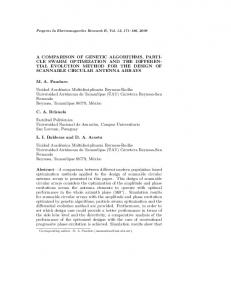
Fig. 1. Mixture of Gaussians derived from the EM algorithm (in a scale 0-8) for inactive (a), walking (b) and running (c). Mixture of Gaussians derived from the GA algorithm (in a scale 0-0.3) for inactive (d), walking (e) and running (f).
The next table show the confusion matrix for the EM and the GA where each column of the matrix represents the instances in a predicted class, while each row represents the instances in an actual class.
5 Discussion The results show a clear better performance for the GA over the EM algorithm. Furthermore, the EM algorithm does not take advantage of having two Gaussian distributions per state and merges both functions in only one. The EM inferred a Gaussian that classifies 90 out 91 running samples in a correct way, but paying the high price of misclassifying 269 walking samples as running. Nevertheless, the genetic algorithm enhances the total classification by ignoring the running samples and classified in a cored way 453 walking samples out of 454. As we can see in the pictures of the Gaussians, the EM inferred a great peak for the inactive activity, in contrast with the low probability assigned to the running state. On the other hand, the GA creates a small probability for the inactivity. In fact, the first mode of the Gaussian for the inactive state is centred in (0.5322, 0.2755) with a small weight of 0.5876. The second mode is centred in (2.3928, 0.8261) and a weight of 2.11. Nevertheless, the GA creates a high probability distribution for the walking state with two Gaussian centred in (2.0002, 2.2480) and (2.7381, 1.0947) and weight of 3 and 4 respectively. Moreover, the result of the classification by using EM is greatly dependant on the initialisation of the parameters in contrast to the GA that give stable results independently of the initial values. As a conclusion, we can derive that for this case the GA outperforms the traditional EM at the expense of ignoring the running activity. Thus, for real applications, a trade-off must be done according to the results that we are interested in obtaining.
406
Ó. Pérez et al.
References 1. Moeslund, T.B. and Granum, E. ‘A Survey of Computer Vision-Based Human Motion Capture’. Computer Vision and Image Understanding, Volume 81(3), 2001, pp. 231 – 268. 2. Pavlidis, I., Morellas, V., Tsiamyrtzis, P., and Harp, S. ‘Urban surveillance systems: from the laboratory to the commercial world’, Proc. IEEE, 2001, 89, (10), pp. 1478–1495. 3. Rath, T.M., and Manmatha, R.: ‘Features for word spotting in historical manuscripts’. Proc. of the 7th Int. Conf. on Document Analysis and Recognition, 2003, pp. 512–527. 4. Oates, T., Schmill, M.D., and Cohen, P.R.: ‘A method for clustering the experiences of a mobile robot with human judgements’. Proc. of the 17th National Conf. on Artificial Intelligence and Twelfth Conf. on Innovative Applications of Artificial Intelligence, AAAI Press, 2000, pp. 846–851. 5. Yamato, J., Ohya, J., and Ishii, K., ‘Recognizing human action in time-sequential images using hidden Markov model,’ Proceedings of CVPR '92, pp. 379-385. 6. Wilson, A.D. and Bobick, A.F., ‘Parametric hidden Markov models for gesture recognition’, IEEE Transactions on Pattern Analysis and Machine Intelligence, 1999, 21, (9), pp. 884 – 900. 7. Bicego, M. and Murino, V., ‘Investigating hidden Markov models' capabilities in 2D shape classification,’ IEEE Transactions on Pattern Analysis and Machine Intelligence, 2004, 26, (2), pp. 281 – 286. 8. Nguyen, N.T., Bui, H.H., Venkatesh, S., and West, G.: ‘Recognising and monitoring highlevel behaviour in complex spatial environments’. IEEE Int. Conf. on Computer Vision and Pattern Recognition, Wisconsin, 2003, pp. 1–6. 9. Rota, N. and Thonnat, M. ‘Activity Recognition from Video Sequences using Declarative Models’, Proc. European Conf. on A.I., 2002, pp. 673 – 680. 10. Stamp M ‘A Revealing Introduction to Hidden Markov Models’ January 18, 2004, http://www.cs.sjsu.edu/faculty/stamp/RUA/HMM.pdf. 11. Bilmes, J. 1998. A gentle tutorial on the EM algorithm and its application to parameter estimation for Gaussian mixture and Hidden Markov Models. Tech. Rep. ICSI-TR-97-021, University of California Berkeley. 12. http://homepages.inf.ed.ac.uk/rbf/CAVIAR/caviar.htm 13. http://www.cs.ubc.ca/~murphyk/Software/HMM/hmm.html 14. http://www.shef.ac.uk/acse/research/ecrg/gat.html