way to represent common code structures like loops and if- then-else constructs. This paper focuses on the flow diagrams and describes a method for generating ...
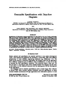
Compilation of Flow Diagrams into Target Code for Embedded Systems Achim Rettberg, Edwin Erpenbach, Jürgen Tacken, Carsten Rust, Bernd Kleinjohann C-LAB, 33095 Paderborn-Germany Tel: +49 5251 606110, Fax: +49 5251 606065 Email: {achcad, edwin, theo, car, bernd}@c-lab.de Abstract In this paper we describe a part of our work on the automatic generation of target code from Stateflow models. We focus on the flow diagrams from the Stateflow component of MATLAB and describe how flow diagram models can be compiled into target code for embedded systems. Moreover, the paper describes a method for analyzing flow diagrams, allowing an efficient code generation. The method described has been implemented as a code generator for Stateflow models and integrated into the TargetLink environment from dSPACE [3, 4].
1
Introduction
Complex embedded systems are easier to design at a high abstraction level. State-transition diagrams have shown to be very adequate for such high level modeling tasks. In such high-level models, many aspects, time in particular are handled in a quite abstract fashion, allowing a design that is not dependent of the target architecture. As state-transition diagrams also form an executable specification means, functional aspects of a system under development can be analyzed through simulation or rapid prototyping in very early design phases. Even if merely used for specification purposes, the use of state-transition diagrams hereby offers many advantages compared to a manual realization from the very beginning. But there is also an increasing demand to automatically translate executable specifications into a target specific implementation, i.e. to have a closed design chain. Only in this case design changes can directly be propagated down to the target architecture, reuse of specification parts becomes feasible and design cycles are likely to be shortened considerably. Although state-transition diagrams have shown to be well suited for automatic compilation, specific target architectures, especially those with limited computational and memory resources as they are commonly used within embedded systems, are not generally addressed In this paper, we focus on the component Stateflow of the MATLAB environment [6], which provides a powerful means for specifying embedded systems. MATLAB is a widespread tool, and its component Stateflow allows the modeling of reactive systems with state-transition diagrams similar to statecharts [5, 2]. A Stateflow diagram is a graphical representation of a finite state machine where states and transitions form the basic building blocks of the system. Stateflow however
also allows the representation of flow diagrams which are stateless. Flow diagram notation is essentially logic, represented without the use of states and is an effective way to represent common code structures like loops and ifthen-else constructs. This paper focuses on the flow diagrams and describes a method for generating efficient code from such models. The method presented in this paper includes the following steps: 1. A control flow graph is generated from the given flow diagram. 2. Taking the semantics of stateflow into account, a set of transformations are performed on the model in order to reduce the number of transitions as far as possible. 3. Finally, the remaining transitions are compiled into Ccode. The paper is organized as follows: the next Section describes the structure and semantics of the models we consider in this paper. Section 3 describes the compilation process, the transformation steps used to simplify the models and the transformation algorithm. Finally, an example is presented in Section 4.
2
Stateflow Models
Stateflow diagrams consist of hierarchical state diagrams (charts) and data elements that can flow between them. A system described by a Stateflow diagram has a set of external input and output data-elements, and a set of local data-elements (Figure 1). Each chart consists of a set of hierarchical states, a set of connective junctions (connectors) and a set of transitions between the states and the connectors. Each transition has a label of the form e[c]{a}/a’, where e is the event triggering the transition, c is the condition guarding the transition, a is the action and a’ is the transition action executed evaluating the transition, respectively. In Figure 1, we see an example model with two inputs i1, i2 and one output o1. The semantic of the Stateflow model is described in detail in [6]. The differences between the event and condition of a transition is, that events drive the charts execution and makes an recursive call of the system. A condition only represents a boolean expression, that must be true for the transition to be executed. The differences between the action and transition action is described in [6], but it is not relevant for our approach.
3
Transformation steps
In this chapter we describe the transformation steps. We distinguish between two types of transformation. The transformations belonging to the first type consider both the flowchart graph and the annotations of the transition. They will be described in Section 3.1-3.4. The other transformations consider only the flowchart graph and make some structural modifications. These transformations will be described in Section 3.5. To simplify the description of the transformation steps we use only actions in the annotations of the transition. The transformations however apply as well for transitions also containing transition actions.
3.1 Figure 1: Stateflow model with a flowchart
In our approach, we focus on the code generation for flowcharts. Flowcharts consist only of transitions and connectors and not states. The state ‘Adjust’ in Figure 1 triggered by the event compute contains a typical flowchart. It consists of two connectors and three transitions. There exists a loop between connector 1 and 2, because connector 1 has an outgoing transition to connector 2 and the other way round. The action annotating the first transition is ‘i = 0’. The annotation from the transition, which connects the connectors 2 and 1 consists of a condition (‘i < 10’) and an action (‘i++’). Taking these annotations and the structural information of the flowchart into account, it follows that the flowchart implements a typical for loop: for(i = 0; i < 10; i++) { out = i * out; } It is possible to use the code generation component of Stateflow (the Stateflow Coder) in order to generate C code. The generated code from the Stateflow Coder includes marks for the connectors, and the transitions are implemented by goto-jumps. This basic approach follows the direct propagation of a flowchart to C code. But this code is not well structured and it is very hard to find equivalencies between the model and the C code. In our approach we have a concept to look globally on the flowchart. The advantage of our method is that special control structures, e.g. loops can be identified. Since our code generation is done with respect to these structures, the resulting code is more compact and well structured. The following Section describes our set of transformations for various control structures. The transformations are similar to standard compiler optimizations [1].
Definitions
The following definitions will facilitate the description of the transformation steps: • Let G = (V, E) be a flowchart, where V is the set of connectors (vertices) and E the set of transitions (edges). Let k ∈ V be a connector, and t ∈ E a transition in the flowchart. • Furthermore, let TRANS(k, k’) := ∃ k, k’ ∈ K: grad(k) - #{(k, k’)} = 1, whereby grad(k) represents the degree of k and #{(k, k’)} is the number of transitions between k and k’. • Let in(k) and out(k) be the number of input and output transitions of the connector k. • A connector is simple if it has only one input and output transition. • For a transition t ∈ {(k, k’)}, let source(t) = k and dest(t) = k’ be the source and the destination connector of t respectively.
3.2
Sequence Transformation
This transformation could be performed for each simple connector, i.e. each connector having exactly one input and output transition (connector 1 in Figure 2 for example). SEQUENCE(k):= in(k) = out(k) = 1 The sequence transformation will be executed as follows. We delete the simple connector and its outgoing transition. The annotations from this transition will be assembled with the annotations from the incoming transition of the simple connector. There are miscellaneous forms to assemble the annotations. One example is depicted in Figure 2, the action A1 and A2 will be merged in serial. Finally the incoming transition of the simple connector will be linked to the following connector. In Figure 2 is this the connector 2.
3.4
If-then Transformation
The if-then transformation is similar to the or transformation, and applies to connectors with at least two output transitions all having the same destination connector. All output transitions must be annotated with an action. Furthermore at most one transition may have neither an event nor a condition (see Figure 4).
Figure 2: Sequence transformation
3.3
IF-THEN(k, k’):= out(k) > 1 and ∀ t ∈ T: source(t) = k ⇒ dest(t) = k’ and ∃ t ∈ T: source(t) = k ⇒ condition(t) ≠ φ or event(t) ≠ φ and ∃ t ∈ T: source (t) = k ⇒ action(t) ≠ φ or transition_action(t) = φ
Or Transformation
The or transformation applies to connectors with at least two outgoing transitions. The annotations of these outgoing transitions may only contain conditions or events. If one transition has an action or transition action, the or transformation cannot be used. Furthermore all outgoing transitions must have the same destination connector. OR(k, k’):= out(k) > 1 and ∀ t ∈ T: source(t) = k ⇒ dest(t) = k’ and condition(t) ≠ φ or event(t) ≠ φ and action(t) = φ and transition_action(t) = φ When the requirements are fulfilled the transformation works as follows. The transitions between the two considered connectors are combined to a single transition labeled with the corresponding events and conditions. Figure 3 shows an example of an or transformation, where the events and conditions were separately combined with an or conjunction and stored at one transition. Subsequently, a sequence transformation can be performed.
Figure 4: If-then transformation example
The transformation works as follows. Each transition except one will be compiled into an if-then construct, whereas the condition of the if statement contains the condition and/or event from the transition annotation. If the annotation of the transition contains both, they will be combined with an and conjunction. The action annotation of the transition will be mapped after the then statement of the if construct. Finally, the different if-then constructs are concatenated to an if-then-else cascade labeling a single transition. At this point a sequence transformation might possibly be performed.
3.5
Loop Transformation
The loop transformation applies to a connector k with exactly two input transitions and one output transition. In Figure 5 is this connector 1. Furthermore, the so called back transition must contain a condition. The back transition and the only outgoing transitions from connector k are linked to the same connector k’. The back transition condition represents the loop condition. By the transformation the back transition will be deleted and the annotations will be combined with the annotations of the only output transition of the connector. Figure 3: Or transformation example
LOOP(k, k’):= in(k) = 2 and out(k) = 1 and ∃ t ∈ T: source(t) = k ⇒ dest(t) = k’ and transition_action(t) = φ and ∃ t ∈ T: dest(t) = k ⇒ source(t) = k’ and condition(t) ≠ φ and event(t) = φ In Figure 5 the algorithm builds a while loop but it is also possible to build a for or a do-while loop. This depends on the annotations of the transitions. For example, for a for loop it is necessary to find an initialization and an increment statement. Figure 6: Split transformation example
Another form of splitting connectors is shown in Figure 7. This split method leads to the graph structure for the loop transformation described in Section 3.5.
Figure 5: Loop transformation example
Finally, similarly to the or and if-then transformation, a sequence transformation can be executed.
3.6
Structural Transformation
Flowcharts often include structures which cannot be transformed directly with the methods described above. In such cases it is necessary to transform the flowchart graph on a structural basis, using the transformations split and special split.
Figure 7: Another split transformation example
The special split is shown in Figure 8. It operates on two connectors k and k’ which are connected by at least two transitions. A new connector k’’ and a transition linking k and k’’ are inserted. Outgoing transitions between k and k’ are moved to k’’ and k’.
SPLIT(k):= in(k) > 1 and out(k) > 1 SPECIAL-SPLIT(k, k’):= in(k) > 1 and out(k) > 1 and ∃ t1 ... tn, n > 1: source(ti) = k ⇒ dest(ti) = k’ Connector 1 in Figure 6 has more than two incoming and outgoing transitions. None of the transformation methods described before can be used. But when we split the connector 1 into two connectors, one with the ingoing transitions and the other with the outgoing transitions and insert a new transition, a transformation can be applied. Since the inserted transition has no annotation, the semantical meaning of the flowchart remains unchanged.
Figure 8: Special split transformation
3.7
Transformation-Algorithm
In this Section we describe the transformation algorithm. The algorithm ensures the order of the above
described transformations, and operates on a graph G = (V, E) as introduced in Section 3.1. Algorithm: 1: while [ (#K > 1) && (∃ k, k’ ∈ K: TRANS(k, k’)) ] 2: { if (∃ k ∈ K : SEQUENCE(k)) 3: then make a sequence transformation for k 4: else 5: { if (∃ k, k’ ∈ K : OR(k, k’)) 6: then make an or transformation for k, k’ 7: else 8: { find k, k’ ∈ K: TRANS(k, k’) 9: if (∃ k, k’ ∈ K: IF-THEN(k, k’)) 10: then make an if-then transf. for k, k’ 11: else 12: { if (∃ k, k’ ∈ K: LOOP(k, k’)) 13: then make a loop transf. for k, k’ 14: else 15: { if (∃ k ∈ K: SPLIT(k)) 16: then make a split transf. for k 17: else 18: { if (∃ k, k’ ∈ K: SPECIAL-SPLIT(k, k’)) 19: then make a spec. split transf. for k, k’ 20: else get next k; 21: } 22: } 23: } 24: } 25: } 26:}
4
Example
The following example in Figure 9 illustrates a typical cycle for the code generation. Starting from the original model in Figure 9 a) the code generation algorithm performs a split transformation for connector 1, leading to the situation depicted in Figure 9 b). This step is followed by an if-then transformation for connector 3 (Figure 9 c)). Afterwards it is possible to make a sequence transformation for connector 3. The transition annotation between connector 1 and 2 then contains an if-then-else statement, see Figure 9 d). At this point, a loop transformation for connector 1 may be used (Figure 9 e)). The transition annotations contains first the if-then-else statement and then a while loop which contains again the if-then-else statement and the action A3. The condition C3 becomes the condition of the while loop. Finally, the code generation algorithm executes a sequence transformation for connector 1. At this time the algorithm ends, because there is only one transition and one connector remaining in the flowchart.
5
Conclusion
In this paper we have presented a method for generating efficient C code for flowcharts in a Stateflow model. We
explained how complex control structures can be recognized and compiled into efficient target code. The presented method is such that the specified structures are easy to recognize in the generated code.
Figure 9: Example
Acknowledgments The presented method has been integrated into the commercial tool TargetLink from dSPACE [3, 4]. The authors would like to thank their colleagues from dSPACE, especially Mr. M. Meyer and Mr. C. Grascher.
References [1] A. Aho, R. Sethi, and J. Ullman, Compilers: Principles, Techniques and Tools, Addison-Wesley, 1986.
[2] E. Erpenbach, J. Stroop, F. J. Rammig, “On the Compilation of Statecharts Models into Target Code for Embedded Systems”, in Proceedings IEEE Conference on Control Applications, 1999 [3] H. Hanselmann, “Development Speed-Up for Electronic Control Systems”, Convergence International Congress on Transportation Electronics, Dearborn, USA, October, 1921, 1998
[4] H. Hanselmann, U. Kiffmeier, L. Köster, M. Meyer, “Automatic Generation of Production Quality Code for ECUs”, SAE Congress ’99, Detroit, USA, March 1-4, 1999 [5] D. Harel, A. Naamad, “The STATEMATE semantics of statecharts”, ACM Trans. Soft. Eng. Method. Oct. 1996.. [6] The MathWorks Inc, Stateflow User’s Guide, 1999.