Complete Calibration of a Multi-camera Network. Patrick Baker and Yiannis Aloimonos ...... [12] S. M. Seitz and K. N. Kutulakos. Plenoptic image editing. In. Proc.
Complete Calibration of a Multi-camera Network Patrick Baker and Yiannis Aloimonos Computer Vision Laboratory University of Maryland College Park, MD 20742-3275 E-mail: fpbaker, yiannisgcfar.umd.edu Abstract We describe a calibration procedure for a multi-camera rig. Consider a large number of synchronized cameras arranged in some space, for example, on the walls of a room looking inwards. It is not necessary for all the cameras to have a common field of view, as long as every camera is connected to every other camera through common fields of view. Switching off the lights and waving a wand with an LED at the end of it, we can capture a very large set of point correspondences (corresponding points are captured at the same time stamp). The correspondences are then used in a large, nonlinear eigenvalue minimization routine whose basis is the epipolar constraint. The eigenvalue matrix encapsulates all points correspondences between every pair of cameras in a way that minimizing the smallest eigenvalue results in the projection matrices, to within a single perspective transformation. In a second step, given additional data from waving a rod with two LEDs (one at each end) the full projection matrices are calculated. The method is extremely accurate—the reprojections of the reconstructed points were within a pixel.
1. Introduction In this paper, it is shown how to obtain the projection matrices for M cameras given N points, each projected into a subset of the M cameras. The calibration method uses every correspondence between every camera in a unified framework, based on an error measure which operates over all the camera correspondences at the same time. The calibration scheme is easy to implement for any number of cameras and requires no user intervention after the initial data collection. The past few years have seen some work in computer vision conducted in a multi-view environment (for example, work on image based rendering [12], multi-view structure from
motion [11], multi-view human motion capture systems and multi-view virtualized reality [10]). In order for such techniques and the ones that will follow to produce accurate results, an accurate calibration is required. The basic method calculates the projection matrices for all cameras to within a single perspective transformation. An extension to the scheme calculates the full projection matrices given additional input data, such as images of a line segment (rod) of known length, or the image of a calibration frame from two cameras. This method is applicable to the calibration of large complexes of linear projective cameras of varying internal and external parameters. This method ensures that all the cameras are calibrated as a single instrument so that methods such as voxel carving and various algorithms in surveillance and monitoring can be implemented with maximal accuracy.
1.1. Contributions of the work and new ideas The calibration procedure described here is a form of a multiframe structure from motion algorithm based on point correspondences, which are, by construction, of accuracy to within a pixel. The technique itself has a number of novelties as will become clear in the sequel, but there exist two innovations that make the procedure very robust and of general applicability. First, not all points need to be visible by all cameras simultaneously. This makes it possible to calibrate camera networks of unrestricted topologies, such as the following (Figures 1, 2 and 3). Figure 1 shows a map (blue print) of the corridors of a building floor with clusters of cameras placed at intervals along the walls. The technique described here can be used for calibrating this network. Figure 2a shows cameras arranged on the walls of a room and Figure 2b shows cameras arranged in a dome configuration. Our technique can be used here. Finally, Figure 3 shows a network of cameras looking outwards and arranged in some small volume of space. Our technique can be used
here as well, but we would need to have the system in Figure 3 surrounded by other cameras, for example, by putting it in the room in Figure 2a or in the dome of Figure 2b. This way, we acquire information about the relative location of two cameras without a common field of view by relating them to surrounding cameras. The second innovation of the approach stems from a series of recent theoretical results in structure from motion. It has been shown [2, 3] that when a whole field of view (360 degrees) is available, the problem of recovering 3D motion and structure does not have the ambiguities and instabilities present in the case of a restricted field of view. Thus, in calibrating a multi-camera network we make sure that the collective field of view is such that it spans the whole space surrounding the area of interest. When, due to the topology of the network this is not possible, we use auxiliary cameras to achieve the full field effect. For example, consider that you wish to calibrate a stereo system. You could use three cameras (as in Figure 4) and perform the calibration procedure described here by waving a light in the space between the cameras. The outcome will be a robust calibration of the whole system and thus of the stereo system as well.
(a)
(b) Figure 2. (a) Camera network in a room. (b) Dome-shaped camera network.
Figure 1. Camera network in a hallway.
1.2. Previous work Previous calibration work has concentrated on the calibration of one camera with respect to a fixed reference calibration pattern, such as in [4]. One notable paper is [9] in which they ask if an accurate calibration pattern is really necessary. They answer their question in the negative through the use of at least three or more views from the same
camera and simultaneous estimation of point location and calibration. They are also not concerned with external, but only internal calibration. Calibration of three views has also been accomplished through the use of trilinear constraints [6, 13, 15] or quadrilinear constraints [6, 8, 15], but these tools are not well suited to the problem of calibrating many cameras at the same time. Spetsakis offers a solution in [14], but his algorithm uses only calibrated cameras, and additionally does not obtain the full projection matrices, even for calibrated cameras.
2.2. Input data The fact that the cameras are synchronized and that the lights can be turned off allows for many point correspondences. A calibrator waves around a rod with an LED on the end of it. The algorithm uses simple background subtraction and thresholding to extract the points. The correspondences are then used in a large nonlinear eigenvalue minimization routine, the basis of which is the epipolar constraint. The eigenvalue matrix encapsulates all the point correspondences between every pair of cameras in a way that minimizing the smallest eigenvalue results in the projection matrices.
3. Mathematical preliminaries Figure 3. A compound-like eye composed of conventional video cameras.
3.1. Notation All vectors are column vectors, and transpose is used wherever necessary to keep the equations consistent. This is especially important in using the technique presented here, since many matrix morphology operators are used and a convention avoids confusion. An m � n matrix A is represented as row vectors 2
aT1 3 6 aT 7 6 27
A = 64
Stereo system
Auxiliary cameras Figure 4. Scheme to calibrate a stereo system.
2. A multi-camera laboratory 2.1. Motivation The motivation for the work in this paper came with the construction of several multi-camera laboratories all over the world. For a laboratory like that, see Figure 5. There are 64 cameras placed on the walls around the room. The cameras can be moved and refocused, so that calibration is needed with every data set. The cameras are synchronized, so that each frame in all cameras is taken at precisely the same time. It would be time consuming to locate the points of a calibration grid for each of the 64 cameras every time data is required. A calibration method with little to no user intervention is required.
a
where each i is an n vector.
.. 7 . 5
aTm
A may also be represented as 3 �1;1 �1;2 : : : �1;n 6 �2;1 �2;2 : : : �2;n 7 7 6 2
A = 64
.. .
.. .
..
.
.. 7 . 5
�m;1 �m;2 : : : �m;n
3.2. Projective model Using the standard projective model, a world point Q can be projected onto the image plane of an arbitrarily positioned unnormalized projective camera. Homogeneous coordinates represent = [X Y Z 1]T and the projection can be modeled with a 3 � 4 matrix P which takes a homogeneous 3-vector and transforms it into a homogeneous 2-vector P = = s [x y 1]T . P can be factored into the standard matrices K , R and T by using the QR decomposition to obtain P = KR [I3 j ], where K is upper triangular, R is a rotation matrix, and is a 3-vector. Note that contrary to convention, the camera is translated first then rotated. This is a necessary convention for this algorithm to work. These form the standard translation, rotation, and projection matrices. In the sequel, K and
Q
Q q
Q
T T
Figure 5. A panorama of a multi-camera laboratory
R separately will not concern us, and instead B
= KR is used. Since the input to the algorithm is essentially a point cloud with no metric information, it is only possible to obtain calibration to within a 4 � 4 perspective projection H (see Theorem 1 in [5]), where
u0vT ]s =[AuvT ]s =[Au[v1 v2 v3 ]]s 2 3 Auv1 = 4Auv2 5 Auv3
[
Pi H = Pi�
2
uv13 = 4 0 A 0 5 � 4uv2 5 0 0 A uv3 T =[A]� [uv ]s A
Interestingly, ground control points are not needed in order find this H to within a conformal mapping. Only some sort of metric information must be specified. This metric information can be supplied by a wand with lights on both ends. The constant distance between the lights will calibrate the entire system to within a scale factor. If the distance between the lights is measured, then the scale factor is specified as well. This technique has the added benefit of being highly redundant so that distances are equalized throughout the entire camera field of view.
3.3. Morphology operators Morphology operators which operate on 3 � 3 matrices are necessary for the derivations. For any 3 � 3 matrix M , the stacking operator is defined as:
with it is defined as usual: 2
0 1 0 0 0 0 0 0 0
0 0 0 0 1 0 0 0 0
0 0 0 0 0 0 0 1 0
0 0 1 0 0 0 0 0 0
0 0 0 0 0 1 0 0 0
u
v
3
?v3 v2 0 ?v1 5
v�
[[ ] ]s =
2 3 03 ��21;;11 0 �3;1 7 07 6 �1;2 7 07 6 6 = D[M ]s 07 � 6�2;2 7 05 �3;2 7 4�1;3 5 0 0 �2;3 1 �3;3
Two 3-vectors and can form [ T ]s . Setting 0 = A , where A is any 3 � 3 matrix, results in the following identity:
u
0
0
Finally, note that
2
where
0 0 0 0 0 0 1 0 0
2
v0 = Av results in:
v � = 4 v3 ?v2 v1
The stack of a transpose of a matrix is as follows:
0 0 0 1 0 0 0 0 0
3
uv0T ]s =D[v0uT ]s T = D [A]� [vu ]s T = D [A]� D [uv ]s T =[A] [uv ]s where [�] = D[�]�D. Given a vector v, the skew symmetric matrix associated
2
[M T ]s = 2� 3 2 1;1 1 �1;2 0 6�1;37 60 6�2;17 60 6�2;27 = 60 6�2;37 40 4�3;15 0 0 �3;2 0 �3;3
0
where [�]� is defined here. Deriving another identity with
[ ]
m1 3 [M ]s = 4m2 5 m3
0
uv
u
K
6 6 6 6 6 6 =6 6 6 6 6 6 4
Kv
0
0
0
1 7 7
0
?177
0 0
?1
0
0
1
0
0
1
?1 0
0 0
0
3
0
0 7 7 0 7 7 0 7 7 0 7 7 0 5 0
These results will be used later in the paper.
4. Projective multiframe calibration
where Aj;k = K T A0j;k K . Equation 1 just states that j ? k is an eigenvector of Aj;k with zero eigenvalue. This condition in equation 1 will not hold in the presence of noisy data, but the least eigenvector (eigenvector associated with the least eigenvalue) of Aj;k should be the translation between cameras j and k. This idea can be extended to be useful for many cameras. Shown next is a technique for forming a matrix whose least eigenvector is the concatenation of all the camera positions = [ T1 T2 : : : TM ?1 ]T , where it is assumed without loss of generality that M = [0 0 0]T . To this end, form
T
T
4.1. Problem statement The camera system projects N 3D points, represented by
R1; R2; : : :; RN , onto M cameras, represented by projection matrices P1 ; P2; : : :; PM . A given point Ri is not necessarily projected onto camera j , but if it is, the projection is ri;j = Pj Ri . If a particular point Ri does not project to a camera j , then ri;j = [0 0 0]T for notational convenience. The algorithm should output, given the points r, the matrices Pj for all j . Since the camera system is calibrated using the LED method, it is assumed that there are many accurate point correspondences, so that minimality and robustness of data is not a concern. What is a concern is using all of the correspondences in an integrated minimization routine, so that all of the cameras are calibrated at one time.
4.2. Solution framework Given the set of points r�i;j in cameras j , the algorithm searches for those matrices Bj?1 such that the ri;j = � are effectively formed in cameras which are B ?1 vecri;j
j
only translations apart from each other. That is, all cameras have projection matrices of the form Pj = [I3 j i ]. The algorithm measures this with the epipolar constraint, assuming that all the cameras are only translations apart from each other. Thus the algorithm can be seen as putting all the cameras into the translated copies of the same coordinate frame.
T T T
T
2
A1;1+i
Ai
6 6 6 6 =6 6 6 6 4
T
3
A2;2+i
..
.
AM ?i;M
..
.
AM;i
7 7 7 7 7 7 7 7 5
which is a block diagonal matrix containing the 3 � 3 epipolar constraints for all the cameras which are i indices apart, and zeros elsewhere. Given the 3M � 3M shift matrix 2
T
4.3. Normalized cameras
T
SM
0
60 6 6 =6 6 40
I3 0
.. .
::: I3 : : : 0
..
.
0
3
07 7
.. 7 .7 7
: : : I35 I3 0 0 : : : 0 Li;M is defined to be the left 3M � 3(M ? 1) submatrix of i . Li;M is constructed so that T is in the nullspace I3M ? SM 0
0
of For the first derivation, it is assumed that all our cameras have projection matrices of the form Pj = [I3 j i ]. This may seem to be an unnatural restriction, but the results will be extended later to general projection matrices. Every pair of cameras j and k is constrained to have the sum of the squares of the epipolar constraint be zero. Simplified by the lack of rotation assumption, this is:
T
X
i Setting
rTi;j [Tj ? Tk ]�ri;k )2 = 0 X
i
The method to calibrate the cameras is to find those matrices Bj , such that setting
ri;jrTi;k ]s[ri;j rTi;k ]Ts
ri;j = Bj?1 r�i;j
[
the above is equivalent to:
Tj ? Tk ]�]Ts A0j;k [[Ti ? Tk ]� ]s = 0 T T 0 (Tj ? Tk ) K Aj;k K (Tj ? Tk ) = 0 T (Tj ? Tk ) Aj;k (Tj ? Tk ) = 0
T
section is , if the cameras are in general position (no four coplanar). The constraint that C has one zero eigenvector is a constraint on all the correspondences among all cameras.
4.4. Calibrating the cameras
(
A0j;k =
Ci = LTi Ai Li P The null space of C = i Ci will be the intersection of the null spaces of the Ci. The only vector in this inter-
[[
(1)
where the star denotes the originally measured points, results in the C matrix constructed from the Bj having an eigenvalue close to zero. A nonlinear minimization over the Bj will minimize the smallest eigenvalue of C . By using the previously derived morphological identities, it can be shown there is no need to multiply all the
points to form A0j;k at every iteration. It is sufficient to multiply the A0j;k as follows. P T ]s[ri;j rT ]T A0j;k = i [ri;j ri;k i;k s P ?1 � ?1 r� )T ]s[B ?1 r� (B ?1 r� )T ]Ts = [ B ( B r j i;j k i;k i j i;j k i;k ?1 ?P [r� r�T ]s[r� r�T ]Ts � [B ?1 ]T [B ?1]T� ?1 = [Bj ]� [Bk ] i;j i;k k j i i;j i;k ?1 ?1 0 � ?1 T ?1 T = [Bj ]� [Bk ] A j;k [Bk ] [Bj ]� thus obtaining
Aj;k = K T A0j;k K ?1 0 � ?1 T ?1 T T ?1 = K [Bj ]� [Bk ] A j;k [Bk ] [Bj ]� K
The minimization can compute the smallest eigenvalue of C � over all of the Bi ’s using precomputed matrices A0j;k .
4.5. Extracting the B matrices from the fundamental matrix
h
� = U 01 0 = B2 [T ]�
0 0
�2
�
�
0 i ?v2TT � 0 ?v2 v1T �3 T
v1
� T� v1 v2TT T
� h1 0 0i T 0 1 0 0 0 0
with �3 arbitrary, and defining B2 . Thus setting �3 to a nonzero value will give us a nonsingular B2 compatible with the perspective projection chosen by setting B1 = I3 . Now given B1 and B2 which fix the perspective projection, the rest of the Bi , consistent with this perspective projection, can be found given F1;i and F2;i. Define
G0i = F1;iB1 = Bi?T [T1;i]� G00i = F2;iB2 = Bi?T [T2;i]� Taking the SVD of G0i results in: 2 32 3 �1 0 0 v1 T G0i = U 4 0 �2 05 4v2 T 5 0
0
0
TT
This result can be expanded as follows: The nonlinear minimization must have initial conditions reasonably close to optimal. Since it is not guaranteed that correspondences exist between more than two cameras, the only possibility is to use the fundamental matrices to somehow extract an estimate of our Bi matrices. The FMatrix program by Zhengyou Zhang [16] was used to generate good fundamental matrices for input. Given that as input, the following generates the Bi matrices. This factorization of the fundamental matrix is sufficient for our purposes. The fundamental matrix Fj;k is defined by T Fj;k i;j � 0 for all i. This can be factored as: i;k
r
r
Fj;k = Bk?T [Tk ? Tj ]� Bj?1
A single fundamental matrix is clearly not sufficient to extract any of the Bj ’s, but if it is only necessary to extract the Bj ’s to within a perspective transformation H , then all the Bj ’s can be obtained to within the same perspective transformation using only fundamental matrices. Since the B ’s only to within a perspective projection are necessary, it is necessary to fix 12 parameters (3 more are fixed by setting TM = [0 0 0] and the last one is a scale factor). Nine are fixed by setting B1 = I3 , and the three more parameters of B2 are fixed as follows. The fact that B1 = I3 implies F1;2 = B2?1 [T2 ? T1 ]� . It is noted here that the SVD of [T ]� is �
2 � 1 40
0
0
0
T � = ?v2 v1 T
[ ]
v v T
1
32
v1 T 3 05 4v2 T 5 0 TT 0
with 1 , 2 , mutually orthogonal. Now F1;2 can be decomposed using the SVD as follows, h� F1;2 = U 01
0
0 0
�2
�
0i v1TT 0 v2 0 TT
�
Bi?T [T1;i ]� = �� � � T �� h� � �T 0 0i v1 TT ?v2 U 01 �2 0 + TT v 2 0 0 1 0
TT
v1
� h1 0 0i T 0 1 0 0 0 0
� T� v1 T v2T T
Using the identity for [T ]� and taking the inverse transpose, results in: 2
? �11
Bi = U 4
0
0
32
3
05 4
v1T 5 wT
0
0
0
1
? �12
?v2T
where w is an unknown vector. Requiring BiT G00i to be skew
gives six linear conditions on w, which can be solved by least squares to get Bi . The result is the B1 , B2 , and Bi , which are all consistent with our three fundamental matrices. All the Bi can thus be used as initial conditions in the nonlinear minimization.
4.6. Obtaining the projection matrices Note that the nonlinear minimization is actually carried out on the Bi . The Ti are extracted from the least eigenvector when the minimization is complete. The projection matrices are then completed as:
Pi = [Bi j Bi � Ti ] 4.7. Algorithm overview Input.
M The number of cameras N The number of points r^i;j The corresponding points with 1 � i � M j � N.
and 1
�
Output.
M projection matrices Pi
g
Steps.
� �
Find the initial matrices Bi using Section 4.5
� �
From C � , calculate the least eigenvector T � .
Using the Bi?1 as initial conditions, minimize the smallest eigenvalue of C to obtain the optimal Bi� and C �. Using the Bi� and T � , calculate
Pi = [Bi� Bi� Ti� ]
d d
T parameters for a rotation R are = [d1d2 d3 ] , then the Soma parameters are = s[1 T ]T , with s a scale so that has length 1. Given unit , [1] shows that R can be expressed as
g
g
R= " 2 # g0 + g12 ? g22 ? g32 2(g1 g2 ? g0 g3 ) 2(g1 g3 + g0 g2 ) 2 2 2 2 2(g2 g1 + g0 g3 ) g0 ? g1 + g2 ? g3 2(g2 g3 ? g0 g1 ) 2(g3 g1 ? g0 g2 ) 2(g3 g2 + g0 g1 ) g02 ? g12 ? g22 + g32 6. Implementation details
� 0] PM = [BM
5. Extensions
This algorithm has been implemented in Matlab. Some implementation details which improve the performance of the algorithm follow.
5.1. Full multiframe calibration
6.1. Derivative of the C matrix
The execution of the algorithm described above results in projection matrices Pi, which are related to the actual projection matrices Pi� by Pi� = PiH , where H is a 4 � 4 matrix. To find H , a wand with lights on both ends is used. Using the Pi , world points Rj;m with m 2 f1; 2g can be reconstructed such that R�j = H ?1 Rj;m. Since the wand does not change in length over the course of a data acquisition session, it is known that the distance between R�j;1 and R�j;2 is constant. Since the points are in homogeneous coordinates, one can formulate the condition on H ?1 as follows. H ?1 R 1??3 j;1 ?1 H4 Rj; 1
2
?1 Rj;2 3 ? HH1???1 Rj; 2 4
=1
1 is the first three rows of H ?1 while H ?1 is the where H1??? 3 4 last row of H ?1 . This condition can be used in a nonlinear optimization in order to find H . 5.2. Self calibration
The Bj?1 which minimize the smallest eigenvalue of C are what is desired. A nonlinear optimization over the elements of Bj?1 for this smallest eigenvalue will obtain these parameters. To improve speed, it is possible to analytically take the derivative of the smallest eigenvalue of the C matrix with respect to each of the elements of the matrices Bj?1 . One just expands the sum which defines C and takes the derivative with respect to each matrix element in Bj?1 .
6.2. Preprocessing It was shown in [7] that it is helpful in calibration to have reasonable normalization for the image points. This algorithm is no exception. While a projective calibration is obtained, the stability of the algorithm is improved if a coarse estimate Ke ; j is made of the calibration matrix, for each j 2 [1; : : :; M ]. Then the algorithm operates on the 0i;j defined by
r
r0i;j = K ?1ri;j
6.3. Postprocessing To self-calibrate using this framework, it is assumed that there are correspondences from an uncalibrated camera with an unknown motion in a rigid environment. More precisely, this means that the Bi?1 can be decomposed as RTi K ?1 , with K not dependent on i. The nonlinear minimization can then operate over the 3M + 5 parameters defining the Bi?1 rather than the 8M parameters which define the Bi?1 up to scale. One technical difficulty with this approach is that in order to use an unconstrained minimization, the Ri must be parameterized. Rodrigues parameters [1] are not appropriate, because these parameters are infinite for half rotations. More appropriate is Study’s Soma [1], which is a homogeneous form of the Rodrigues parameters. If the Rodrigues
After the projection matrices are obtained, the calibration can be improved by reconstructing the world points, and then running a nonlinear optimization to obtain the projection matrices from the projections of the world points. The accuracy of the initial calibration, together with its selfconsistency, allows the execution of this procedure.
7. Calibration results The projective calibration algorithm has been implemented in Matlab, and has been used to calibrate a multicamera configuration consisting of 64 cameras capable of
synchronized recording. A typical data set contains approximately 2500 points, and each camera sees approximately half of those. It would be surprising if this method were not as accurate than a calibration frame, since it is possible to accurately locate corresponding points in every part of the cone of view of every camera. As long as the cones of view of the cameras intersect, then there should be sufficient data with which to calibrate. In the experiments, it was determined that the reprojections of the reconstructed points were within a pixel, which was the measurement error of the location of the LED.
8. Conclusion It has been shown that it is possible to calibrate a large system of cameras accurately with little user effort. This algorithm will be useful to calibrate a variety of multi-camera systems. In addition, as has been briefly explored here, the framework also allows for work on full Euclidean and selfcalibration of a moving camera.
References [1] O. Bottema and B. Roth. Theoretical Kinematics, chapter 6, pages 147–151. North-Holland Publishing Company, 1979. [2] C. Ferm¨uller and Y. Aloimonos. Geometry of eye design: Biology and technology. Technical Report CAR-TR-901, Center for Automation Research, University of Maryland, 1998. [3] C. Ferm¨uller and Y. Aloimonos. Observability of 3D motion. International Journal of Computer Vision, 1999. In press. [4] A. S. for Photogrammetry”. Manual of Photogrammetry, 4th edition. 1984. [5] R. Hartley, R. Gupta, and T. Chang. Stereo from uncalibrated cameras. In IEEE Computer Society Conference on Computer Vision and Pattern Recognition, pages 761–764. IEEE, 1992. [6] R. Hartley and A. Zisserman. Multiple View Geometry. Cambridge University Press, 1999. [7] R. I. Hartley. In defense of the eight-point algorithm. Pattern Analysis and Machine Intelligence, 19(6):580–593, June 1997. [8] A. Heyden. Geometry and Algebra of Multiple Projective Transformations. PhD thesis, Lund University, Sweden, December 1995. [9] J.-M. Lavest, M. Viala, and M. Dhome. Do we really need an accurate calibration pattern to achieve a reliable camera calibration. In 5th European Conference on Computer Vision, pages 158–174, 1998. [10] P. Narayanan, P. Rander, and T. Kanade. Constructing virtual worlds using dense stereo. In Proc. International Conference on Computer Vision, pages 3–10, Bombay, January 1998. [11] M. Pollefeys, R. Koch, and L. Van Gool. Self-calibration and metric reconstruction in spite of varying and unknown internal camera parameters. In Proc. International Conference on Computer Vision, pages 90–95, 1998.
[12] S. M. Seitz and K. N. Kutulakos. Plenoptic image editing. In Proc. International Conference on Computer Vision, pages 17–24, 1998. [13] M. Spetsakis and J. Aloimonos. A unified theory of structure from motion. In DARPA IU Workshop,pages 271–283, 1990. [14] M. Spetsakis and Y. Aloimonos. A multi-frame approach to visual motion perception. International Journalof Computer Vision, pages 245–255, 1991. [15] G. Xu and Z. Zhang. Epipolar Geometry in Stereo, Motion and Object Recognition: A Unified Approach. Kluwer Academic Publishers, 1996. [16] Z. Zhang. Determining the epipolar geometry and its uncertainty: A review. Technical Report 2927, INRIA, SophiaAntipolis, July 1996.