Completeness of monad-based dynamic logic. Till Mossakowski, Lutz Schröder, and Sergey Goncharov. DFKI Laboratory, Bremen, and. Department of ...
Completeness of monad-based dynamic logic Till Mossakowski, Lutz Schr¨oder, and Sergey Goncharov DFKI Laboratory, Bremen, and Department of Computer Science, University of Bremen
Abstract. Monads are used in functional programming as a means of modeling and encapsulating computational effects at an appropriate level of abstraction. In previous work, we have introduced monad-based dynamic logic and have used it for the specification and verification of various monadic functional-imperative algorithms over different monads. The semantics of this logic was originally defined over partial cartesian closed categories; completeness issues were explicitly left out of consideration. Here, we slightly simplify the logic and reformulate it in the weaker setting of a strong monad over a cartesian category with some additional infrastructure. We provide an extended proof calculus and prove its soundness and completeness.
The presence of computational effects, e.g. state, store, exceptions, input, output, non-determinism, or backtracking, substantially complicates reasoning about programs. Dealing with such features has in the past typically required dedicated logics, designed specifically for a particular combination of effects. As a unifying concept for modeling computational effects (in particular, all of those mentioned above) in an elegant way, monads, a well-known tool from category theory, have been established by Moggi in the seminal paper [5]. Based on this work, monads now form the basis of the treatment of encapsulated side effects in the functional programming language Haskell [11], which thanks to this concept admits clean programming in an imperative style. Monads have also appeared in programming semantics, e.g. for Java [3]. In previous work, we have introduced a monad-based Hoare calculus [9] and a dynamic logic [10] that allow reasoning about such generic effects. The semantics and proof calculus of both logics are parametrized over a monad (and hence, over a notion of side effect). The particular (combination of) effects needed for an application can then be axiomatically specified in the general framework. Monad-based dynamic logic (MDL) is similar to Pitts’ evaluation logic [7], but equipped with a rather different semantics which is induced directly by the underlying monad. So far, no completeness result has been proved for either of these logics. Here, we fill in this gap in the theory. We simplify MDL by detaching it from the HasCasl framework as used in [10]. Instead, we introduce a term language and semantics based on cartesian categories. The resulting calculus, slightly extended in relation to the calculus presented in [10], is shown to be
2
sound and complete by means of a term model construction; the main technical tool in the proof is a normalization procedure for dynamic formulae. Practical applications of MDL include reasoning about Haskell and Java programs. Numerous examples and a coding in the theorem prover Isabelle can be found in [12]. A Hoare calculus has been built on top of MDL [9] and extended to a treatment of Java-style abrupt termination [10, 13].
1
Monads for computations
On the basis of groundbreaking work by Moggi [5], monads are being used for encapsulating side effects in modern functional programming languages; in particular, this idea is one of the central concepts of Haskell [6]. Intuitively, a monad associates to each type A a type T A of computations of type A; a function with side effects that takes inputs of type A and returns values of type B is, then, just a function of type A → T B. This approach abstracts away from particular notions of computation such as store, non-determinism, non-termination etc.; a surprisingly large amount of reasoning can be carried without commitment to a particular type of side effect. A monad on a given category C can be defined as a Kleisli triple T = (T, η, ∗ ), where T : Ob C → Ob C is a function, the unit η is a family of morphisms ηA : A → T A, and ∗ assigns to each morphism f : A → T B a morphism f ∗ : T A → T B such that ∗ ηA = idT A ,
f ∗ ηA = f,
and
g ∗ f ∗ = (g ∗ f )∗ .
This description is equivalent to the more familiar one [4]. In order to support a language with finitary operations and multi-variable contexts (see below), one needs a further ingredient: a monad is called strong if it is equipped with a natural transformation tA,B : A × T B → T (A × B) called strength, subject to certain coherence conditions (see e.g. [5]). Example 1 ([5]). Computationally relevant monads on Set (all monads on Set are strong) include the following. – Stateful computations with possible non-termination: T A = (S →? (A×S)), where S is a fixed set of states and →? denotes the partial function type. A simple special case is the queue monad, where S = U ∗ for some alphabet U . – (Finite) non-determinism: T A = Pfin (A), where Pfin denotes the finite power set functor. – Exceptions: T A = A + E, where E is a fixed set of exceptions. – Interactive input: T A is the smallest fixed point of γ 7→ A + (U → γ), where U is a set of input values. – Non-deterministic stateful computations: T A = Pfin (S → (A × S)), where, again, S is a fixed set of states.
3
2
Dynamic logic
In program specification, dynamic logic as introduced in [8] and extended to monadic computations in [10] has a number of advantages over less expressive formalisms such as Hoare logic, among them the ability to express both partial and total correctness in a natural way and the possibility of reusing a state, say for statements of the nature ‘what would happen if’. Here, we examine the infrastructure that is needed in order to develop generic monad-based dynamic logic, and illustrate that this does indeed make sense when instantiated to typical concrete computational monads. Given a set S of basic types, the type system of monad-based dynamic logic (MDL) is generated by A ::= 1 | Ω | DA | T A | A × A | S. A signature Σ = (S, F ) consists of a set S of basic types and a set F of operation symbols f : A → B, where A and B are types over S. We make the general assumption that the operations in the signature have T -free argument types, i.e. types containing neither T nor D. The term language over a signature Σ and a context Γ of typed variables is given in Fig. 1. Repeated nestings such as do x1 ← p1 , . . . , xn ← pn ; q are somewhat inaccurately denoted in the form do x ¯ ← p¯; q. Term fragments of the form x ¯ ← p¯ are called program sequences.
(var)
x:A∈Γ Γ �x:A
(app)
(1)
Γ �∗:1
Γ �t:A×B Γ �t:A×B (snd) Γ � fst(t) : A Γ � snd(t) : A Γ �ϕ:Ω (⊥) (¬) similarly for ∧, ∨, ⇒, ⇐⇒ (>) Γ �>:Ω Γ �⊥:Ω Γ � ¬ϕ : Ω Γ � p : T A Γ, x : A � q : T B Γ � p : DA Γ, x : A � q : DB (do) (doD) Γ � do x ← p; q : T B Γ � do x ← p; q : DB Γ �t:A Γ � p : TΩ Γ � ϕ : DΩ (ret) (2) (MDL) Γ � ret t : DA Γ � 2p : DΩ Γ � ϕ : TΩ (pair)
Γ �t:A Γ �u:B Γ � ht, ui : A × B
f :A→B ∈Σ Γ �t:A Γ � f (t) : B (fst)
Fig. 1. Term language for propositional dynamic logic
The operations fst and snd are the projection functions for binary products. We treat n-ary products as iterated binary products; then projections πin can easily be defined in terms of fst and snd. The type T A contains the monadic programs over A; DA is a subtype of DA containing deterministically side-effect free programs. The type of booleans is denoted Ω; consequently, we take DΩ as the type of formulae of monad-based
4
dynamic logic. The term forming operation 2 : T Ω → DΩ is a closure operator. The formula 2p intuitively expresses that all terminating runs of p return >. Note that 2 does not behave like a modal operator; in particular, for ϕ : DΩ, we will have ϕ ⇐⇒ 2ϕ. However, 2 serves to define modalities: For ϕ : DΩ, we let [¯ x ← p¯] ϕ abbreviate the formula 2 do x ¯ ← p¯; ϕ, and omit the x ¯ if not occurring in ϕ. The formula h¯ x ← p¯iϕ abbreviates ¬[¯ x ← p¯] ¬ϕ. Both in do-terms and within modal operators, we implicitly identify terms up to α-equivalence. Besides the specification and verification of monadic programs, MDL serves also the specification of monads, i.e. notions of side effect. The running example of [9, 10] involves references and non-determinism; numerous further examples can be found in [12], including the Java monad and a parsing monad, as well as a queue monad over a set U of queue entries, axiomatized as follows using operations enq : U → T 1, deq : T U and mt : T Ω. 1. 2. 3. 4.
henq xi> [enq x]¬mt mt ⇒ [enq a; x ← deq](x = a ∧ mt) ¬mt ⇒ ([enq a; x ← deq](φ x) ⇐⇒ [x ← deq; enq a](φ x))
That is: 1. it is always possible to enqueue something, 2. after enqueueing, the queue is not empty, 3. for an empty queue, an enqueued element can be immediately dequeued again, and 4. for a non-empty queue, enqueueing and dequeueing one element do not interfere with each other (since both operations happen at the opposite ends of the queue). In combination with a specification of a reference monad, this specification has been used to implement and verify breadth-first search [12]. MDL is interpreted over a strong monad T on a cartesian category C with additional structure as follows. There is a distinguished object Ω such that homsets into Ω coherently carry a boolean algebra structure; i.e. the hom-functor hom( , Ω) factors through boolean algebras. We require that (idA × > : A × 1 → A × Ω, idA × ⊥ : A × 1 → A × Ω) is an episink. Moreover, T needs to be equipped with a strong submonad D; we require that DA consists of deterministically side-effect free computations as defined further below. Finally, we need a left inverse 2 : T Ω → DΩ of the inclusion DΩ ,→ T Ω. We then interpret the basic sorts as objects in C. This is easily extended to all types, giving an interpretation [[A]] for each type A. Basic operations f : A → B are interpreted as morphisms [[A]] → [[B]]. One then interprets terms x1 : A1 , . . . , xn : An � t : A as morphisms [[t]] : [[A1 × · · · × An ]] → [[A]], using the cartesian structure for pairing and projections, the monad for do and ret, and the boolean algebra structure on Ω for the boolean connectives as shown in Fig. 2. (Note that there is no particular rule for sequential composition within D: the fact that D is a submonad guarantees closedness under sequential composition.) Equations between terms are interpreted as equations between the corresponding morphisms. Remark 2. In a distributive category, one obtains the boolean algebra structure by defining Ω as 1 + 1. E.g., every topos is distributive, and in a classical topos,
5
(var) (app)
[[x1 : A1 , . . . , xn : An � xi : Ai ]] = πin
f : A → B ∈ Σ [[Γ � t : A]] = h [[Γ � f (t) : B]] = [[f ]] ◦ h (pair)
(fst)
[[Γ � > : Ω]] = >
[[Γ � ϕ : Ω]] = h (¬) [[Γ � ¬ϕ : Ω]] = ¬(h) (do)
(snd) (⊥)
[[Γ � t : A × B]] = h [[Γ � snd(t) : A]] = π2 ◦ h
[[Γ � ⊥ : Ω]] = ⊥
similarly for ∧, ∨, ⇒, ⇐⇒
[[Γ � p : T A]] = h1 [[Γ, x : A � q : T B]] = h2 [[Γ � do x ← p; q : T B]] = h∗2 ◦ t[[Γ ]],[[A]] ◦ hid, h1 i (ret)
(2)
[[Γ � ∗ : 1]] =!
[[Γ � t : A]] = h1 [[Γ � u : B]] = h2 [[Γ � ht, ui : A × B]] = hh1 , h2 i
[[Γ � t : A × B]] = h [[Γ � fst(t) : A]] = π1 ◦ h (>)
(1)
[[Γ � t : A]] = h [[Γ � ret t : DA]] = η[[A]] ◦ h
[[Γ � p : T Ω]] = h [[Γ � 2p : DΩ]] = 2 ◦ h
(MDL)
[[Γ � ϕ : DΩ]] = h [[Γ � ϕ : T Ω]] = ιΩ ◦ h
Fig. 2. Semantics of propositional dynamic logic
the subject classifier is just 1 + 1. In a category with equalizers, there is also a canonical choice for the subfunctor D, namely to take DA as the subobject of T A determined by deterministic side-effect freeness as defined below. Then the 2 arrow is uniquely determined if it exists (see Prop. 10 below). ¯ be contexts, let Γ � t¯ : B, ¯ Lemma 3 (Substitution). Let Γ and ∆ = y¯ : B and let ∆ � s : C. Then ¯ [[Γ � s[t¯/¯ y ] : C]] = [[∆ � s : C]] ◦ [[Γ � t¯ : B]]. MDL formulae will be interpreted as computations of type DΩ. They are expected to have no side-effect, although they may e.g. read the state (if a notion of state is present in the monad). This is abstractly captured as follows. Definition 4. A program p : T A is called discardable if (do y ← p; ret ∗) = ret ∗, and copyable if (do x ← p; y ← p; ret (x, y)) = do x ← p; ret (x, x). Finally, p is deterministically side-effect free (dsef ) if it is both discardable and copyable.
6
(In [10], we additionally require a commutation property. This is superfluous for simple monads, on which we focus here; cf. Prop. 21.) The equation for discardability can be interpreted as pair of arrows dis 0 , dis 1 : T [[A]] → T [[1]]; we require that ι[[A]] : D[[A]] → T [[A]] equalizes this pair. (We do not require that ι[[A]] is the equalizer, for the reconstruction of this equalizer in the term model would require a coercion of provably dsef terms of type T A to type DA, which means that term formation rules would need to interact with proof rules.) A similar requirement holds for copyability; i.e. we require that DA contains only dsef programs. We will want to regard programs that return truth values as formulae with side effects in a modal logic setting. A basic notion we need for such formulae is G : that of global validity, which we denote explicitly by a ‘global box’ � G ϕ abbreviates the equation Definition 5. Given a term ϕ : T Ω, �
ϕ = do ϕ; ret >. G ϕ simplifies to ϕ = ret >; otherwise, the equation If ϕ is discardable, then � above ensures that the right hand side has the same side-effect as ϕ. We say that G ϕ; this is usually an MDL formula ϕ is valid in a model T, and write T |= ϕ, if � expressed by just writing ϕ. As usual, by T |= Φ for a set Φ of MDL formulae we mean that T |= ϕ for all ϕ ∈ Φ, and by Φ |= ψ that T |= Φ implies T |= ψ for all T. A related notion is that of global dynamic judgements of the form [ x ¯ ← p¯] φ, which intuitively state that φ holds after x ¯ ← p¯, where φ : Ω is a truth-valued term in variables x ¯. The idea is to work with formulae that have all side effects shoved to the outside, so that the usual logical rules apply to the remaining part.
Definition 6. Given a program sequence x ¯ ← p¯ and a formula φ of type Ω, the notation [ x ¯ ← p¯] φ abbreviates the equation (do x ¯ ← p¯; ret h¯ x, φi) = do x ¯ ← p¯; ret h¯ x, >i. G do x Definition 7. A monad is called simple if � ¯ ← p¯; ret φ implies [ x ¯ ← p¯] φ.
(The converse implication holds universally.) Roughly, an algebraic monad [4] is simple if, in each of its equations, the two sides contain the same variables. All monads of Example 1 are simple. The continuation monad and the abelian group monad are not simple. In the sequel, all monads are assumed to be simple. Definition 8. T is said to admit dynamic logic, if for each q : T Ω and each x ¯ ← p¯ containing xi : Ω, [x ¯ ← p¯; a ← 2q]] (xi ⇒ a) iff [ x ¯ ← p¯; a ← q]] (xi ⇒ a). Proposition 9. If a simple monad T admits dynamic logic, then [x ¯ ← p¯; a ← [¯ y ← q¯] ϕ]] (xi ⇒ a) iff [ x ¯ ← p¯; y¯ ← q¯; a ← ϕ]] (xi ⇒ a), i.e. T admits dynamic logic in the sense of [10].
7
For ϕ, ψ : DΩ, let ϕ ≤ ψ if [ a ← ϕ; b ← ψ]] (a ⇒ b) This is easily seen to be a partial order. The following two claims are proved similarly as in [10]. Proposition 10. The formula 2p is the greatest formula ϕ : DΩ such that [ a ← ϕ; b ← p]] (a ⇒ b) Proposition 11. G [¯ [x ¯ ← p¯] φ iff � x ← p¯] ret φ
Proposition 10 implies that 2p is uniquely determined if it exists. Proposition 11 relates global dynamic judgements and local modal formulae. Note the difference between global dynamic judgements [ x ¯ ← p¯] φ and the similar-looking MDL formulae [¯ x ← p¯] ϕ involving a local modality. From a technical point of view, a global dynamic judgement is an equation between terms (and the component formula φ has type Ω), while a local modal formula is a term (and the component formula ϕ has type DΩ). But the difference is more fundamental: local modalities can be nested, and e.g. in the state monad one can think of them as being evaluated relative to a local state. This is not possible with global dynamic judgements: they always quantify over all states. Remark 12. As indicated above, MDL is similar to Pitts’ evaluation logic [7], but differs in several important respects. A minor syntactic difference is that evaluation logic includes equations, which could be added to MDL in later extensions. On the other hand, MDL allows unrestricted mixing of formulae and programs, as formulae are just programs with particular properties. Perhaps most importantly, the semantics of MDL arises uniquely from the underlying monad, while the semantics of evaluation logic depends on a hyperdoctrine which must in all likelihood be considered additional data (e.g. in the case of the state monad, the interpretation of formulae as state predicates is explicitly imposed by the chosen hyperdoctrine).
3
A Calculus for Dynamic Logic
Figure 3 shows a proof calculus for MDL. The calculus differs from the one in [10] in that the rules for the diamond are omitted, because in classical logic, 3 can be defined as ¬2¬. Moreover, Axioms (2), (dis), (copy), (unit) and (CC) have been added. The axiom schema (CC) throws in all equations CC ` t = u derivable using only the standard equations for tupling, projections, and ∗, i.e. the internal equations of cartesian categories. The usual logical connectives are lifted to DΩ by defining e.g. ϕ ⇒ ψ := [a ← ϕ; b ← ψ] ret (a ⇒ b) : DΩ,
8
which by (2MDL) below is equivalent to do a ← ϕ; b ← ψ; ret (a ⇒ b). We write Φ ` ψ if a formula is derivable in the calculus from a set Φ of axioms.
Rules: (nec)
ϕ x ¯ not free [¯ x ← p¯] ϕ in assumptions
(mp)
ϕ ⇒ ψ; ψ
ϕ
Axioms: (K) (seq2) (ctr2) (ret2) (dis) (copy) (cong-ret) (2) (unit) (CC) (taut)
[¯ x ← p¯] (ϕ ⇒ ψ) ⇒ [¯ x ← p¯] ϕ ⇒ [¯ x ← p¯] ψ [¯ x ← p¯; y ← q] ϕ ⇐⇒ [¯ x ← p¯] [y ← q] ϕ [x ← p; y ← q] ϕ ⇐⇒ [y ← (do x ← p; q)] ϕ [x ← ret t] ϕ ⇐⇒ ϕ[t/x] [x ← p] ψ ⇐⇒ ψ [x ← p; y ← p] ψ ⇐⇒ [x ← p] ψ[x/y] ret (t ⇔ u) ⇒ (ϕ[t/x] ⇐⇒ ϕ[u/x]) [a ← 2p] ret (t ⇒ a) ⇐⇒ [a ← p] ret (t ⇒ a) [x ← ϕ] ret x ⇐⇒ ϕ ϕ[t/x] ⇐⇒ ϕ[u/x] ret t
(x ∈ / F V (ϕ)) p : DA, x not free in ψ p : DA p : TΩ for CC ` t = u t : Ω a tautology
CC = {fst(hx, yi) = x; snd(hx, yi) = y; hfst(x), snd(x)i = x; x : 1 = ∗}
Fig. 3. The generic proof calculus for propositional dynamic logic
Proposition 13 (Soundness of MDL). If Φ ` ψ, then Φ |= ψ. Lemma 14. The formulae (cong2) (2def) (2MDL)
(ϕ ⇔ ψ) ⇒ ([x ← ϕ] χ ⇔ [x ← ψ] χ) 2p ⇐⇒ [x ← p] ret x ϕ ⇐⇒ 2ϕ
are derivable. We now discuss some structural properties of the calculus. Definition 15. A term is in CC-normal form if it does not contain subterms of the form fstht, ui or sndht, ui. Lemma 16. Let Γ � t : B be in CC-normal form. If B is T -free, the t does not contain a subterm whose type is of the form T A.
9
Theorem 17. The system of reduction rules fst(ht, ui) snd(ht, ui) do x ← ret t; p do x ← (do y ← p; q); r 22p
� � � � �
t u p[t/x] do y ← p; x ← q; r 2p
is confluent and strongly normalizing. In the sequel, the terms rewriting and normal form will always refer to the above rule system. Proposition 18. Let ϕ be a formula in CC-normal form having a subterm r : T A. Then there is a provably equivalent formula ψ with ϕ � ψ (ψ is even a subformula of ϕ) such that ψ has one of the following forms: – – – –
p, where p : DΩ, 2p, where p : T Ω, do x ¯ ← p¯; q, or 2(do x ¯ ← p¯; q).
Using this result, we can apply a leftmost-outermost reduction strategy to obtain Proposition 19. An MDL formula ϕ is provably equivalent to its normal form. This result in turn leads to further admissible rules: Proposition 20. The rule (cong)
ϕ⇔ψ χ[ϕ/x] ⇔ χ[ψ/x]
is admissible. Proposition 21. The equivalence (comm)
[x ← ϕ; y ← ψ] χ ⇐⇒ [y ← ψ; x ← ϕ] χ
is derivable. Remark 22. From (taut), the definition of lifted boolean operations, and (ret2), we can derive each lifted propositional tautology ϕ, as follows: the decoding of ϕ can be brought into the form ¯ ret t, [¯ x ← ψ] where t : Ω is a propositional tautology, using – (2MDL) and (cong) to get rid of nested boxes,
10
– (ctr2) to get rid of nested do’s, – (ret2) to collect all propositional connectives in t, and – (copy) to remove duplicate occurrences of ‘atoms’. The normalized formula can then be derived using (taut) and (nec). Proposition 23 (Substitution Rule). The rule ϕ ϕ[t/x] is admissible.
4
Completeness
The completeness proof for MDL is based on a term model construction. Given a signature Σ and a set Φ of MDL formulae over Σ, we construct a category CΣ,Φ as follows: the objects of CΣ,Φ are the types of Σ, and morphisms t : A → B are terms in context x : A � t : B, taken modulo strong Leibniz equality t ∼ u iff for all MDL formulae ϕ, Φ ` ϕ[t/x] ⇐⇒ ϕ[u/x]
(∗)
(this is obviously a congruence). Identities are given by variables [x : A�x : A]∼ , and composition by substitution [y : B � u : C]∼ ◦ [x : A � t : B]∼ := [x : A � u[t/y] : C]∼ . Using axiom (ret2), one easily proves that this is well-defined and obeys the identity and associativity laws of a category. The basic types of Σ are interpreted as themselves, and so are the basic operations: [[f : A → B]] := [x : A � f (x) : B]∼ . The category CΣ,Φ comes with a canonical cartesian structure, which on objects is just given by taking product types as categorical products, and the unit type as the terminal object. Projections are π1 := [x : A × B � fst(x) : A]∼ and π2 := [x : A × B � snd(x) : B]∼ , pairing of morphisms is h[t]∼ , [u]∼ i := [ht, ui]∼ , and the unique morphism into the terminal object is !A := [x : A � ∗ : 1]∼ . Axiom (CC) ensures that this does define a cartesian structure. The problem with strong Leibniz equality is that, although its definition is simple and intuitive, it can be quite hard to prove that given monadic programs are strongly Leibniz equal. We therefore introduce weak Leibniz equality. Lemma 24. For p, q : T A, p ∼ q iff (∗) holds for the following cases. 1. ϕ = 2x
11
2. ϕ = 2 do y¯ ← p¯; p0 , and if x occurs freely in pi , then pi = x (i = 0, . . . , n). Theorem 25. For terms of type T A, strong Leibniz equality ∼ coincides with w w weak Leibniz equality ∼ defined by p ∼ q iff for all ϕ, Φ ` [x ← p] ϕ ⇐⇒ [x ← q] ϕ. We are now ready to complete the term model construction by constructing a monad TΣ,Φ on CΣ,Φ . It is given by the following data: TΣ,Φ A := T A,
ηA := [x : A � ret x � T A]∼ ,
and given x : A � q : T B, [x : A � q : T B]∗∼ := [p : T A � do x ← p; q : T B]∼ Well-definedness follows easily by Theorem 25. Finally, the strength is given by tA,B := [p : A × T B � do x ← snd(p); ret hfst(p), xi : T (A × B)]∼ In CΣ,Φ , Hom(A, Ω) is turned into a boolean algebra by defining e.g. [x : A � t : Ω]∼ ∧ [x : A � u : Ω]∼ = [x : A � t ∧ u : Ω]∼ Lemma 26. With these definitions, hom(A, Ω) is coherently a boolean algebra. Lemma 27. In CΣ,Φ , (idA × > : A × 1 → A × Ω, idA × ⊥ : A × 1 → A × Ω) is an episink. To complete the construction of the term model, we put ιA : DA → T A := [p : DA � p : T A]∼ , and 2 : T Ω → DΩ := [p : T Ω � 2p : DΩ]∼ . As a first important property of the term model TΣ,Φ , we prove: Lemma 28. In TΣ,Φ , terms are essentially (modulo tupling) interpreted by themselves, that is [[x1 : A1 , . . . , xn : An � t : A]] = [x : A1 × . . . × An � t[πin (x)/xi ] : A]∼ Corollary 29. In TΣ,Φ , [[t]] = [[u]] iff t ∼ u. By Theorem 25, we also have Corollary 30. In TΣ,Φ , for p, q : T A, w
[[p]] = [[q]] iff p ∼ q. The crucial properties of the term model construction are summarized in the next three results. Proposition 31. TΣ,Φ is a simple strong monad. Proposition 32. TΣ,Φ admits propositional dynamic logic. Lemma 33 (Truth Lemma). TΣ,Φ |= ϕ iff Φ ` ϕ. The main result now follows straightforwardly: Theorem 34 (Completeness of MDL). If Φ |= ψ, then Φ ` ψ.
12
5
Conclusion
We have presented a calculus for classical monad-based dynamic logic (MDL) over simple monads. The main contribution is the proof of its completeness. We have used a simplified semantics of MDL with rather minimal requirements, namely a strong monad over a cartesian category with additional infrastructure to interpret booleans and the box (where the interpretation of the latter is uniquely determined). We expect that it will be possible to carry the results over to the more specialized but simpler setting of distributive categories. This would require an extension of the term language by case statements, a technical complication being normal forms of nested case expressions. Our calculus is complete for classical MDL over simple monads; the generalization to intuitionistic logic (using Heyting algebras) should not be difficult, while the generalization to non-simple monads is an important open question. Acknowledgements This work forms part of the DFG-funded project HasCasl (KR 1191/7-1 and KR 1191/7-2). The authors wish to thank Christoph L¨ uth for useful comments.
References [1] P. N. Benton, Gavin M. Bierman, and Valeria de Paiva. Computational types from a logical perspective. J. Funct. Program, 8(2):177–193, 1998. [2] J. R. Hindley. The Church-Rosser Property and a Result in Combinatory Logic. PhD thesis, University of Newcastle-upon-Tyne, 1964. [3] B. Jacobs and E. Poll. Coalgebras and Monads in the Semantics of Java. Theoret. Comput. Sci., 291:329–349, 2003. [4] S. Mac Lane. Categories for the Working Mathematician. Springer, 1997. [5] E. Moggi. Notions of computation and monads. Inform. and Comput., 93:55–92, 1991. [6] S. Peyton-Jones, editor. Haskell 98 Language and Libraries — The Revised Report. Cambridge, 2003. also: J. Funct. Programming 13 (2003). [7] A. Pitts. Evaluation logic. In Higher Order Workshop, Workshops in Computing, pages 162–189. Springer, 1991. [8] V. Pratt. Semantical considerations on Floyd-Hoare logic. In Foundations of Conputer Science, pages 109–121. IEEE, 1976. [9] L. Schr¨ oder and T. Mossakowski. Monad-independent Hoare logic in HasCasl. In Fundamental Aspects of Software Engineering, volume 2621 of LNCS, pages 261–277, 2003. [10] L. Schr¨ oder and T. Mossakowski. Monad-independent dynamic logic in HasCasl. J. Logic Comput., 14:571–619, 2004. [11] Philip Wadler. How to declare an imperative. ACM Computing Surveys, 29:240– 263, 1997. [12] Dennis Walter. Monadic dynamic logic: Application and implementation. Master’s thesis, University of Bremen, 2005. [13] Dennis Walter, Lutz Schr¨ oder, and Till Mossakowski. Parametrized exceptions. In Jose Fiadeiro and Jan Rutten, editors, Algebra and Coalgebra in Computer Science, volume 3629 of LNCS, pages 424–438. Springer, 2005.
13
A
Appendix: Omitted Proofs
(Not for inclusion in the final version.) Proof of Prop. 9: Follows from Def. 8 using rules (ctr) and (ctr-) of the calculus of global dynamic judgements in [10]. t u Proof of Prop. 13: Rules (nec) and (mp) and axioms (K), (seq2), (ctr2), and (ret2) are proved to be sound in [10], which carries over to our definition of admission of dynamic logic by Prop. 9 and the observation that the proof in [10] does not use the partial cartesian closed structure of the category. We now cover the remaining axioms: Axiom (2): We prove soundness for the special case t = x; the general case then follows with the substitution lemma. We prove that ψ ≡ [a ← 2ϕ] (x ⇒ a) has the defining property of the right hand side, i.e. [ y¯ ← q¯; b ← ψ]] (yi ⇒ b) iff [ y¯ ← q¯; a ← ϕ; b ← ret (x ⇒ a)]] (yi ⇒ b). We calculate [ y¯ ← q¯; b ← [a ← 2ϕ] (x ⇒ a)]] (yi ⇒ b) ⇐⇒ [ y¯ ← q¯; a ← 2ϕ; b ← ret (x ⇒ a)]] (yi ⇒ b) ⇐⇒ [ y¯ ← q¯; a ← 2ϕ]] (yi ⇒ x ⇒ a) ⇐⇒ [ y¯ ← q¯; a ← ϕ]] (yi ⇒ x ⇒ a) ⇐⇒ [ y¯ ← q¯; a ← ϕ; b ← ret (x ⇒ a)]] (yi ⇒ b), exploiting that we can use the defining property of 2 with formulae instead of just variables before the implication sign, and omitting some propositional reasoning. Axiom (unit): By the η-rule for global dynamic judgements, [ y¯ ← q¯; a ← ϕ]] (yi ⇒ a) iff [ y¯ ← q¯; x ← ϕ; a ← ret x]] (yi ⇒ a), i.e. ϕ has the defining property of the left hand side. Axiom (CC): immediate from the soundness of CC for cartesian categories. Axiom (taut): if t is a tautology, then [[Γ � t : Ω]] = >, since hom([[Γ ]], Ω) is a boolean algebra. Thus, [[Γ � ret t : DΩ]] = ηΩ ◦ >, i.e. ret t is valid. Axiom (dis): by the (dis) rule of the calculus for global dynamic judgements in simple monads, [ y¯ ← p¯; a ← ψ]] (yi ⇒ a) iff [ y¯ ← p¯; x ← φ; a ← ψ]] (yi ⇒ a), i.e. the right hand side has the defining property of the left hand side. Axiom (copy): by the structural rules for dsef programs [10], [ y¯ ← p¯; x ← φ; y ← φ; a ← ψ]] (yi ⇒ a) iff [ y¯ ← p¯; x ← φ; a ← ψ[x/y]]] (yi ⇒ a).
14
The left hand side is, by the defining property of [x ← φ; y ← φ] ψ, equivalent to [ y¯ ← p¯; a ← [x ← φ; y ← φ] ψ]] (yi ⇒ a), i.e. the left hand side of axiom (copy) has the defining property of the right hand side. Axiom (cong-ret): We prove the soundness of the special case ret (x ⇐⇒ y) ⇒ (ϕ ⇐⇒ ϕ[y/x]); soundness of the full (cong-ret) axiom schema then follows with the substitution lemma. By applying the episink property id×k id×h / Ω × Ω )h,k∈{⊥,>} and / 1×Ω ∼ twice, we obtain that ( 1 × 1 =Ω×1 hence (hh, ki)h,k∈{⊥,>} is an episink as well. By the substitution lemma, it suffices to show that [a ← ϕ[t/x]; b ← ϕ[u/x]] ret ((x ⇐⇒ y) ⇒ a ⇒ b) holds for t, u ∈ {⊥, >}. If t = u, by soundness of (copy), it suffices to show [a ← ϕ[t/x]] (ret ((x ⇐⇒ y) ⇒ a ⇒ a)), which by soundness of (taut) reduces to [a ← ϕ[t/x]] ret > and by soundness of (dis) to ret >. If t 6= u, by soundness of (taut) we need to show [a ← ϕ[t/x]; b ← ϕ[u/x]] (ret ⊥ ⇒ a ⇒ b), which by soundness of (taut) and (dis) again reduces to ret >. t u Proof of Lemma 14: (cong2): The premise of the implication decodes to [x ← φ; y ← ψ] ret (x ⇔ y), and the conclusion can be rewritten to [x ← ϕ; y ← ψ] χ ⇔ [x ← ϕ; y ← ψ] χ[y/x] using α-equivalence, (seq2), and (dis). Formula (cong2) then follows by propositional reasoning with (K) and (cong-ret). Formula (2def) follows from axioms (unit) and (2). From (2def), we obtain (2MDL), again using (unit). t u Proof of Lemma 16: Assume that B is T -free. By induction over the term structure of t, we prove that t does not have a subterm of type T A. For rules (var) and (1), this is clear. For (pair) and the Ω-rules, we can apply the induction hypothesis. Due to the general assumption that the operations in the signature have T -free argument types, for rule (app), we can directly apply the induction hypothesis as well. Concerning (fst) and (snd), if t = g1 (. . . gn (v)), where gi ∈ {fst, snd} and n is maximal, v must have been obtained either by rule (pair) (but this contradicts the fact that t is in CC-normal form) or by rule (app) (but then we can use the reasoning for (app)). The remaining rules do not yield a term of T -free type. t u Proof of Theorem 17: � λ Termination. Consider two reduction relations: � and �, the first of which represents one-step reduction by one of the first four reduction rules, and the second one is a one-step reduction by the 2-rule. Both these relations are terminating. Termination of the first reduction relation is proved in [1]. Termination of the second reduction relation is trivial, because it decreases the number of boxes.
15 λ
�
It is easy to check that the relations � and � have the following interchange property: �
λ
λ
�
�
if t �� s than t �� . . . � s,
(∗)
�
where the number of � reductions on the right-hand side depends on the chosen rule, the term t, and the redex being rewritten. Now, we prove termination by contradiction. Suppose we have an infinite sequence of reductions t �� . . . λ
If there are only finitely many � reductions in the sequence, then the sequence �
eventually becomes a non-terminating sequence of � reductions, contradiction. λ Otherwise, we can gather reductions of type � at the beginning, using propλ erty (∗). We can thus construct a non-terminating sequence of � reductions, contradiction. � λ Confluence. One easily checks that � and � commute, i.e. �
λ
λ
�
�
if t � s and t � s0 then there exists r such that s � r and s0 � . . . � r. �
λ
Thus, confluence of � follows from confluence of � and � by the HindleyRosen Lemma [2]. t u Proof of Prop. 18: We proceed by induction on ϕ. We have the following cases: 1. ϕ is a variable: then we are done. 2. ϕ = f (t), f ∈ Σ. By our general assumption, the type of t is T -free. Hence, by Lemma 16, r does not occur in ϕ, a contradiction. 3. ϕ = g1 (. . . gn (t)), where gi ∈ {fst, snd} and n is maximal. We have the following subcases: – t = f (t1 ). Then Lemma 16 leads to a contradiction. – t = hu, vi. This is a contradiction to the fact that ϕ is in CC-normal form. – t is a variable. For typing reasons, it cannot be p, hence r does not occur in ϕ, a contradiction. 4. ϕ = ret t. Either ϕ = r, and we are done. Or p is a subterm of t. But since t : Ω, Lemma 16 leads to a contradiction. 5. ϕ = do x ¯ ← p¯; q: then we are done. 6. ϕ = 2q. We basically have the same case distinction for q again, with similar arguments. In case that q = 2q0 , by (2MDL), ϕ = 22q0 ⇐⇒ 2q0 , hence we can use the induction hypothesis for 2q0 . t u Proof of Prop. 19: Since the rewriting system is confluent and strongly normalizing, we can use any strategy to compute the normal form. We always use
16
the CC-rules (justified by axioms (CC)) to compute the CC-normal form between applications of the other rules, which are applied in a leftmost-outermost fashion. We proceed by induction over ϕ. Assume that ϕ contains any further redex (i.e. not already reduced with the CC-rules) p : T A. By Prop. 18, we can assume that ϕ is of form do x ¯ ← p¯; q or [¯ x ← p¯] q. We can use (seq2), (K) and (nec) to shift the focus among the pi , and the perform reductions with (ret2) and (ctr2) — if ϕ is of form do x ¯ ← p¯; ret t, additionally (2MDL) is needed. Using this outermost rewriting, we eventually arrive at some (possibly boxed) sequence of do-terms do y¯ ← q¯; r such that r is not a do-term. If r contains any redex p : T A, an analysis similar to cases in Prop. 18 shows that cases 1. to 4. are not possible. Case 5. already has been excluded, and in case 6. we just just the induction hypothesis. Similarly, the qi cannot be of form ret u or do z ← r1 ; r2 , since then outermost rewriting of ϕ would not have been completed yet. If qi is a variable or of form f (t), fst(t) or snd(t), using arguments similar to those in Prop. 18, we see that no further rewriting is possible. Finally, if qi is of form 2r, with (cong2), we can normalize 2r using the induction hypothesis. t u Proof of Prop. 20: Occurrences of ϕ outside boxes can be exchanged for ψ by means of propositional reasoning with (K) and necessitation. Inside boxes, normalize the program according to Prop. 19, split the box using (seq2), and then exchange ϕ for ψ by means of (cong2). t u Proof of Prop. 21: (comm) is proved in a way similar to the proof of Proposition 4.28 in [10]. t u Proof of Lemma 24: By Prop. 19, we can assume that ϕ is in normal form. We proceed by induction on ϕ. If x is not a subterm of ϕ, we are done. If x is a subterm of ϕ, by Prop. 18, it suffices to consider four subcases: – – – –
ϕ = x. By (2MDL), we can reach the next case. ϕ = 2x. Use assumption 1. ϕ = do x ¯ ← p¯; p0 . By (2MDL), we can reach the last case. 2 do x ¯ ← p¯; p0 . For each pi (i = 0, . . . , n), we have the following subcases, in all of which the premises of assumption 2 are fulfilled: 1. pi is a variable. Then it is immediate that either pi = x, or x does not occur freely in pi . 2. pi = f (t), f ∈ Σ. By our general assumption, the type of t is T -free, and hence by Lemma 16, x does not occur freely in pi . 3. pi = g1 (. . . gn (t)), where gi ∈ {fst, snd} and n is maximal. As in Prop. 18, we can show that x does not occur freely in pi . 4. pi = ret t. For i > 0, this contradicts ϕ being in normal from. For i = 0, it follows that t : Ω, and hence by Lemma 16, x does not occur freely in t. 5. pi = 2r. We use the induction hypothesis and (cong) to rewrite pi [t/x] to pi [u/x] within ϕ, and hence get rid of the free occurrences of x in pi . 6. pi = do y¯ ← q¯; r. This contradicts ϕ being in normal from. t u
17
Proof of Theorem 25: Obviously, weak Leibniz equality is included in strong w Leibniz equality. For the converse, let t ∼ u : T A. By (2def), the first assumption of Lemma 24 is a special case of the second assumption. The second assumption follows from iterated application of the equivalence for all p¯, q¯, ϕ,
Φ ` [¯ x ← p¯; x ← p; y¯ ← q¯] ϕ ⇐⇒ [¯ x ← p¯; x ← q; y¯ ← q¯] ϕ (∗)
by successively replacing each occurrence of p by an occurrence of q. Now (∗) follows from weak Leibniz equality by rules (nec), (K) and (seq2), noting that y ← q¯ can become part of the ϕ. This covers the occurrences of p in pi for i > 0. For i = 0, we need to show Φ ` 2 do y¯ ← p¯; p ⇐⇒ 2 do y¯ ← p¯; q. But this follows from the instance of (∗) Φ ` [¯ y ← p¯; x ← p] ret x ⇐⇒ [¯ y ← p¯; x ← q] ret x by rewriting both sides with (unit), (2) and (ctr). t u Proof of Lemma 26: We show a sample Boolean algebra law, namely commutativity of ∧. We note that by (ret2) ret t ∧ ret u ⇐⇒ ret (t ∧ u). Now commutativity of ∧ follows from t ∧ u ∼ u ∧ t. By Leibniz equality, we need to show Φ ` ϕ[t ∧ u/x] ⇐⇒ ϕ[u ∧ t/x] for all ϕ. Now ϕ[t ∧ u/x] (ret2) ⇐⇒ [x ← ret (t ∧ u)] ϕ (cong) ⇐⇒ [x ← ret t ∧ ret u)] ϕ (taut), (cong) ⇐⇒ [x ← ret u ∧ ret t)] ϕ ... ⇐⇒ ϕ[u ∧ t/x] t u Coherence of the Boolean algebra structure follows since composition is substitution. We also need to show that the generalized elements of (i.e. morphisms into) DA are dsef, i.e. discardable and copyable. Concerning discardability, for ϕ : DA, we need to show (do x ← ϕ; ret ∗) ∼ ret ∗, i.e. Φ ` [a ← (do x ← ϕ; ret ∗)] ψ ⇐⇒ [a ← ret ∗] ψ. By (ret2), [a ← ret ∗] ψ ⇐⇒ ψ. By (ret2) and (dis), ψ ⇐⇒ [x ← ϕ; ret ∗] ψ. By (ctr2), this is in turn equivalent to [a ← (do x ← ϕ; ret ∗)] ψ. The proof of copyability is similar and uses axiom (copy).
Proof of Lemma 27: Since composition in the term model is substitution, we need to show that for all x : A × Ω � t : B, x : A × Ω � u : B, we have t[hy : a, >i/x] ∼ u[hy, >i/x] and t[hy : a, ⊥i/x] ∼ u[hy, ⊥i/x] imply t ∼ u.
18
By definition of Leibniz equality, this means that for any ϕ (w.l.o.g. assuming that x is not free in ϕ), we have, when defining ψ := ϕ[t/z] ⇐⇒ ϕ[u/z], that ψ[hy, >i/x] and ψ[hy, ⊥i/x] imply ψ. By (taut), we have ret ((a ⇐⇒ >) ∨ (a ⇐⇒ ⊥)). Moreover, by (congret), we have ret (a ⇐⇒ >) ⇒ ψ[hy, ai/x] ⇐⇒ ψ[hy, >i/x] and ret (a ⇐⇒ ⊥) ⇒ ψ[hy, ai/x] ⇐⇒ ψ[hy, ⊥i/x]. Assuming ψ[hy, >i/x] and ψ[hy, ⊥i/x], with tautological reasoning, we obtain ψ[hy, ai/x]. By the Substitution Lemma, ψ[hfst(x), snd(x)i/x]. By (CC), ψ. t u Proof of Lemma 28: Induction over the term structure. The only interesting case is that of do-terms. Let Γ = x1 : A1 × . . . × xn : An . Then we have [[Γ � do x ← p; q : T B]] = [[Γ, x : A � q : T B]]∗ ◦ t[[Γ ]],A ◦ hid[[Γ ]] , [[Γ � p : T A]]i = (induction hypothesis) n+1 [z : A1 × . . . × An × A � q[πin+1 (z)/xi , πn+1 (z)/x]]∗∼ ◦ [r : (A1 × . . . × An ) × T A � do y ← snd(r); ret hfst(r), yi]∼ ◦ [v : A1 × . . . × An � hv, p[πin (v)/xi ]i : (A1 × . . . × An ) × T A]∼ n+1 = [s : T (A1 × . . . × An × A) � do x ← s; q[πin+1 (z)/xi , πn+1 (z)/x]]∼ n ◦ [do y ← p[πi (v)/xi ]; ret hx, yi]∼ = [v : A1 × . . . × An � do z ← (do y ← p[πin (v)/xi ]; ret hx, yi); n+1 q[πin+1 (z)/xi , πn+1 (z)/x] ]∼ n = [v : A1 × . . . × An � (do x ← p; q)[πi (v)/xi ]]∼
where the last steps involve several applications of Theorem 25 in connection with various proof rules. t u Proof of Lemma 29: t[πin (x)/xi ][hx1 , . . . , xn i/x] ∼ t by axiom (CC).
t u
Proof of Prop. 31: By the results of [5], it suffices to show the term variants of the monad laws in order to also ensure the coherence axioms for the strength. w By Cor. 30, we need to show the equations using ∼. – do x ← p; ret x = p: By (ctr2), [x ← (do x ← p; ret x)] ψ is equivalent to [x ← p; x ← ret x] ψ. By (ret2), this in turn is equivalent to [x ← p] ψ. – do x ← ret y; p = p[y/x]: By (ctr2), [u ← (do x ← ret y; p)] ψ is equivalent to [x ← ret y; u ← p] ψ. By (ret2), this is equivalent to [u ← p[y/x]] ψ, noting that x is local to p. – do y ← (do x ← p; q); r = do x ← p; y ← q; r: This follows easily with (ctr2). – Simplicity: Let (do x ¯ ← p¯; ret ϕ) = do x ¯ ← p¯; ret >. We have to show (do x ¯ ← p¯; ret h¯ x, ϕi) = do x ¯ ← p¯; ret h¯ x, >i, i.e. we have to prove the
19
corresponding weak Leibniz equality. For ψ : DΩ, we have Φ `[¯ y ← (do x ¯ ← p¯; ret h¯ x, ψi)] ψ ⇐⇒ [¯ x ← p¯; y ← ret h¯ x, ϕi] ψ ⇐⇒ [¯ x ← p¯] ψ[h¯ x, ϕi/y] ⇐⇒ [¯ x ← p¯; z ← ret ϕ] ψ[h¯ x, zi/y] ⇐⇒ [z ← (do x ¯ ← p¯; ret ϕ)] ψ[h¯ x, zi/y] ⇐⇒ [z ← (do x ¯ ← p¯; ret >)] ψ[h¯ x, zi/y] ⇐⇒ . . . ⇐⇒ [¯ y ← (do x ¯ ← p¯; ret h¯ x, >i)] ψ.
(ctr2) (ret2) (ret2) (ctr2) (assumption)
t u Proof of Prop. 32: We need to show that in TΣ,Φ , [x ¯ ← p¯; a ← 2p]] xi ⇒ a iff [ x ¯ ← p¯; a ← p]] xi ⇒ a This follows from the following two equivalences: 1. [ y¯ ← q¯; a ← 2p]] (yi ⇒ a) iff Φ ` [¯ y ← q¯] yi ⇒ 2p 2. [ y¯ ← q¯; a ← p]] (yi ⇒ a) iff Φ ` [¯ y ← q¯] yi ⇒ 2p (1), “⇒”: By Cor. 30, [ y¯ ← q¯; a ← 2p]] (yi ⇒ a) means that for all ϕ, Φ ` [¯ y ← q¯; a ← 2p; x ← ret (yi ⇒ a)] ϕ ⇐⇒ [¯ y ← q¯; a ← 2p; x ← ret >] ϕ, which by ret2 is just Φ ` [¯ y ← q¯; a ← 2p] ϕ[yi ⇒ a/x] ⇐⇒ [¯ y ← q¯; a ← 2p] ϕ[>/x]
(∗)
By (nec), ` [¯ y ← q¯; a ← 2p] >, this is the left hand side of (∗) for ϕ = ret x. We hence obtain Φ ` [¯ y ← q¯; a ← 2p] ret (yi ⇒ a). By (2), the latter is equivalent to Φ ` [¯ y ← q¯; a ← p] ret (yi ⇒ a). Using (seq2), (cong2) and (taut), we get Φ ` [¯ y ← q¯] (yi ⇒ [a ← p] ret a). With (2def), we obtain Φ ` [¯ y ← q¯] (yi ⇒ 2p). (1), “⇐”: Conversely, assuming Φ ` [¯ y ← q¯] (yi ⇒ 2p), by (cong2), (taut) and (nec) we get Φ ` [¯ y ← q¯] (yi ⇒ ([a ← 2p] ϕ[yi ⇒ a/x] ⇐⇒ [a ← 2p] ϕ[>/x]). Also, by (cong2), (taut) and (nec), Φ ` [¯ y ← q¯] (¬yi ⇒ ([a ← 2p] ϕ[yi ⇒ a/x] ⇐⇒ [a ← 2p] ϕ[>/x]). Altogether, with (taut) and (K), we arrive at (*). (2), “⇒”: [ a ← p]] a means (using (ret2) again) that for all ϕ, [¯ y ← q¯; a ← p] ϕ[yi ⇒ a/x] ⇐⇒ [¯ y ← q¯; a ← p] ϕ[>/x]
(∗∗)
20
We obtain Φ ` [¯ y ← q¯] (yi ⇒ 2p) in a similar way as for (1), “⇒”, omitting the application of (2). (2), “⇐”: Conversely, assume Φ ` [¯ y ← q¯] (yi ⇒ 2p), i.e. by (2def), Φ ` [¯ y← q¯] (yi ⇒ [a ← p] ret a). The rest of the argument is similar as in (1), “⇐”. t u Proof of Lemma 33: G ϕ TΣ,Φ |= � iff [[ϕ]] = [[>]] iff (by Cor. 29) ϕ∼> iff for all MDL formulae ψ, Φ ` ψ[ϕ/x] ⇐⇒ ψ[>/x] iff (by (cong)) Φ ` ϕ ⇐⇒ > iff (by (taut), (mp)) Φ ` ϕ. u t
Proof of Theorem 34: Let Φ |= ψ. By the Truth Lemma, TΣ,Φ |= Φ, hence TΣ,Φ |= ψ (noting that by Props. 31 and 32 T is a simple monad admitting propositional dynamic logic). Again by the Truth Lemma, Φ ` ψ. t u