Hindawi Publishing Corporation Mathematical Problems in Engineering Volume 2016, Article ID 5072309, 18 pages http://dx.doi.org/10.1155/2016/5072309
Research Article Exact Boundary Derivative Formulation for Numerical Conformal Mapping Method Wei-Lin Lo,1 Nan-Jing Wu,2 Chuin-Shan Chen,1 and Ting-Kuei Tsay1 1
Department of Civil Engineering, National Taiwan University, Taipei 10617, Taiwan Department of Civil and Water Resources Engineering, National Chiayi University, Chiayi City 60004, Taiwan
2
Correspondence should be addressed to Chuin-Shan Chen;
[email protected] Received 10 October 2015; Accepted 11 January 2016 Academic Editor: Ivano Benedetti Copyright © 2016 Wei-Lin Lo et al. This is an open access article distributed under the Creative Commons Attribution License, which permits unrestricted use, distribution, and reproduction in any medium, provided the original work is properly cited. Conformal mapping is a useful technique for handling irregular geometries when applying the finite difference method to solve partial differential equations. When the mapping is from a hyperrectangular region onto a rectangular region, a specific lengthto-width ratio of the rectangular region that fitted the Cauchy-Riemann equations must be satisfied. In this research, a numerical integral method is proposed to find the specific length-to-width ratio. It is conventional to employ the boundary integral method (BIEM) to perform the conformal mapping. However, due to the singularity produced by the BIEM in seeking the derivatives on the boundaries, the transformation Jacobian determinants on the boundaries have to be evaluated at inner points instead of directly on the boundaries. This approximation is a source of numerical error. In this study, the transformed rectangular property and the Cauchy-Riemann equations are successfully applied to derive reduced formulations of the derivatives on the boundaries for the BIEM. With these boundary derivative formulations, the Jacobian determinants can be evaluated directly on the boundaries. Furthermore, the results obtained are more accurate than those of the earlier mapping method.
1. Introduction The finite difference method (FDM) is a conventional numerical method commonly used in computational science because partial differential equations can be directly discretized [1–3]. However, when the computational region is irregular, boundary values must be evaluated through interpolation, extrapolation, or both, which results in greater computation costs and decreases accuracy [4, 5]. A common solution to circumvent this problem is to transform the irregular region into a rectangular region and solve partial differential equations on the rectangular region [6–10]. According to a study by Thompson et al. [11], a system of elliptic partial differential equations can guarantee a one-to-one transformation between the physical and computational domains. When the transformation is conformal, the number of additional terms introduced by the transformation of the governing equation is the minimum. Thus, inaccuracy can be avoided. By applying the conformal mapping method to build an effective grid-generation system, Tsay et al. [12] employed
the boundary integral equation method (BIEM) (also called the boundary element method, BEM) to solve the Laplace equations. The BIEM is preferable to the Laplace-equationgoverned transformation process for a number of reasons: (1) it is not necessary to discretize the entire domain; (2) solutions can be evaluated exactly; (3) derivatives of variables can be evaluated directly without difference schemes; and (4) once the solutions at all the discretized boundary nodes are obtained, at any given point in the domain the solution as well as the partial derivatives can be easily found without remeshing. When the conformal mapping is performed, the governing equation of the physical domain will be transformed into a formulation in terms of derivatives with respect to the coordinates. Although the derivatives in the domain can be directly evaluated by using the BIEM, it suffers from the fact that the derivatives cannot be evaluated exactly on the boundaries [13, 14]. This drawback makes one be only able to evaluate the derivatives close to the boundaries as the boundary derivatives. A limitation of the Laplace-equation-governed transformation is that the region to be transformed should be a
2
Mathematical Problems in Engineering
quadrilateral with right-angled corners, which is known as a hyperrectangular region [12]. When a hyperrectangular region is transformed into a rectangular region by using conformal mapping, the length-to-width ratio of the rectangular region is a particular value [15]. To find this ratio, Seidl and Klose [15] converted the Cauchy-Riemann equations into a set of two Laplace equations and proposed an iterative procedure with a finite difference solution. In this research, an explicit integral method was proposed to find this ratio, without the time consumption of solving a system of linear equations. Although the applicability of the conformal transformation used by Tsay et al. [12] to arbitrary irregular regions could be extended by using a sequence of 𝑍𝑛 transformations [16], the applicability of the grid-generation system proposed by Tsay et al. [12, 14, 16] is still limited due to the abovementioned problem of inaccurate boundary partial derivatives. This problem not only precludes the derivatives and the transformation Jacobian determinants from being evaluated exactly on the boundaries, but also decreases the accuracy of the finite difference computation after the transformation. In this paper, by applying the rectangular properties of the transformed region and the Cauchy-Riemann equations, the derivatives and the Jacobian determinants of the transformation can be evaluated on the boundaries. This evaluation significantly improves the transformation accuracy.
2. Mathematical Description of the Coordinate Transformation Based on the Cauchy-Riemann equations, the forward conformal transformation, from the physical domain (𝑥-𝑦 coordinates) to the computational domain (𝜉-𝜂 coordinates), can be reduced to a problem governed by two Laplace equations: 𝜕 2 𝜉 𝜕2 𝜉 + = 0, 𝜕𝑥2 𝜕𝑦2 𝜕2 𝜂 𝜕 2 𝜂 + = 0, 𝜕𝑥2 𝜕𝑦2
given 𝜉0 , and vice versa. To find this specific value, Seidl and Klose [15] proposed an iterative scheme. Besides, Wu et al. [17] showed that the transformation is not conformal but still orthogonal if one simply chooses both values of 𝜉0 and 𝜂0 arbitrarily. In Section 4, we will propose a numerical integral method to find the specific ratio of 𝜉0 to 𝜂0 which satisfies the Cauchy-Riemann equations. By applying the divergence theorem, (1a) and (1b) can be represented as an integral equation [13]: 𝛼Φ (𝑃) = ∫ [Φ (𝑄) Γ
𝜕𝑟 𝜕 − ln 𝑟 Φ (𝑄)] 𝑑𝜏, 𝜕𝑛 𝜕𝑛
(4)
where Φ represents 𝜉 or 𝜂; Γ is the bounding contour of the problem domain 𝐷; 𝑛 is the out-normal direction of Γ; 𝑃 represents a source point; 𝑄 represents a boundary point; 𝑟 is the distance from 𝑃 to 𝑄; 𝛼 = 2𝜋 when 𝑃 is located inside the domain; and 𝛼 is 𝜋/2 or 𝜋 when 𝑃 is located on the corners or the straight boundaries, respectively, as shown in Figure 1. An elementwise local coordinate system (𝑠-𝜆) is adopted to discretize the geometry as linear elements, as shown in Figure 2, where the subscripts 𝑗 and 𝑗 + 1 represent the starting and ending nodes of an element and the subscript 𝑖 represents the 𝑖th source point. After discretizing the boundary and choosing the source points as the nodal points of the elements, the unknown function values, Φ, and their normal derivatives, 𝜕Φ/𝜕𝑛, can be formulated as simultaneous equation system and then be solved [13, 16]. To ease the explanation, the above solution for the unknowns of boundary elements is named boundary-unknown solving step in this paper. The inverse conformal transformation is also governed by Laplace equations, whose function values are 𝑥 and 𝑦 with independent variables of 𝜉 and 𝜂:
(1a)
𝜕2 𝑥 𝜕 2 𝑥 + = 0, 𝜕𝜉2 𝜕𝜂2
(5a)
(1b)
𝜕2 𝑦 𝜕2 𝑦 + = 0, 𝜕𝜉2 𝜕𝜂2
(5b)
with the boundary conditions n ⋅ ∇𝜂 = 0 on 𝜉 = 0, 𝜉 = 𝜉0 ,
(2a)
n ⋅ ∇𝜉 = 0 on 𝜂 = 0, 𝜂 = 𝜂0 ,
(2b)
where n is the outward normal vector of the boundaries and ∇ is the gradient operator. Here, the range of either 𝜉 or 𝜂 can be chosen arbitrarily while the range of the other coordinate is restricted by the satisfaction of the CauchyRiemann equations: 𝜕𝜉 𝜕𝜂 = , 𝜕𝑥 𝜕𝑦
(3a)
𝜕𝜂 𝜕𝜉 =− . 𝜕𝑦 𝜕𝑥
(3b)
That is, when satisfying the Cauchy-Riemann equations, there is always a specific value of 𝜂0 that corresponds to a
and the following Cauchy-Riemann equations should be satisfied: 𝜕𝑦 𝜕𝑥 =− , 𝜕𝜂 𝜕𝜉
(6a)
𝜕𝑦 𝜕𝑥 = . 𝜕𝜂 𝜕𝜉
(6b)
Since the values of 𝑥 and 𝑦 on the boundary are already known, the boundary condition of the inverse transformation is the Dirichlet type. The formulation of integral equations for (5a) and (5b) is the same as (4), but Φ represents 𝑥 or 𝑦. A sketch of the transformation is illustrated in Figure 3. After Φ and 𝜕Φ/𝜕𝑛 on the boundary are solved, Φ inside the domain can be obtained by using (4) explicitly, where 𝑃 is now located either inside the domain or on the boundary. In this research, a hyperrectangular region is transformed into a rectangular region. It is easy to generate
Mathematical Problems in Engineering
3
Γ P r
P
D
𝛼
Q
r
𝛼
Q
D Γ
(a)
(b)
Figure 1: Configuration for 𝑃, 𝑄, 𝑟, and 𝛼, associated with the problem domain 𝐷 with the bounding contour Γ. (a) 𝑃 is enclosed by Γ; (b) 𝑃 is located on Γ.
e th
ent elem n
e sj+1
𝜓
s sje
Q(s, 𝜆)
ri 𝜆ei 𝜃 y
Pi x
Figure 2: Definition of the elementwise local coordinates: s-𝜆 coordinates. The 𝑥-𝑦 coordinates are global coordinates. The 𝑒th element 𝑠𝑗 − 𝑠𝑗+1 is a local element with outward normal vector n and an included angle 𝜓 with the global 𝑥-𝑦 coordinates. The local coordinate 𝜆 is positive if 𝜆 and n are in the same direction. 𝑟𝑖 is the distance from the 𝑖th source point 𝑃𝑖 to a boundary point 𝑄(𝑠, 𝜆).
𝜂 = 𝜂0 𝜕𝜉 =0 𝜕n
B
𝜂
C C
B 𝜕2 𝜉 𝜕2 𝜉 + =0 𝜕x2 𝜕y2
𝜉=0 𝜕𝜂 =0 𝜕n y
2
2
𝜕 𝜂 𝜕 𝜂 + =0 𝜕x2 𝜕y2
𝜉 = 𝜉0
𝜕2 x
𝜕𝜂 =0 𝜕n
𝜕𝜉
𝜕2 y 𝜕𝜉
D
A x
𝜂=0 𝜕𝜉 =0 𝜕n
2
A
2
+
𝜕2 x =0 𝜕𝜂2
+
𝜕2 y =0 𝜕𝜂2
D
𝜉
Figure 3: A sketch of the orthogonal transformation from the physical domain (𝑥-𝑦 coordinates) to the computational domain (𝜉-𝜂 coordinates).
4
Mathematical Problems in Engineering
𝜉
𝜕x 𝜕𝜉 𝜕y 𝜕𝜉 𝜕x 𝜕𝜂 𝜕y 𝜕𝜂
𝜕x 𝜕𝜉 𝜕y 𝜕𝜉 𝜕x 𝜕𝜂 𝜕y 𝜕𝜂
(directly solved) (directly solved) 𝜕y 𝜕𝜉 𝜕x = 𝜕𝜉
=−
𝜕y 𝜕𝜂 𝜕x =− 𝜕𝜂 =
(directly solved) (directly solved)
𝜂
Figure 4: An illustration for the solution of the partial derivatives on the boundaries. The values of 𝜕𝑥/𝜕𝜉 and 𝜕𝑦/𝜕𝜉 on the top and bottom boundaries can be solved for directly using the BIEM with the improved formulation, and then the values of 𝜕𝑥/𝜕𝜂 and 𝜕𝑦/𝜕𝜂 can be obtained using the Cauchy-Riemann equations. Similarly, the values of 𝜕𝑥/𝜕𝜂 and 𝜕𝑦/𝜕𝜂 on the right and left boundaries can be solved for directly using the BIEM with the improved formulation, and then the values of 𝜕𝑥/𝜕𝜉 and 𝜕𝑦/𝜕𝜉 can be obtained using the Cauchy-Riemann equations.
an orthogonal grid in the rectangular region by using (4), where Φ represents the coordinate of the rectangular region. Then, each grid node is mapped onto the hyperrectangular region, by using (4) again, where Φ represents the coordinate of the hyperrectangular region now. The above evaluation of grid nodes is named grid-generation step in this paper. The regular orthogonal grid in the rectangular region is very convenient for applying FDM. To perform FDM on the grid in the rectangular region, the governing equation usually has to transform into a formulation with Jacobian determinants [18–20]. For example, the Biharmonic equation, ∇4 𝜙(𝑥,𝑦) = 0, has to transform into ∇2 (𝐽(𝑥,𝑦) ∇2 𝜙(𝜉,𝜂) ) = 0, where 𝑥 and 𝑦 are coordinates of the hyperrectangular region; 𝜉 and 𝜂 are coordinates of the rectangular region; 𝐽(𝑥,𝑦) is the Jacobian determinant for the forward transformation. The Jacobian determinants for the forward transformation and inverse transformation are defined, respectively, as below: 𝜕𝜉 𝜕𝜂 𝜕𝑥 𝜕𝑥 𝜕𝜉 𝜕𝜂 𝜕𝜉 𝜕𝜂 − , (7a) 𝐽(𝑥,𝑦) = 𝜕𝜉 𝜕𝜂 = 𝜕𝑥 𝜕𝑦 𝜕𝑦 𝜕𝑥 𝜕𝑦 𝜕𝑦 𝜕𝑥 𝜕𝑦 𝜕𝜉 𝜕𝜉 𝜕𝑥 𝜕𝑦 𝜕𝑥 𝜕𝑦 (7b) 𝐽(𝜉,𝜂) = 𝜕𝑥 𝜕𝑦 = 𝜕𝜉 𝜕𝜂 − 𝜕𝜂 𝜕𝜉 . 𝜕𝜂 𝜕𝜂 With the help of Chain rule and these Jacobian determinants, the relationships between the partial derivatives of 𝑥-𝑦 and 𝜉-𝜂 can be built as follows: 1 𝜕𝜂 𝜕𝑥 = , 𝜕𝜉 𝐽(𝑥,𝑦) 𝜕𝑦
(8a)
1 𝜕𝜉 𝜕𝑥 =− , 𝜕𝜂 𝐽(𝑥,𝑦) 𝜕𝑦
(8b)
𝜕𝑦 1 𝜕𝜂 =− , 𝜕𝜉 𝐽(𝑥,𝑦) 𝜕𝑥
(8c)
𝜕𝑦 1 𝜕𝜉 = , 𝜕𝜂 𝐽(𝑥,𝑦) 𝜕𝑥
(8d)
𝜕𝜉 1 𝜕𝑦 = , 𝜕𝑥 𝐽(𝜉,𝜂) 𝜕𝜂
(8e)
1 𝜕𝑥 𝜕𝜉 =− , 𝜕𝑦 𝐽(𝜉,𝜂) 𝜕𝜂
(8f)
𝜕𝜂 1 𝜕𝑦 =− , 𝜕𝑥 𝐽(𝜉,𝜂) 𝜕𝜉
(8g)
𝜕𝜂 1 𝜕𝑥 = . 𝜕𝑦 𝐽(𝜉,𝜂) 𝜕𝜉
(8h)
After substituting (8a)–(8d) into (7b) or substituting (8e)– (8h) into (7a), the relation between 𝐽(𝑥,𝑦) and 𝐽(𝜉,𝜂) can be derived as follows: 𝐽(𝑥,𝑦) 𝐽(𝜉,𝜂) = 1.
(9)
3. The Derivatives and Jacobian Determinants on the Boundaries The Jacobian determinant is a combination of partial derivatives. Since these derivatives are evaluated by the BIEM, singularities occur when the unknown derivatives are located on the boundaries. A previous research has suggested that these boundary derivatives can be approximated by evaluating the inner points that are very close to the boundaries [16]. In this study, the derivative formulations of the BIEM are carefully investigated. By applying the Cauchy-Riemann equations, a method of evaluating the boundary derivatives is proposed. Unlike conventional methods that just calculate
Mathematical Problems in Engineering
5
the derivative close to the boundary as succedaneums, this method can produce accurate numerical results exactly on the boundaries. The partial derivatives of Φ can be found by differentiating (4), and then the following formulations are obtained [13]: 𝜕 1 𝜕𝑟 𝜕 Φ (𝑃) = ∫ [Φ (𝑄) ( ) 𝛼 𝜕𝑥1 𝜕𝑥1 𝑟 𝜕𝑛 Γ 𝜕 𝜕 − (ln 𝑟) Φ (𝑄)] 𝑑𝜏, 𝜕𝑥1 𝜕𝑛 𝛼
𝜕 1 𝜕𝑟 𝜕 Φ (𝑃) = ∫ [Φ (𝑄) ( ) 𝜕𝑥2 𝜕𝑥2 𝑟 𝜕𝑛 Γ −
𝜕 𝜕 (ln 𝑟) Φ (𝑄)] 𝑑𝜏. 𝜕𝑥2 𝜕𝑛
(10b)
𝜕𝜆 = sin 𝜓, 𝜕𝑥1
(11b)
𝑠 cos 𝜓 − 𝜆 sin 𝜓 𝜕𝑟 =− , 𝜕𝑥1 𝑟
(11c)
Φ=
(11e)
+
2Φ𝜆 (𝑠 cos 𝜓 − 𝜆 sin 𝜓) 𝑟4
+
𝑠 cos 𝜓 − 𝜆 sin 𝜓 𝜕Φ ] 𝑑𝜏, 𝑟2 𝜕𝑛
(12a)
Φ cos 𝜓 𝜕 1 Φ (𝑃) = ∫ [− 𝜕𝑥2 𝛼 Γ 𝑟2 +
2Φ𝜆 (𝜆 cos 𝜓 + 𝑠 sin 𝜓) 𝑟4
+
𝜆 cos 𝜓 + 𝑠 sin 𝜓 𝜕Φ ] 𝑑𝜏. 𝑟2 𝜕𝑛
(12b)
Liggett and Liu [13] have indicated that these cannot be evaluated on the boundaries because singularities will occur. However, they are actually applicable on the boundaries in the conformal mapping process, through the following investigation. The discretization of these boundary integral equations is performed by linear approximations, and the potential and its normal derivative are subsequently approximated by
[(Φ𝑗+1 − Φ𝑗 ) 𝑠 + (𝑠𝑗+1 Φ𝑗 − 𝑠𝑗 Φ𝑗+1 )] (𝑠𝑗+1 − 𝑠𝑗 )
𝜆 cos 𝜓 + 𝑠 sin 𝜓 𝜕𝑟 =− . 𝜕𝑥2 𝑟
Φ sin 𝜓 1 𝜕 Φ (𝑃) = ∫ [ 𝜕𝑥1 𝛼 Γ 𝑟2
(10a)
(11a)
(11d)
By applying (11a)–(11e), (10a) and (10b) can be represented with the following formulations, respectively:
The function value and its normal derivative on the boundary, Φ(𝑄) and (𝜕/𝜕𝑛)Φ(𝑄), are already known after the evaluation of (4). 𝑥1 and 𝑥2 represent 𝑥 and 𝑦, respectively, when the function value Φ is 𝜉 or 𝜂. Conversely, 𝑥1 and 𝑥2 represent 𝜉 and 𝜂, respectively, when the function value Φ is 𝑥 or 𝑦. After the geometry discretization, the following derivative terms can be represented with the local coordinate system (𝑠-𝜆): 𝜕𝑟 𝜆 = , 𝜕𝑛 𝑟
𝜕𝜆 = − cos 𝜓, 𝜕𝑥2
, (13)
𝜕Φ {[(𝜕Φ/𝜕𝑛)𝑗+1 − (𝜕Φ/𝜕𝑛)𝑗 ] 𝑠 + [𝑠𝑗+1 (𝜕Φ/𝜕𝑛)𝑗 − 𝑠𝑗 (𝜕Φ/𝜕𝑛)𝑗+1 ]} = 𝜕𝑛 (𝑠𝑗+1 − 𝑠𝑗 )
for 𝑠𝑗 ≤ 𝑠 ≤ 𝑠𝑗+1 , where the subscripts 𝑗 and 𝑗 + 1 represent the starting and ending nodes of an element. After substituting (13) into (12a) and integrating each term in the local coordinate system (𝑠-𝜆), the discretized formulation of the integral equation for the derivative in the horizontal direction can then be represented as 𝜕 Φ (𝑃) 𝜕𝑥1 𝜕Φ { ( ) } (14) Φ𝑗 { [ 𝜕𝑛 𝑗 ]} } 1 𝑛 { ] , ] + [𝐶 𝐷] [ = ∑ {[𝐴 𝐵] [ ] } [ 𝜕Φ } 𝛼 𝑒=1 { Φ𝑗+1 { } ( ) { [ 𝜕𝑛 𝑗+1 ]}
where 𝑒 represents the 𝑒th discretized element on the boundary, 𝑛 is the number of the elements, and 𝑥
𝑥
𝑥
𝑥
𝑥
𝑥
𝐴 = −𝐼111 − 𝐽111 + 𝐾111 + 𝑠𝑗+1 (𝐼121 + 𝐽121 − 𝐾121 ) , 𝑥
𝑥
𝑥
𝑥
𝑥
𝑥
𝐵 = 𝐼111 + 𝐽111 − 𝐾111 − 𝑠𝑗 (𝐼121 + 𝐽121 − 𝐾121 ) , 𝑥
𝑥
𝑥
𝑥
𝐶 = −𝐼211 + 𝐽211 + 𝑠𝑗+1 (𝐼221 − 𝐽221 ) , 𝑥
𝑥
𝑥
𝑥
𝐷 = 𝐼211 − 𝐽211 − 𝑠𝑗 (𝐼221 − 𝐽221 ) ,
(15a) (15b) (15c) (15d)
in which 𝑥 𝐼111
2 2 sin 𝜓 1 𝑠𝑗+1 + 𝜆 𝑖 = × ln , 𝑠𝑗+1 − 𝑠𝑗 2 𝑠𝑗 2 + 𝜆 𝑖 2
(16a)
6
Mathematical Problems in Engineering 𝑥
𝐼121 = 𝑥
𝐽111
𝑠𝑗+1 𝑠𝑗 sin 𝜓 1 × (tan−1 − tan−1 ) , 𝑠𝑗+1 − 𝑠𝑗 𝜆 𝑖 𝜆𝑖 𝜆𝑖
𝜆 𝑖 𝑠𝑗 𝜆 𝑖 𝑠𝑗+1 cos 𝜓 = [ − 2 2 𝑠𝑗+1 + 𝑠𝑗 𝑠𝑗 + 𝜆 𝑖 𝑠𝑗+1 2 + 𝜆 𝑖 2 𝑠 −1 𝑗+1
+ (tan 𝑥
𝐽121 = 𝑥
𝐾111 = 𝑥
𝐾121 =
𝑠 −1 𝑗
− tan
𝜆𝑖
𝜆𝑖
𝑥
)] ,
𝜆 𝑖 cos 𝜓 1 1 [ − ], 2 2 2 𝑠𝑗+1 − 𝑠𝑗 𝑠𝑗 + 𝜆 𝑖 𝑠𝑗+1 + 𝜆 𝑖 2 𝜆 𝑖 2 sin 𝜓 1 1 [ − ], 𝑠𝑗+1 − 𝑠𝑗 𝑠𝑗 2 + 𝜆 𝑖 2 𝑠𝑗+1 2 + 𝜆 𝑖 2 𝑠𝑗 𝑠𝑗+1 sin 𝜓 [− + 2 2 𝑠𝑗+1 − 𝑠𝑗 𝑠𝑗 + 𝜆 𝑖 𝑠𝑗+1 2 + 𝜆 𝑖 2
𝑥 𝐽211
𝑥 𝐽221
=
= =
2 (𝑠𝑗+1 − 𝑠𝑗 ) 𝜆 𝑖 sin 𝜓 2 (𝑠𝑗+1 − 𝑠𝑗 )
ln
ln
(𝑠𝑗+1 − 𝑠𝑗 )
𝑠𝑗+1 2 + 𝜆 𝑖 2 𝑠𝑗 2 + 𝜆 𝑖 2 𝑠𝑗+1 2 + 𝜆 𝑖 2 𝑠𝑗 2 + 𝜆 𝑖 2
(tan
(16f)
𝑥
𝑥
𝑥
𝜆𝑖
𝑥
𝜕Φ { ( ) } (18) Φ𝑗 { [ 𝜕𝑛 𝑗 ]} } 1 𝑛 { ] , = ∑ {[𝐸 𝐹] [ ] + [𝐺 𝐻] [ ] } [ 𝜕Φ { } 𝛼 𝑒 { Φ𝑗+1 } ( ) 𝜕𝑛 { [ 𝑗+1 ]} where 𝑥
𝑥
𝑥
𝑥
𝑥
𝑥
𝑥
𝑥
𝑥
𝑥
𝑥
𝑥
𝑥
(19a)
𝑥
𝑥
𝑥
𝑥
(19c)
𝑥
𝐻 = 𝐼212 + 𝐽212 − 𝑠𝑗 (𝐽222 + 𝐼222 ) . 𝑥
,
(16h)
,
(16i) 𝑠 −1 𝑗
− tan
𝑥
𝑥
(19b)
𝐺 = −𝐼212 − 𝐽212 + 𝑠𝑗+1 (𝐼222 + 𝐽222 ) ,
(16g)
𝜆𝑖
𝑥
(19d) 𝑥
𝑥
𝑥
).
(16j)
𝑥
𝐼111 = 𝐼121 = 𝐽111 = 𝐽121 = 𝐾111 = 𝐾121 = 𝐽211 = 𝐽221 = 0,
(17a)
𝜓=0 {1; 𝑥 𝐼211 = { −1; 𝜓 = 𝜋, {
(17b)
𝑥
𝑥
Notice that the formulation of 𝐼112 , 𝐼122 , 𝐽112 , 𝐽122 , 𝐾112 , 𝐾122 , 𝑥 𝑥 𝑥 𝑥 𝐼212 , 𝐼222 , 𝐽212 , and 𝐽222 can be obtained by changing sin 𝜓 to cos 𝜓 and cos 𝜓 to sin 𝜓 in (16a)–(16j), and similar reduced formulations can be derived when 𝑃 is located on the left or right boundary of the transformed rectangular region: 𝑥
𝑥
𝑥 𝐼212
{ {1; ={ {−1; {
𝑥
𝑥
𝑥
𝑥
𝑥
𝑥
𝐼112 = 𝐼122 = 𝐽112 = 𝐽122 = 𝐾112 = 𝐾122 = 𝐽212 = 𝐽222 = 0,
During the grid-generation step, when 𝑃 is located on the top or bottom boundary of the transformed rectangular region, where 𝜆 𝑖 = 0, singularity will occur in (16b) and (16f). However, at the same time, the value of 𝜓 is either 0 or 𝜋 which makes sin 𝜓 = 0. This zero value of sin 𝜓 makes the singularities of (16b) and (16f) vanish. Besides, it should be emphasized that the value of the term (tan−1 (𝑠𝑗+1 /𝜆 𝑖 ) − tan−1 (𝑠𝑗 /𝜆 𝑖 )) is also zero when 𝜆 𝑖 = 0 [14]. After substituting 𝜆 𝑖 = 0, sin 𝜓 = 0, and (tan−1 (𝑠𝑗+1 /𝜆 𝑖 ) − tan−1 (𝑠𝑗 /𝜆 𝑖 )) = 0 into (16a)–(16j), the original discretized equations are reduced to the following formulations: 𝑥
𝜕 Φ (𝑃) 𝜕𝑥2
𝐹 = −𝐼112 + 𝐽112 + 𝐾112 − 𝑠𝑗 (−𝐼122 + 𝐽122 + 𝐾122 ) ,
𝑠 −1 𝑗+1
sin 𝜓
(16e)
(17c)
This result not only is relatively simple, but can also be determined, except at the source point (𝑠𝑗 = 0 or 𝑠𝑗+1 = 0). Similarly, (12b), the derivative formulation in the vertical direction, can be discretized to the following equation:
𝑥
cos 𝜓 [𝑠 − 𝑠 𝑠𝑗+1 − 𝑠𝑗 𝑗+1 𝑗
cos 𝜓
(16d)
𝑠𝑗+1 2 1 { { ln 2 ; 𝜓 = 0 { { 𝑠𝑗 { 2 (𝑠𝑗+1 − 𝑠𝑗 ) ={ 𝑠𝑗+1 2 { −1 { { ln 2 ; 𝜓 = 𝜋. { 𝑠𝑗 { 2 (𝑠𝑗+1 − 𝑠𝑗 )
𝐸 = 𝐼112 − 𝐽112 − 𝐾112 + 𝑠𝑗+1 (−𝐼122 + 𝐽122 + 𝐾122 ) ,
𝑠𝑗+1 𝑠𝑗 − 𝜆 𝑖 (tan−1 − tan−1 )] , 𝜆𝑖 𝜆𝑖 𝑥 𝐼221
𝑥
𝐼221 (16c)
𝑠𝑗+1 𝑠𝑗 1 + (tan−1 − tan−1 )] , 𝜆𝑖 𝜆𝑖 𝜆𝑖 𝐼211 =
(16b)
1 𝜓= 𝜋 2 3 𝜓 = 𝜋, 2
(20b) 2
𝑥
𝐼222
(20a)
𝑠𝑗+1 1 { { ln 2 ; { { 𝑠𝑗 { 2 (𝑠𝑗+1 − 𝑠𝑗 ) ={ 2 𝑠 { −1 𝑗+1 { { ln 2 ; { 𝑠𝑗 { 2 (𝑠𝑗+1 − 𝑠𝑗 )
1 𝜓= 𝜋 2 3 𝜓 = 𝜋. 2
(20c)
The Jacobian determinant of the inverse transformation, from the rectangular region to the irregular region, defined as (7b), is a combination of partial derivatives in the rectangular region. On the top and bottom boundaries of the rectangular region, the horizontal partial derivatives 𝜕𝑥/𝜕𝜉 and 𝜕𝑦/𝜕𝜉 can be evaluated using (14)–(17c). Instead of using the BIEM directly, high-accuracy vertical derivatives 𝜕𝑥/𝜕𝜂 and 𝜕𝑦/𝜕𝜂 can be evaluated by applying the Cauchy-Riemann equations for inverse transformation, (6a) and (6b). Similarly, on the right and left boundaries, the vertical derivatives 𝜕𝑥/𝜕𝜂 and 𝜕𝑦/𝜕𝜂 can be derived using (18)–(20c), and the horizontal partial derivatives 𝜕𝑥/𝜕𝜉 and 𝜕𝑦/𝜕𝜉 can be subsequently
Mathematical Problems in Engineering
7
A1
O1
A2
O2
A3
O3 y x
Figure 5: The integral paths of the numerical integral method for finding the length-to-width ratio to apply conformal mapping from a hyperrectangular region onto a rectangular region. 𝜕𝜙 𝜕𝜙 | =− | 𝜕x (−0.5,y) 𝜕n (−0.5,y)
= sin(−0.5)cosh(y) − cos(−0.5)sinh(y) 𝜙(x, 0.5) = cosh(0.5)cos(x) + sinh(0.5)sin(x) y
(0.0, 0.5)
x 𝜕𝜙 𝜕𝜙 | = | 𝜕n (0.5,y) 𝜕x (0.5,y) = −sin(0.5)cosh(y) + cos(0.5)sinh(y) 𝜙(x, −0.5) = cosh(−0.5)cos(x) + sinh(−0.5)sin(x) Present approach path Approach path by Tsay and Hsu [16]
Figure 6: The unit square with complicated boundary conditions. In order to evaluate the derivative on a source point, this research approached the point along the boundary, while Tsay and Hsu [16] approached the point from inside the boundary.
evaluated by applying the Cauchy-Riemann equations. An illustration of this solution is provided in Figure 4. Once these partial derivatives on the boundaries are evaluated using the reduced formulations, high-accuracy Jacobian determinants of the inverse transformation, 𝐽(𝜉,𝜂) , can be constructed directly on the boundaries using (7b). After constructing 𝐽(𝜉,𝜂) , the derivatives of the forward transformation, 𝜕𝜉/𝜕𝑥, 𝜕𝜉/𝜕𝑦, 𝜕𝜂/𝜕𝑥, and 𝜕𝜂/𝜕𝑦, can be obtained using (8e)–(8h). Finally, the Jacobian determinant of the forward transformation, 𝐽(𝑥,𝑦) , can be constructed by using (7a). Taking advantage of the transformed rectangular geometry, most singular terms in the conventional derivative formulations vanish, and the derivatives can then be evaluated on the boundaries. Furthermore, most terms in the reduced formulations are equal to zero, which implies far fewer computational errors than using conventional formulations. Although
the present reduced formulations still cannot evaluate the derivatives at the source points, adopting approximations with the present formulations can yield accurate results. An illustrated example is provided in Section 5.
4. Length-to-Width Ratio of Conformal Modulus To perform conformal mapping from a hyperrectangular region (𝑥-𝑦) to a rectangular region (𝜉-𝜂), a specific ratio of length to width have to be fit on the rectangular region. An iterative method has been presented by Seidl and Klose [15]. In this section, we propose a numerical integral method to find this ratio as follows. Let the width of the rectangular region (𝜂0 ) be equal to a suitable value. Then 𝜕𝜂/𝜕𝑥, 𝜕𝜂/𝜕𝑦, and 𝐽(𝑥,𝑦) can be obtained
8
Mathematical Problems in Engineering 1E − 001
Error (%)
1E − 002 1E − 003 1E − 004
1E − 012
1E − 011
1E − 010
1E − 009
1E − 008
1E − 007
1E − 005
1E − 006
1E − 006
1E − 005
Approach distance
Boundary derivative approximation of a source point Tsay and Hsu [16] Present
Figure 7: The percentage errors of the boundary derivatives near the source point (0.0, 0.5). The errors were significantly reduced by using the present scheme.
Ei C 𝜆 of Ej
Ej C
Figure 8: An illustration of the corner singularity. While evaluating the derivative of C , the small distance 𝜆 to 𝐸𝑗 will become a singularity source.
by solving ∇2 𝜂 = 0 and (10a) and (10b). The corresponding length (𝜉0 ) satisfying the Cauchy-Riemann equations can be evaluated by the following integral equation: 𝜉0 = ∫ 𝑑𝜉 = ∫
𝜕𝜉 𝜕𝜉 𝑑𝑥 + ∫ 𝑑𝑦, 𝜕𝑥 𝜕𝑦
(21)
where 𝜕𝜉/𝜕𝑥 = 𝜕𝜂/𝜕𝑦 and 𝜕𝜉/𝜕𝑦 = −𝜕𝜂/𝜕𝑥. By using difference method, (21) was discretized to the following equation: 𝑁
𝜉0 = ∑ ( 𝜉𝑘+1 − 𝑘=1 𝑁
= ∑[ 𝑘=1
𝜉𝑘 )
𝜕𝜂 ( 𝑥|𝑘+1 − 𝑥|𝑘 )] 𝜕𝑦 𝑘∗
𝑁
+ ∑ [− 𝑘=1
integration is performed from the side mapped onto 𝜉 = 0 to the other side mapped onto 𝜉 = 𝜉0 . Theoretically, the integration is independent of integral path. Since the numerical error is unavoidable, several integral paths are chosen in the hyperrectangular region (𝑥-𝑦) to reduce the ⇀ ⇀ ⇀ numerical error, for example, O1 A1 , O2 A2 , and O3 A3 , in Figure 5. Then, perform integration using (22), respectively. After the integrations are completed, the average of 𝜉0 s from these integral paths, 𝜉0 , is used as the length of the rectangular region that fitted Cauchy-Riemann equations.
5. Results and Discussion (22)
𝜕𝜂 ( 𝑦 − 𝑦𝑘 )] , 𝜕𝑥 𝑘∗ 𝑘+1
where the subscript 𝑘 represents the 𝑘th node on the integral path; the subscript 𝑘∗ means a middle location between 𝑘 and 𝑘 + 1; 𝑁 is the number of the nodes. The numerical
This research proposes a numerical integral method to calculate the length-to-with ratio of a rectangular region when a conformal mapping is performed from a hyperrectangular region to the rectangular region. Besides, an improved scheme to directly solve for the partial derivatives on the boundaries when conformal mapping is performed using the BIEM is also proposed in this research. By applying the properties of rectangular geometry, the reduced formulations of BIEM discretization, (17a)–(17c) and (20a)–(20c), significantly improved the accuracy of the calculation results.
Mathematical Problems in Engineering
9 𝜂 B
C
Rout
𝜂0
Rpath Rin
𝜉 A
𝜃
D
𝜉0
(a)
(b)
𝜉0
Figure 9: Conformal mapping from (a) an arc region to (b) a rectangular region, where 𝜃 is from 𝜋/4 to 3𝜋/4; 𝑅out = 2; 𝑅in = 1; 𝜂0 = 1; and 𝜉0 = 2.26618. 𝑅path is the integral path, equal to 1.3, 1.4, 1.5, 1.6, and 1.7, in this case. 2.26640
9.303E − 006
2.26636
9.302E − 006
2.26632
9.301E − 006
2.26628
𝜎 9.300E − 006
2.26624
9.299E − 006
2.26620
9.298E − 006
2.26616
0
100
200
300
400
500
9.297E − 006
0
100
200
300
400
500
N
N
Numerical integral method Analytical solution (a)
(b)
Figure 10: (a) The average length of rectangular region, 𝜉0 , obtained by using the numerical integral method proposed in this research. (b) The standard deviation of 𝜉0 s from different integral paths.
In order to validate the improved boundary-derivativesolving scheme, three examples are provided in this section: the first is a transformation from a unit-square region into another unit-square region; the second is a transformation from an arc region into a rectangular region; the third is a transformation from a wave-block region (one side is a wave curve and other sides are straight lines) into a rectangular region. 5.1. Unit-Square Transformation. The case of unit-square transformation and the error estimates at a source point are introduced first. When the calculation point is located at a source point, neither the conventional nor the present
numerical scheme can provide the derivative. However, since the governing equation is the Laplace equation, the analytical solution should be continuous and smooth. These properties make it reasonable to approach the derivative at the source point using a numerical result from a nearby point. Tsay and Hsu [16] suggested that an approach distance of 10−6 from the inner domain be used to perform the derivative calculation, while in this research the approximation approach along the boundaries is used. To assess which approach can provide results that are more accurate, a unit-square region with two complicated Dirichlet and two Neumann boundary conditions is considered. The Dirichlet boundaries were set on the top and bottom and the Neumann boundaries were
10
Mathematical Problems in Engineering 1E − 002
performed using (18) and (19a)–(19d), the reduced formulations in (20a)–(20c) are applied to solve the 𝜆 singularity on the boundary elements on the left-hand side, 𝐸𝑖 . Original formulations in (16a)–(16j) are applied on the boundary elements at the bottom, 𝐸𝑗 . The small distance, 𝜆 of 𝐸𝑗 , results in another numerical singularity. To overcome this problem, the conventional forward and backward difference schemes are suggested, although they cannot provide the same accuracy as the present scheme does at other points.
Error (%)
1E − 003
1E − 004
1E − 005
0
100
200
300
400
500
N
Figure 11: The percentage errors of the average length of rectangular region, 𝜉0 . As the discretized elements of the integral path are equal to 500, the numerical error is negligible.
set on the right and left, as shown in Figure 6. The analytical solution of the potential value and its partial derivative in the 𝑥-direction are 𝜙 = cos (𝑥) cosh (𝑦) + sin (𝑥) sinh (𝑦) , 𝜕𝜙 = − sin (𝑥) cosh (𝑦) + cos (𝑥) sinh (𝑦) . 𝜕𝑥
(23)
In order to capture the complicated analytical solution, 100 elements were applied on each side of the computational region, and then a series of computations in the derivative with respect to 𝑥 near the source point (0.0, 0.5) were performed. Figure 7 provides the percentage errors between the analytical solutions at the source point (0.0, 0.5) and the numerical results near the source point. Figure 7 shows that the percentage errors from the approximations made by Tsay and Hsu and in the present study both decrease as the calculation point approaches the source point. However, the present study generates significantly fewer errors. In addition, when the approach distance is shorter than 10−12 , Tsay and Hsu’s numerical result becomes singular, whereas the present scheme still provides an accurate result. Unfortunately, a numerical result cannot be achieved at the corners using this boundary approach. The reason for this is as follows. Either (17a)–(17c) or (20a)–(20c) can be applied to overcome the singularity that occurs when the local coordinate 𝜆 is equal to 0 for an element on one side close to a corner. However, the local coordinate 𝜆 of the element on the adjacent side is very small, while the original formulations in (16a)–(16j) are applied. This substitution of a small 𝜆 in the original formulations results in a singularity. For example, in order to calculate the derivative value on corner C in Figure 8, the calculation should be performed a small distance away, along the boundary, at C because the corner is a source point. When the derivative calculation is
5.2. Arc-Region Transformation. The second example is a transformation from an arc region into a rectangular region, as shown in Figures 9(a) and 9(b), where 𝜃 is from 𝜋/4 to 3𝜋/4; 𝑅out = 2; 𝑅in = 1; and 𝜂0 = 1. The remaining unknown 𝜉0 can be determined by the numerical integral method proposed in this research, using 5 integral paths with 𝑅path = 1.3, 1.4, 1.5, 1.6, and 1.7, respectively, as the dash lines shown in Figure 9(a). The development of 𝜉0 with the number of discretized elements of the integral path, 𝑁, is shown in Figure 10(a). As 𝑁 is increasing, 𝜉0 approaches the analytical solution in (24a)–(24h). The standard deviation of these 𝜉0 s from different integral paths is observed to be independent of 𝑁, when 𝑁 is greater than 200, as shown in Figure 10(b). The error evaluations shown in Figure 11 illustrate that the percentage errors decrease with 𝑁. When 𝑁 is equal to 500, the percentage error is only 1.55 × 10⁻⁵ (%). Since the analytical solution is available in this case, conformal mapping was performed using the analytical 𝜉0 = 𝜋/ ln 4 = 2.26618, which derived from (24g). To perform the conformal mapping with BIEM, either inner or outer curve boundary of the arc region is discretized into 200 elements, and each straight boundary is discretized into 100 elements. By using the governing equations and boundary conditions for the forward transformations shown in Figures 12(a) and 12(b), AB, BC, CD, and DA sections in the arc region are mapped onto AB , BC , CD , and DA sections in the rectangular region, respectively. Then, the inverse transformation is performed with the governing equations, ∇2 𝑥 = 0 and ∇2 𝑦 = 0, and all the Dirichlet type boundary conditions. After the conformal mapping is completed, a 13 × 5 regular grid is built in the rectangular region and then mapped onto the arc region, as shown in Figures 13(a) and 13(b). The numerical boundary derivatives and Jacobian determinants were examined with their analytical values. The analytical solutions of the forward transformation and the related derivatives are listed below: 𝜉 = −𝑈 (tan−1
𝑦 3 − 𝜋) , 𝑥 4
𝜂 = 𝑈 ln √𝑥2 + 𝑦2 + 𝑉,
(24a) (24b)
𝑦 𝜕𝜉 , =𝑈 2 𝜕𝑥 𝑥 + 𝑦2
(24c)
𝜕𝜉 𝑥 , = −𝑈 2 𝜕𝑦 𝑥 + 𝑦2
(24d)
Mathematical Problems in Engineering
11
𝜕𝜉 =0 𝜕n
𝜂 = 𝜂0
∇2 𝜉 = 0
B
𝜉=0
𝜉 = 𝜉0
𝜕𝜉 =0 𝜕n
A
C
∇2 𝜂 = 0
B
𝜕𝜂 =0 𝜕n
D
C
𝜕𝜂 =0 𝜕n
𝜂=0 D
A
(a)
(b)
Figure 12: The governing equations and boundary conditions of (a) 𝜉 transformation and (b) 𝜂 transformation. 2 3
1.5
2.5
Y
𝜂
2
1
1.5 0.5 1 −1
0
−0.5
0
0.5
1
0
0.5
1
1.5
2
𝜉
X
(a)
(b)
Figure 13: Orthogonal 13 × 5 grids generated by using BIEM: (a) arc region; (b) rectangular region.
𝜕𝜂 𝑥 , =𝑈 2 𝜕𝑥 𝑥 + 𝑦2
(24e)
𝜉 3 1 𝜕𝑥 = 𝑒(𝜂−𝑉)/𝑈 cos (− + 𝜋) , 𝜕𝜂 𝑈 𝑈 4
(25d)
𝜕𝜂 𝑦 , =𝑈 2 𝜕𝑦 𝑥 + 𝑦2
(24f)
𝜕𝑦 𝜉 3 1 = − 𝑒(𝜂−𝑉)/𝑈 cos (− + 𝜋) , 𝜕𝜉 𝑈 𝑈 4
(25e)
𝜕𝑦 𝜉 3 1 = 𝑒(𝜂−𝑉)/𝑈 sin (− + 𝜋) . 𝜕𝜂 𝑈 𝑈 4
(25f)
where 𝜂0 2 𝑈 = 𝜉0 = , 𝜋 ln (𝑅out /𝑅in )
(24g)
𝜂0 ln 𝑅in . ln (𝑅out /𝑅in )
(24h)
𝑉=−
Then, the analytical solutions of the inverse transformation and related derivatives are as follows: 𝜉 3 (25a) 𝑥 = 𝑒(𝜂−𝑉)/𝑈 cos (− + 𝜋) , 𝑈 4 𝑦 = 𝑒(𝜂−𝑉)/𝑈 sin (−
𝜉 3 + 𝜋) , 𝑈 4
𝜕𝑥 𝜉 3 1 = 𝑒(𝜂−𝑉)/𝑈 sin (− + 𝜋) , 𝜕𝜉 𝑈 𝑈 4
(25b) (25c)
Finally, the analytical Jacobian determinants can be derived using above equations and shown as below:
𝐽(𝜉,𝜂) =
1 2((𝜂−𝑉)/𝑈) 𝑥2 + 𝑦2 1 𝑒 = = , 2 2 𝑈 𝑈 𝐽(𝑥,𝑦)
(26)
which agrees with (9). Figures 14(a)–14(d), respectively, compare the errors of 𝜕𝑥/𝜕𝜉, 𝜕𝑥/𝜕𝜂, 𝜕𝑦/𝜕𝜉, and 𝜕𝑦/𝜕𝜂, on the boundaries evaluated using the scheme suggested by Tsay and Hsu [16] and the scheme provided in the present research. The horizontal axis represents the node indices clockwise
Mathematical Problems in Engineering 1E + 002
1E + 002
1E + 001
1E + 001
1E + 000
1E + 000
1E − 001
1E − 001 𝜀 (%)
𝜀 (%)
12
1E − 002
1E − 002
1E − 003
1E − 003
1E − 004
1E − 004
1E − 005
1E − 005
1E − 006
0
10
20 Node index
30
1E − 006
40
0
Tsay and Hsu [16] Present
10
1E + 001
1E + 001
1E + 000
1E + 000
1E − 001
1E − 001
1E − 002
1E − 003
1E − 004
1E − 004
1E − 005
1E − 005 20 Node index
30
40
1E − 002
1E − 003
10
40
(b)
1E + 002
𝜀 (%)
𝜀 (%)
(a)
0
30
Tsay and Hsu [16] Present
1E + 002
1E − 006
20 Node index
30
40
Tsay and Hsu [16] Present (c)
1E − 006
0
10
20 Node index
Tsay and Hsu [16] Present (d)
Figure 14: Comparison of the percentage errors of (a) 𝜕𝑥/𝜕𝜉, (b) 𝜕𝑥/𝜕𝜂, (c) 𝜕𝑦/𝜕𝜉, and (d) 𝜕𝑦/𝜕𝜂 between the present results and those from Tsay and Hsu [16]. After adopting the present numerical scheme, the derivatives on the boundary are much more accurate.
along the boundary, excluding the corners. The vertical axis represents the relative errors, 𝜀, defined as 𝜒 − 𝛾 (27) 𝜀 (%) = × 100, 𝛾 where 𝛾 represents analytical solutions and 𝜒 represents numerical solutions. Although 𝜀 from Tsay and Hsu’s scheme is small, it is observed to be further smaller than in the present scheme. The errors of 𝐽(𝜉,𝜂) and 𝐽(𝑥,𝑦) on the boundaries by
using the two methods are compared in Figures 15(a) and 15(b). Since 𝐽(𝑥,𝑦) has a direct relation with 𝐽(𝜉,𝜂) , as shown in (9) and (26), the trends of error distribution of 𝐽(𝜉,𝜂) and 𝐽(𝑥,𝑦) are similar. As can be seen, the present numerical scheme provides more accurate results. To quantify the improved accuracy, an average error was defined as 𝜀 = ∑𝑁 𝑖 𝜀𝑖 /𝑁, where 𝜀𝑖 is the percentage error (%) at each boundary node and 𝑁 is the number of the boundary nodes excluding the corners. Although the scheme of Tsay and Hsu [16] provides accurate
13
1E + 002
1E + 002
1E + 001
1E + 001
1E + 000
1E + 000
1E − 001
1E − 001 𝜀 (%)
𝜀 (%)
Mathematical Problems in Engineering
1E − 002
1E − 002
1E − 003
1E − 003
1E − 004
1E − 004
1E − 005
1E − 005
1E − 006
0
10
20 Node index
30
40
1E − 006
0
10
20 Node index
30
40
Tsay and Hsu [16] Present
Tsay and Hsu [16] Present (a)
(b)
Figure 15: Comparison of the percentage errors of (a) 𝐽(𝜉,𝜂) and (b) 𝐽(𝑥,𝑦) between the present results and those from Tsay and Hsu [16]. After adopting the present numerical scheme, the transformed Jacobian determinants on the boundary are much more accurate. B 3
C 𝜂
2
B
C
y 1
0 A
𝜂0
−2
𝜉
D
−1
0
1
2
x (a)
A
D
𝜉0 (b)
Figure 16: Conformal mapping from (a) a wave-block region to (b) a rectangular region, where 𝑅 = 1; 𝜂0 = 3; 𝜉0 = 4.966196. The dash line in (a) is the numerical integral path for evaluating 𝜉0 .
results with 𝜀 = 0.074% in both 𝐽(𝜉,𝜂) and 𝐽(𝑥,𝑦) , the average error farther sharply decreases to 𝜀 = 0.00068%, after using the present scheme. 5.3. Wave-Block Region Transformation. The third example is a transformation from a wave-block region into a rectangular region, as shown in Figures 16(a) and 16(b), where 𝑅 = 1 and 𝜂0 = 3. 𝜉0 was obtained by the numerical integral method, since the analytical 𝜉0 does not exist. To perform the numerical integral method, 6 straight lines are chosen as integral paths, as the dash lines in Figure 16(a). Figures 17(a) and 17(b), respectively, show the convergence of 𝜉0 and its standard deviation 𝜎 with the discrete elements, using the numerical integral method. As the number of the discretized
elements is equal to 25600, 𝜉0 was convergent to 4.966196, used in the conformal mapping process. 𝜎 was observed to decrease with the number of the discretized elements. Orthogonality of the grid is a criterion to examine whether 𝜉0 approached the analytical 𝜉0 . The following relative errors quantify the grid orthogonality [17]: 2
∑𝑚 (∇𝜉 ⋅ ∇𝜂) AREo = √ 𝑚 𝑖=1 2 2𝑖 , ∑𝑖=1 (∇𝜉 ∇𝜂 )𝑖 2
max {(∇𝜉 ⋅ ∇𝜂)𝑖 , 𝑖 = 1 ∼ 𝑚} MREo = √ . 2 2 ((1/𝑚) ∑𝑚 𝑖=1 (∇𝜉 ∇𝜂 )𝑖 )
(28)
Mathematical Problems in Engineering
𝜉0
14 4.968
8E − 004
4.964
6E − 004
4.960
𝜎 4E − 004
4.956
2E − 004
4.952
0
10000
20000
30000
0E + 000
0
10000
20000
N
30000
N
(a)
(b)
Figure 17: (a) The average length of the rectangular region transformed from the wave-block region. (b) The standard deviation of 𝜉0 s from different integral paths. 2E − 002
5E − 004
2E − 002
4E − 004
MREo = −1.56293 ∗ 𝜉0 + 7.76214
AREo = −0.03936 ∗ 𝜉0 + 0.19546
1E − 002
AREo
MREo
3E − 004
2E − 004
8E − 003
1E − 004
4E − 003
0E + 000 4.952
4.956
4.96
4.964
4.968
0E + 000 4.952
4.956
4.96
𝜉0
(a)
4.964
4.968
𝜉0
(b)
Figure 18: The relative errors of orthogonality: (a) AREo and (b) MREo. The two errors are observed to linearly decrease with 𝜉0 .
The smaller the values of AREo and MREo are, the higher the orthogonality of the grid will be. A linear relation is observed between not only AREo and 𝜉0 , but also MREo and 𝜉0 , as shown in Figure 18. When 𝜉0 is equal to 4.966196, AREo and MREo are equal to 8.14 × 10⁻⁶ and 3.23 × 10⁻⁴ , respectively. The small values of AREo and MREo indicate that 𝜉0 is very close to the analytical value. To perform the conformal mapping with BIEM, the boundary is discretized into 1400 elements, where AB and CD sections are discretized into 300 elements and AD and BC sections are discretized into 400 elements. AB, BC, CD, and DA sections of the wave-block region are mapped onto
A B , B C , C D , and D A sections of the rectangular region, respectively. In the forward transformation, the governing equations and boundary conditions are set as in Figure 19. In the backward transformation, the governing equations are ∇2 𝑥 = 0 and ∇2 𝑦 = 0 with all the Dirichlet type boundary conditions. After the conformal mapping was completed, a 50 × 30 regular grid is built in the rectangular region and then mapped onto the wave-block region, as shown in Figures 20(a) and 20(b). The boundary derivatives of the conformal mapping are evaluated using the improved scheme proposed in this research. Since there is no analytical solution in this case, a conventional numerical method, FDM, is used to examine
Mathematical Problems in Engineering 3
15 C
B 𝜕𝜉 =0 𝜕n
2
y
∇2 𝜉 = 0
y 𝜕𝜂 =0 𝜕n
𝜉 = 𝜉0
1
0
C
𝜂 = 𝜂0
2
𝜉=0
B
3
A −2
−1
0 x
1
2
1
0 A
D
𝜕𝜂 =0 𝜕n
∇2 𝜂 = 0
D
−2
−1
1
0
2
x
𝜕𝜉 =0 𝜕n
𝜂=0
(b)
(a)
Figure 19: The governing equations and boundary conditions of (a) 𝜉 transformation and (b) 𝜂 transformation.
4 3 3
Y
2
𝜂
2
1 1
0 −2
0
−1
0
1
2
0
1
2
3
4
𝜉
X
(a)
(b)
Figure 20: Orthogonal 50 × 30 grids generated by using BIEM: (a) wave-block region; (b) rectangular region.
the correctness of the proposed scheme. It is applied in the rectangular region (𝜉-𝜂 coordinates) to obtain the boundary derivatives 𝜕𝑥/𝜕𝜉, 𝜕𝑥/𝜕𝜂, 𝜕𝑦/𝜕𝜉, and 𝜕𝑦/𝜕𝜂. Then, (8e)–(8h) are used to obtain the boundary derivatives 𝜕𝜉/𝜕𝑥, 𝜕𝜉/𝜕𝑦, 𝜕𝜂/𝜕𝑥, and 𝜕𝜂/𝜕𝑦. To increase the accuracy, the second-order formulations of FDM are used, as shown in the following: Φ𝑖 =
+2Δ −3Φ0𝑎 + 4Φ+Δ 𝑎 − Φ𝑎 + 𝑂2 2Δ
(forward difference formulation) , Φ𝑖 =
−2Δ 3Φ0𝑎 − 4Φ−Δ 𝑎 + Φ𝑎 + 𝑂2 2Δ
(backward difference formulation) ,
Φ𝑖 =
− Φ−0.5Δ Φ+0.5Δ 𝑎 𝑎 + 𝑂2 Δ (central difference formulation) , (29)
where Δ = 0.01 in this case; the subscript 𝑎 represents represents the 𝑎th point to evaluate its derivative; Φ±𝑏Δ 𝑖 the function value (𝑥 or 𝑦) from the 𝑎th point plus or minus 𝑏Δ distance. Since the boundary-unknown solving step has been finished, any function value can be obtained by using (4) explicitly, without constraint on the grid nodes. These difference formulations are applied either along or perpendicular to the boundaries. The positions of Φ are all set within the rectangular region.
16
Mathematical Problems in Engineering 1E − 003
1.2
0.8 5E − 004
𝜕y/𝜕𝜉
𝜕y/𝜕𝜉
0.4 0E + 000
0 −0.4
−5E − 004 −0.8
−1E − 003
0
1
2
−1.2
3
0
1
2
3
4
5
𝜉
𝜂
Present FDM
Present FDM (a)
(b) 6E − 007
1E − 003
4E − 007
5E − 004
0E + 000
𝜕y/𝜕𝜉
𝜕y/𝜕𝜉
2E − 007
−5E − 004
−1E − 003
0
−2E − 007
0
1
2
3
−4E − 007
0
1
2
Present FDM
3
4
5
𝜉
𝜂
Present FDM (c)
(d)
Figure 21: The derivative, 𝜕𝜂/𝜕𝑥, on (a) AB, (b) BC, (c) CD, and (d) DA sections of the wave-block boundaries. The results obtained by using the proposed scheme and FDM are consistent on each section.
The derivatives of the conformal mapping, 𝜕𝜂/𝜕𝑥 and 𝜕𝜂/𝜕𝑦, on the boundaries of the wave-block region evaluated by the two numerical methods are shown in Figures 21(a)– 21(d) and 22(a)–22(d), respectively. The results of 𝜕𝜂/𝜕𝑦 are observed to be consistent on each section of the boundaries, while 𝜕𝜂/𝜕𝑥 are observed with some difference on AB, CD, and DA sections. Because the boundary conditions enforce 𝜕𝜂/𝜕𝑥 = 0 on AB, CD, and DA sections, the nonzero values on these sections are numerical errors. Although the numerical errors of present scheme are observed to be higher than
FDM on DA section, their absolute values are constrained below a small value of about 3 × 10⁻⁷ . On the other hand, the absolute values of numerical errors of FDM are observed to be about 5 × 10⁻⁴ on AB and CD sections, much higher than the errors of the present scheme. Similar results take place on 𝜕𝜉/𝜕𝑥 and 𝜕𝜉/𝜕𝑦, which are not shown in this paper for elegance. Despite the tiny numerical errors, the boundary derivatives are observed to be consistent by using the proposed scheme and FDM. These consistent results demonstrate that the proposed scheme can be applied to irregular
Mathematical Problems in Engineering
17
2
2.4
1.8
2
1.6 𝜕y/𝜕𝜂
𝜕y/𝜕𝜂
1.6 1.4
1.2 1.2 0.8
1 0.8
0
1
2
0.4
3
0
1
2
𝜂
3
4
5
3
4
5
𝜉 Present FDM
Present FDM (a)
(b)
0.83
2 1.8
0.82
1.6 𝜕y/𝜕𝜂
𝜕y/𝜕𝜂
0.81 1.4
0.8 1.2 0.79
1 0.8
0
1
2
3
0.78
0
1
2 𝜉
𝜂
Present FDM
Present FDM (c)
(d)
Figure 22: The derivative, 𝜕𝜂/𝜕𝑦, on (a) AB, (b) BC, (c) CD, and (d) DA sections of the wave-block boundaries. The results obtained by using the proposed scheme and FDM are consistent on each section.
regions that have no analytical solutions for the conformal mapping. Since the improved boundary derivative formulations proposed in this research are coupled with the CauchyRiemann equations, their accuracy are affected by the correctness of the length-to-width ratio of the rectangular region. The consistent results of the boundary derivatives validate not only the proposed boundary derivative formulations but also the integral method for the length-to-width ratio.
6. Conclusions A numerical integral method to find the length-to-width ratio of the rectangular region that fitted Cauchy-Riemann
equations is proposed in this research. An arc example demonstrates that the numerical results can approach the analytical solution with negligible error (1.55 × 10⁻⁵ %). A wave-block example shows that by using the length-towidth ratio produced by the proposed integral method the conformal mapping can perform successfully. By applying the geometric property of the transformed rectangular region and the Cauchy-Riemann equations, the derivatives and Jacobian determinant of the numerical conformal mapping method developed by Tsay and Hsu [16] can be evaluated on the boundaries, and more accurate results are obtained. The approach for calculating the Jacobian
18 determinant at the source points adopted in the present numerical scheme can produce numerical results that are more accurate than the conventional approach. Although the derivatives and the Jacobian determinant at the four corners of the transformed rectangular region cannot be improved by the present scheme, this research was able to improve the accuracy of the numerical conformal mapping on the boundaries and makes the mapping method more reliable when solving problems that are sensitive to accuracy.
Conflict of Interests The authors declare that there is no conflict of interests regarding the publication of this paper.
Acknowledgment Chuin-Shan Chen would like to acknowledge the grant support from the Ministry of Science and Technology in Taiwan.
References [1] D. B. Spalding, “A novel finite difference formulation for differential expressions involving both first and second derivatives,” International Journal for Numerical Methods in Engineering, vol. 4, no. 4, pp. 551–559, 1972. [2] A. Nicholls and B. Honig, “A rapid finite difference algorithm, utilizing successive over-relaxation to solve the PoissonBoltzmann equation,” Journal of Computational Chemistry, vol. 12, no. 4, pp. 435–445, 1991. [3] S. K. Lele, “Compact finite difference schemes with spectral-like resolution,” Journal of Computational Physics, vol. 103, no. 1, pp. 16–42, 1992. [4] S. G. Rubin and P. K. Khosla, “Polynomial interpolation methods for viscous flow calculations,” Journal of Computational Physics, vol. 24, no. 3, pp. 217–244, 1977. [5] A. R. Mitchell and D. F. Griffiths, The Finite Difference Method in Partial Differential Equations, John Wiley & Sons, New York, NY, USA, 1980. [6] J. F. Thompson, Z. U. Warsi, and C. W. Mastin, “Boundary-fitted coordinate systems for numerical solution of partial differential equations—a review,” Journal of Computational Physics, vol. 47, no. 1, pp. 1–108, 1982. [7] P. R. Eiseman, “Grid generation for fluid mechanics computations,” Annual Review of Fluid Mechanics, vol. 17, pp. 487–522, 1985. [8] K. Hsu and S. L. Lee, “A numerical technique for two-dimensional grid generation with grid control at all of the boundaries,” Journal of Computational Physics, vol. 96, no. 2, pp. 451–469, 1991. [9] A. Khamayseh and C. W. Mastin, “Surface grid generation based on elliptic PDE models,” Applied Mathematics and Computation, vol. 65, no. 1–3, pp. 253–264, 1994. [10] Y. Zhang, Y. Jia, and S. S. Y. Wang, “2D nearly orthogonal mesh generation,” International Journal for Numerical Methods in Fluids, vol. 46, no. 7, pp. 685–707, 2004. [11] J. F. Thompson, Z. U. A. Warsi, and C. W. Mastin, Numerical Grid Generation, Foundation and Applications, North-Holland, Amsterdam, The Netherlands, 1985.
Mathematical Problems in Engineering [12] T.-K. Tsay, B. A. Ebersole, and P. L. F. Liu, “Numerical modelling of wave propagation using parabolic approximation with a boundary-fitted co-ordinate system,” International Journal for Numerical Methods in Engineering, vol. 27, no. 1, pp. 37–55, 1989. [13] J. A. Liggett and P. L.-F. Liu, The Boundary Integral Element Method for Porous Media Flow, Allen & Unwin, London, UK, 1983. [14] J. Wang and T.-K. Tsay, “Analytical evaluation and application of the singularities in boundary element method,” Engineering Analysis with Boundary Elements, vol. 29, no. 3, pp. 241–256, 2005. [15] A. Seidl and H. Klose, “Numerical conformal mapping of a towel-shaped region onto a rectangle,” SIAM Journal on Scientific and Statistical Computing, vol. 6, no. 4, pp. 833–842, 1985. [16] T.-K. Tsay and F.-S. Hsu, “Numerical grid generation of an irregular region,” International Journal for Numerical Methods in Engineering, vol. 40, no. 2, pp. 343–356, 1997. [17] N.-J. Wu, T.-K. Tsay, T.-C. Yang, and H.-Y. Chang, “Orthogonal grid generation of an irregular region using a local polynomial collocation method,” Journal of Computational Physics, vol. 243, pp. 58–73, 2013. [18] S. T. Grilli, J. Skourup, and I. A. Svendsen, “An efficient boundary element method for nonlinear water waves,” Engineering Analysis with Boundary Elements, vol. 6, no. 2, pp. 97–107, 1989. [19] R. P. Shaw and G. D. Manolis, “Generalized Helmholtz equation fundamental solution using a conformal mapping and dependent variable transformation,” Engineering Analysis with Boundary Elements, vol. 24, no. 2, pp. 177–188, 2000. [20] G. D. Manolis and R. P. Shaw, “Fundamental solutions for variable density two-dimensional elastodynamic problems,” Engineering Analysis with Boundary Elements, vol. 24, no. 10, pp. 739–750, 2000.
Advances in
Operations Research Hindawi Publishing Corporation http://www.hindawi.com
Volume 2014
Advances in
Decision Sciences Hindawi Publishing Corporation http://www.hindawi.com
Volume 2014
Journal of
Applied Mathematics
Algebra
Hindawi Publishing Corporation http://www.hindawi.com
Hindawi Publishing Corporation http://www.hindawi.com
Volume 2014
Journal of
Probability and Statistics Volume 2014
The Scientific World Journal Hindawi Publishing Corporation http://www.hindawi.com
Hindawi Publishing Corporation http://www.hindawi.com
Volume 2014
International Journal of
Differential Equations Hindawi Publishing Corporation http://www.hindawi.com
Volume 2014
Volume 2014
Submit your manuscripts at http://www.hindawi.com International Journal of
Advances in
Combinatorics Hindawi Publishing Corporation http://www.hindawi.com
Mathematical Physics Hindawi Publishing Corporation http://www.hindawi.com
Volume 2014
Journal of
Complex Analysis Hindawi Publishing Corporation http://www.hindawi.com
Volume 2014
International Journal of Mathematics and Mathematical Sciences
Mathematical Problems in Engineering
Journal of
Mathematics Hindawi Publishing Corporation http://www.hindawi.com
Volume 2014
Hindawi Publishing Corporation http://www.hindawi.com
Volume 2014
Volume 2014
Hindawi Publishing Corporation http://www.hindawi.com
Volume 2014
Discrete Mathematics
Journal of
Volume 2014
Hindawi Publishing Corporation http://www.hindawi.com
Discrete Dynamics in Nature and Society
Journal of
Function Spaces Hindawi Publishing Corporation http://www.hindawi.com
Abstract and Applied Analysis
Volume 2014
Hindawi Publishing Corporation http://www.hindawi.com
Volume 2014
Hindawi Publishing Corporation http://www.hindawi.com
Volume 2014
International Journal of
Journal of
Stochastic Analysis
Optimization
Hindawi Publishing Corporation http://www.hindawi.com
Hindawi Publishing Corporation http://www.hindawi.com
Volume 2014
Volume 2014