approach to building multivariate regression models for predicting cache .... local polynomial isotonic regression models gave good results in many situations.
Comprehensive Multivariate Extrapolation Modeling of Multiprocessor Cache Miss Rates ILYA GLUHOVSKY, DAVID VENGEROV and BRIAN O’KRAFKA Sun Microsystems Laboratories
Cache miss rates are an important subset of system model inputs. Cache miss rate models are used for broad design space exploration in which many cache configurations cannot be simulated directly due to limitations of trace collection setups or available resources. Often it is not practical to simulate large caches. Large processor counts and consequent potentially high degree of cache sharing are frequently not reproducible on small existing systems. In this article we present an approach to building multivariate regression models for predicting cache miss rates beyond the range of collectible data. The extrapolation model attempts to accurately estimate the high level trend of the existing data, which can be extended in a natural way. We extend previous work by its applicability to multiple miss rate components and its ability to model a wide range of cache parameters, including size, line size, associativity and sharing. The stability of extrapolation is recognized to be a crucial requirement. The proposed extrapolation model is shown to be stable to small data perturbations that may be introduced during data collection. We show the effectiveness of the technique by applying it to two commercial workloads. The wide design space contains configurations that are much larger than those for which miss rate data were available. The fitted data match the simulation data very well. The various curves show how a miss rate model is useful for not only estimating the performance of specific configurations, but also for providing insight into miss rate trends. Categories and Subject Descriptors: C.4 [Computer Systems Organization]: Performance of Systems— modeling techniques; G.3 [Mathematics of Computing]: Probability and Statistics—correlation and regression analysis; experimental design; multivariate statistics; nonparametric statistics General Terms: Algorithms, Performance, Theory Additional Key Words and Phrases: additive models, cache miss rates, extrapolation, isotonic regression, queuing models
1. INTRODUCTION The problem of interest in this work is that of Gluhovsky and O’Krafka [2005]. In the introduction we will borrow much of the wording from that article to set the stage. In the early stages of the multiprocessor design process it is common practice to use high level models to explore a broad spectrum of design options. These high Authors’ address: Sun Microsystems Laboratories, 16 Network Circle MPK16-160, Menlo Park, CA 94025 Permission to make digital/hard copy of all or part of this material without fee for personal or classroom use provided that the copies are not made or distributed for profit or commercial advantage, the ACM copyright/server notice, the title of the publication, and its date appear, and notice is given that copying is by permission of the ACM, Inc. To copy otherwise, to republish, to post on servers, or to redistribute to lists requires prior specific permission and/or a fee. c 2006 ACM 0000-0000/2006/0000-0001 $5.00
ACM Journal Name, Vol. V, No. N, July 2006, Pages 1–0??.
2
·
I. Gluhovsky et al.
PROCESSOR
PROCESSOR
PROCESSOR
PROCESSOR
L1
L1
L1
L1
L2
L2
•••
BUS
MAIN MEMORY
Fig. 1.
High Level Diagram of a Memory System.
level models require estimates of cache miss rates for the target workloads. The preferred way to estimate these miss rates is trace-driven simulation. An available set of traces is usually limited, however, and is only suitable for simulating a sparse subset of the configurations that are needed. This article addresses the problem of extending a sparse set of cache simulation data via interpolation and extrapolation to cover a much broader set of cache configurations. The design of a multiprocessor involves the consideration of many variables, including the number of processors and the configuration of a multilevel memory hierarchy. A typical memory hierarchy sketched in Figure 1 has multiple levels of caching with varying amounts of cache sharing. Each level has options in size, line size, associativity, sharing, latency and bandwidth. Furthermore, there are numerous interconnect options and alternative cache coherence protocols. Performance estimates for various memory hierarchy proposals are made using system performance models driven by stimulus from one or more benchmarks of interest. In the early stages of system analysis, it is necessary to make tradeoffs using high-level models that describe miss transaction sequences at a coarse breakdown. These give rise to many cache miss rates that include total miss and writeback rates, their components by reference type (load, instruction fetch, and store), and a further split into clean and cache-to-cache transfer categories, depending on whether the main memory or a different cache satisfies a miss. We also require the rate at which a store hits a read-only line (this is often called an upgrade), and the average number of invalidated caches on upgrade and store misses. High level models do not usually include second order behavior such as detailed arbitration algorithms, finite queue effects, and queue reordering. This level of abstraction makes high level models feasible (and necessary) early in the design process when there is insufficient time and detail to write more elaborate simulation models. Examples of system models at this level of abstraction are in Matick et al. [2001], Kunkel et al. [2000], Sorin et al. [1998], Chiang and Sohi [1991, ACM Journal Name, Vol. V, No. N, July 2006.
Comprehensive Multivariate Extrapolation Modeling of Multiprocessor Cache Miss Rates
·
1992], and references therein. In spite of a high level of abstraction, these models are sufficiently accurate to resolve many important design tradeoffs [Kunkel et al. 2000]. Prior work [Chiang and Sohi 1991] as well as our own experience modeling Sun systems show that using average per-instruction miss rates in closed queuing network models typically yields a cpi (cycles-per-instruction) that is within 5-10% of that measured on the machine. Cache miss rates are typically obtained by cache simulation stimulated by instruction or bus traces. For large commercial workloads it is often difficult to collect instruction traces for more than a small number of instruction streams restricting analysis to systems with low processor counts. Bus traces are traces of cache misses as observed by a logic analyzer or special trace collection hardware connected to a system bus. Unlike instruction traces, it is much easier to collect bus traces with large numbers of processors because in many systems all miss traffic is broadcast on one or more system busses. Furthermore, bus trace collectors introduce little or no perturbation to the benchmark running on the trace collection machine. Since bus traces are filtered through an L1 or an L2 cache, they are only suitable for simulating caches that obey inclusion rules [Baer and Wang 1988]; in other words, the misses that occur in any simulated cache must be a subset of those in the bus trace. Simulated caches must be at least as large as those on the trace collection machine, and must have at least the same degree of associativity. The need for extrapolation arises because traces for configurations with a large number of processors are often not available and caches beyond a certain size cannot be warmed. In summary, the miss rate estimation problem is as follows. Having the capability to simulate only a subset of required cache configurations, we need a multivariate model for all the required miss rates over all the required configurations based on the limited cache simulation data. In this work, we describe a method for building a function that relates a system configuration to the anticipated miss rates for a given workload. The technique is multivariate in that it looks at all the dimensions simultaneously and takes into account multivariate interactions among the architectural parameters. Fitting this model is nearly automatic, thus, requiring little human effort. This not only allows a designer to obtain all the miss rate inputs into a system model within a reasonable time frame, but also permits consideration of a greater number of workloads. Additionally, the model is made interpretable, in that it makes it easier to understand how the miss rates vary in the multidimensional space, catch important trends, and grasp the interactions among the architectural parameters. The most important contribution of this work over the model in Gluhovsky and O’Krafka [2005] is its ability to carry out stable extrapolation, estimation over configurations beyond the domain (the convex hull) of the simulatable ones. We already mentioned that typical constraints on the simulatable configurations include upper bounds on the cache size and the number of processors and, consequently, cache sharing. It was shown in Gluhovsky and O’Krafka [2005] that using additive local polynomial isotonic regression models gave good results in many situations. However, it is possible for a standard regression model to be led astray in the extrapolation region as we show in the following example. ACM Journal Name, Vol. V, No. N, July 2006.
3
4
·
I. Gluhovsky et al.
Example: Extrapolation by a standard technique. Here we fit a single quadratic polynomial to 21 equally spaced data points with the x-values of zero through ten with step .5 (0, .5, 1, etc.) and y-values of (25 − x)2 (shown in blue in Figure 2) contaminated with additive Gaussian noise with the standard deviation of 50. The experiment is repeated with 50 different noise realizations. For each one, a global quadratic polynomial is fitted via least squares. The resultant fits are shown in Figure 2 in gray over the domain that extends up to x = 20. Note that the model is correct: a quadratic target is fitted by a quadratic model. In spite of that typical extrapolation variability is seen to be very large compared to that over the data region. Qualitatively, the fits corresponding to different noise realizations are seen to be very different from each other. A large proportion of the fits has an upward trend. It is typically caused by a few noisy data points towards the right end of the data region and does not represent a high level trend of the data. We conclude that even though the quadratic regression model is correct and gives consistently good fits over the domain of the data, using this model for extrapolation is suspect due to its large variability and consequent loss of the high level trend of the data. In general, small perturbations of the data set may result in large changes of the extrapolation fit. Gluhovsky and O’Krafka [2005] used local polynomial smoothing for their additive components. We have experimented with using local linear and local quadratic (univariate) regression models in the above setup and obtained plots that looked similar to that in Figure 2 [Gluhovsky and Vengerov 2006]. Wendelberger [2003] reports loose behavior in a related setup. Additionally, in a real life scenario, the model itself may be in question. It is conceivable for two different models (for example, fitting polynomials of degrees 6 and 7) to give similar quality fits over the data and then give radically different extrapolation fits. Of course, an isotonic transformation of Gluhovsky and O’Krafka [2005] would correct for any nonmonotonicity above. However, the problem of suspect extrapolation remains. Extrapolation is widely recognized to be a difficult problem [Currie et al. 2003]. In this paper we present a novel extrapolation methodology. Jumping ahead, upon its application to fitting the same data as those in the example above, we obtain the curves shown in Figure 3. As one can see, the high level trend is captured for all 50 noise realizations. The extrapolation errors are comparable to those over the domain of the data. The details of this construction are given in Section 3.2. The article is organized as follows. Upon reviewing related work in the remainder of the introduction, Section 2 sets the stage and contains some preliminaries. Section 3 delves deep into extrapolation modeling by providing details of basis construction, the model form, the fitting criterion and its optimization, and model selection. In Section 4 we present the interpolation correction. It aims at discovering local features over the range of the data, as the extrapolation model is only supposed to pick up a high level trend of the data. An application of the technique to two commercial workloads is presented in Section 5. Section 6 concludes the article.
ACM Journal Name, Vol. V, No. N, July 2006.
·
Comprehensive Multivariate Extrapolation Modeling of Multiprocessor Cache Miss Rates 800
600
400
function
200
0
−200
−400
−600
0
2
4
6
8
10 x
12
14
16
18
20
Fig. 2. 50 global quadratic polynomial extrapolation fits (gray). Function (25 − x) 2 is shown in black. The dashed part is the true extrapolation.
Review of Related Work The importance of miss rate modeling is further emphasized in Bose and Conte [1998], Ghosh et al. [1997], Kunkel et al. [2000], and Smith [1982]. Gluhovsky and O’Krafka [2005] propose a comprehensive approach to modeling many cache miss rate components including cache to cache transfer rates. As indicated above, the extrapolation aspect of modeling cache miss rates for large systems introduces additional difficulties that are resolved in this article. Gluhovsky and O’Krafka [2005] give a detailed overview of related work which is rather sparse. We furnish a condensed version here. An analytic cache model is developed in Agarwal et al. [1989]. It focuses on uniprocessor workloads and considers only a narrow set of miss rate components. Most of the references in Agarwal et al. [1989] fall into this category. Additionally, finer points of a workload are replaced with many uniformity assumptions, such as a random placement in the cache (no hot lines). In constructing their throughput model, Chiang and Sohi [1992] vary one or two architectural parameters at a time while keeping the rest of the system configuration fixed. The authors find that the usefulness of certain design options depends on other design parameters. Many researchers ([Chiang and Sohi 1992], [Thiebaut ACM Journal Name, Vol. V, No. N, July 2006.
5
·
6
I. Gluhovsky et al. 800
600
400
function
200
0
−200
−400
−600
0
2
4
6
8
10 x
12
14
16
18
20
Fig. 3. 50 constrained spline extrapolation fits (gray). Function (25 − x) 2 is shown in black. The dashed part is the true extrapolation.
1989], also see Agarwal et al. [1989] for more references) vary one or two parameters at a time to draw their conclusions because it is difficult to visualize anything of higher dimensionality. This is why it is desirable to use multivariate fitting tools that work in all the dimensions simultaneously. To feed them with high quality data, one can use experimental design techniques [Currin et al. 1991] whose application to cache miss rates is briefly described in Gluhovsky and O’Krafka [2005] to extract the maximum amount of information from an experiment and reduce the required number of cache simulations. Other related research [Saavedra and Smith 1995] concentrated on using carefully designed simulations of a given machine to discover its cache parameters and miss penalties and then predicting its performance for any given workload based on the miss penalty estimates. In this work, we study the performance of a variety of architectures on a particular workload in detail. Thus, we should obtain more precise estimates, although analyses of different workloads must be done independently. In Barroso et al. [1998] audit quality performance results were obtained using execution-driven simulation. The authors describe at length the difficulty and expense in setting up a complex large scale application. However, once set up, only a limited set of studies is presented. It seems that the authors could have obtained cache miss rates and other measurements over a considerably wider range of arACM Journal Name, Vol. V, No. N, July 2006.
Comprehensive Multivariate Extrapolation Modeling of Multiprocessor Cache Miss Rates
·
chitectural parameters instead of relying on a highly disputable assumption that the effects of changing (usually) one parameter at a time are uniform over a range of values for other parameters. Our approach provides the means of coming up with such data as well as summaries of a typical (averaged) effect of changing one parameter and eliciting a combined effect of changing several parameters (so called, interaction effects). As we mentioned above, the extrapolation problem has largely remained unsolved. Many authors including [Currie et al. 2003] and [Wendelberger 2003] emphasized the difficulties associated with regression inference beyond the data region and the failure of standard methodology in many extrapolation settings. Here we present a novel approach providing robust multivariate extrapolation. Prior to Gluhovsky and O’Krafka [2005], not having a coherent approach to miss rate generation has been a major problem in performance modeling at Sun Microsystems. This analysis largely relied on ad-hoc rules and visual unidimensional analysis and resolving resultant multidimensional inconsistencies by hand. Extrapolation methodology presented in this article has been adopted by all product groups working on system performance, thus, helping designers to converge on a standardized set of system model inputs. 2. BUILDING A MULTIVARIATE MODEL FOR MISS RATES As was explained in the introduction, a number M of cache miss rate components for each level of the memory hierarchy are required as inputs to a system model. A miss rate is the average number of particular cache miss events per instruction. Examples of L2 miss rates include those segregated by reference type (load miss rate, instruction fetch miss rate, store miss rate). Each of these can be further split into clean and cache-to-cache rates depending on whether the main memory or another cache satisfies the request. Other miss rates include store upgrade rates and the number of cache lines invalidated on an upgrade. A particular set of miss rates depends on a system model that uses these rates as inputs. As an example, M = 25 for most system models at Sun. We construct a separate multivariate model for each miss rate component. The method is generic; the same technique is used for modeling any given miss rate component. This does not mean, of course, that the resultant models have anything to do with each other. We recall the basic goals that we set out in the introduction: multivariate nature; close match to the simulated data; automatic procedure; interpretability; and finally, the major contribution of this article: stable extrapolation that extends a high level trend of the data. We now describe the method. For a given workload, the present goal is to define a function f relating P architectural parameters (the number of processors, cache size, etc.) to a specific miss rate that would be seen on a real machine with that architecture. The first step is to perform a limited number N of cache simulations for a set D of cache architectures which is a subset of the P -dimensional design space S of interest. As an example, Table I shows four of the 350 simulated cache architectures along with some of the corresponding miss rates for workload trans described in Section 5.1. The cache configuration is fixed, but the number of processors is varied. Having completed the cache simulations, we then make certain assumptions about the behavior of f ACM Journal Name, Vol. V, No. N, July 2006.
7
8
·
I. Gluhovsky et al.
Table I. Simulated miss rates (measured in percent per instruction) for four sample configurations (“C-to-C” stands for cache-to-cache transfer rates). #CPUs 1 4 8 16
I-Fetch Clean Writebk 0.735 0.233 0.660 0.207 0.631 0.201 0.612 0.186
#CPUs 1 4 8 16
Clean 0.343 0.336 0.331 0.320
C-to-C 0 0.030 0.0367 0.0457
Clean 0.882 0.912 0.869 0.844
Store Writebk 0.0950 0.0957 0.0973 0.0935
Load C-to-C 0 0.0597 0.0767 0.101
Writebk 0.244 0.253 0.250 0.241
Upgrade 0.230 0.267 0.271 0.266
and devise an appropriate procedure to fit these data, thus producing the estimating surface. This surface is defined over the entire space S, while the simulations were only carried out over D, which may be a small subset of S. D must be a subset of simulatable configurations S 0 . S 0 may be smaller than S due to technical constraints, such as inclusion rules for bus trace driven cache simulation [Baer and Wang 1988]. More importantly, S 0 will not typically contain large cache configurations as well as those with large processor counts as explained above. D will ideally be equal to S 0 , that is, all simulatable configurations will be simulated. However, if resource limitations prevent this from happening, configurations in D can be a strict subset and should be chosen so as to cover S 0 uniformly. One experimental design strategy is pursued in Gluhovsky and O’Krafka [2005]. We will refer to the convex hull of D (the smallest convex set that contains D) as the data region. Its complement in S will be called the extrapolation region. As illustrated in the example in the introduction, estimation strategies over the data and extrapolation regions should be different. The main goal of the extrapolation strategy is to capture a high level trend of the data and result in fits that are robust to data perturbation. 3. EXTRAPOLATION MODEL FOR CACHE MISS RATES In this section we will borrow some wording from Gluhovsky and Vengerov [2006]. Our approach to nonlinear extrapolation modeling is based on the following premise: Shape constraints on the fitted function are fundamental in controlling the behavior and variability of the extrapolation fit. Naturally, we expect all functions that satisfy the constraints to give a priori reasonable fits. Of course, we will then choose the function that optimizes a fitting criterion that includes fit and, possibly, roughness penalties. Even more importantly, the constraints must be rigid enough, so that if two functions that satisfy the constraints imply notably different extrapolation fits, they should be far enough over the data region for the data to be able to discriminate between them. This is to say that a situation where two functions follow each other (and the data) closely and then diverge in different directions in the extrapolation region is unacceptable. Therefore, this will typically mean that ACM Journal Name, Vol. V, No. N, July 2006.
Comprehensive Multivariate Extrapolation Modeling of Multiprocessor Cache Miss Rates
·
for the purposes of extrapolation, we can only model high level trends of the data. Also note that this does not preclude us from uncovering local features in the data using a more flexible (less constrained) model. We do not mind a situation where two models that are (locally) different over the data give similar extrapolation fits! This is elaborated in Section 4. Having emphasized the importance of constraints, we will now outline the proposed solution and will devote the rest of this section to its details. In this article we analyze derivative constraints. Constraining the fit to be nonnegative, monotone and/or convex/concave (Figure 5) amounts to requiring that the zeroth, first and/or second order partial derivatives be of appropriate signs. We observe that cache miss rates are often expected to follow a certain combination of derivative constraints. They are naturally nonnegative. Rates of misses to clean lines are expected to decrease as cache size and associativity increase although diminishing returns are typically observed. This suggests fitting a nonnegative nonincreasing convex model in the aforementioned parameters. On the other hand, cache-to-cache transfer rates typically increase with both size and associativity because at larger sizes fewer read-write shared lines are replaced before being accessed by another cache. This effect typically diminishes as the size and the associativity increase calling for a nondecreasing concave model in both parameters. Similar considerations may be applied to anticipate behavior in other architectural parameters. These will be examined in detail in Section 5 as they apply to two commercial workloads. In all cases these assumptions must be checked against simulation data for a particular workload. Besides observing the raw data themselves, this can be efficiently accomplished by comparing the quality of constrained versus unconstrained fits in the data region. Let M denote the class of functions that satisfy the constraints. To define M, we first build univariate “bases” that satisfy the appropriate derivative constraints and are general enough, so that a large set of functions can be represented as their linear combinations. Specifically, we choose particular polynomial spline bases that have appropriate shapes. Now observe that if we restrict ourselves to taking their nonnegative linear combinations, the resultant functions also obey the derivative constraints. Additionally, we find that anticipating the shapes of nonnegative linear combinations is easy. In particular, we can make sure that the bases we use do not result in similarly behaving fits over data diverging in the extrapolation region as was mentioned above. We will also show that other shape constraints such as asymptotic behavior for large parameter values can be easily imposed. It will also be seen in Section 3.2 that nonnegative linear combinations are typically easier to fit than less restrictive models satisfying derivative constraints. Further, modeling low order interactions among predictors is done within the same framework by including tensor product bases of the constructed univariate bases. 3.1 Construction of Extrapolation Bases In this section, we give details of constructing spline bases that satisfy derivative constraints. We note that not every such basis fulfills extrapolation model requirements. We discuss the choice of an appropriate basis in Section 3.3. We begin with introducing spline modeling. On one side of the spectrum, ideally we would consider all functions that satisfy the constraints. Unfortunately, we do ACM Journal Name, Vol. V, No. N, July 2006.
9
10
·
I. Gluhovsky et al.
not have a convenient way to represent them and ultimately optimize the fit. On the other hand, we might consider working with simple parametric classes, such as linear functions. Imposing derivative constraints and optimizing becomes easy, not least because of the compact representation. Unfortunately, linear functions are typically poor candidates for representing a variety of (nonlinear) functional shapes that cache miss rates exhibit. Adding more coefficients to consider polynomial fits attenuates this problem. It is still relatively easy to impose derivative constraints on a polynomial and optimize it. At the same time, this class is flexible enough to approximate any integrable function. The problem with using polynomials is that they are defined globally. It is difficult to implement local changes in response to features in the data. By the same token, local data features may have a global effect on the fit. Therefore, superior regression models are typically obtained by working with polynomial splines that we use in this work. A univariate polynomial spline is a piecewise polynomial, whose pieces are glued together smoothly. For example, if the domain of interest is an interval [a, b], we choose a point in the interval v, called a knot, a < v < b. To define a spline over [a, b], we choose polynomial p1 (x) over [a, v] and another polynomial p2 (x) over [v, b]. The only constraint we follow in these choices is that they must blend into each other naturally at v. This obviously requires that p1 (v) = p2 (v), thus avoiding the jump at v. In addition, the equality is also imposed on several derivatives at v to avoid a kink, e.g. p01 (v) = p02 (v) and p001 (v) = p002 (v). Of course, there can be more than one knot. Thus, to define a spline, we have choices in the number and positions of the knots, in the degree l of the polynomials (the degree is typically the same for all polynomial pieces pi (x)) and the polynomials themselves, and in the smoothness constraints at the knots. Typically, the latter stipulates the equality of the derivatives up to order l − 1 at the knots, where l is the common degree of the polynomial pieces as above. The splines retain the advantage of having a compact representation because they form a linear space. Therefore, one only needs to worry about the coefficients in the representation, just as in the polynomial case. The imposition of derivative constraints is not difficult because pieces of a spline coincide with polynomials. At the same time, splines are clearly a more flexible class than polynomials. Because a spline fit is defined piece by piece, it is amenable to local modeling. Since concatenation of the pieces is smooth, this class is appropriate for modeling smooth functions, such as cache miss rates. Next we outline details of spline modeling that are given further below. For a knot sequence t1 < · · · < tm , a kth order spline coincides with kth order (degree k − 1) polynomials between adjacent knots ti < ti+1 and has k − 2 continuous derivatives. Splines of order k form a linear space of dimension k + m. B-splines Bi (x) form a convenient basis for this space: they are nonnegative and are strictly positive over at most k + 1 knots resulting in banded matrices and efficient computations. Their definition is given below in equations (2) and (3). Any spline s(x) has representation s(x) =
k+m X i=1
for some coefficient vector β. ACM Journal Name, Vol. V, No. N, July 2006.
Bi (x)βi
(1)
Comprehensive Multivariate Extrapolation Modeling of Multiprocessor Cache Miss Rates
·
To build a variety of univariate bases on an interval [a, b] that satisfy different sets (nd) of derivative constraints, we start with I-splines Ii (x) of Ramsay [1988], which (ni) (nd) are nondecreasing functions with a range of [0, 1]. Taking Ii �(x) = 1�− Ii (x) (nd)
(ni)
produces a set of nonincreasing functions. Integrating Ii (x) Ii (x) produces � � (ndv) (ndc) a set Ii (x) Ii (x) of nondecreasing convex (concave) functions. Then (niv)
(ndv)
(nic)
(ndc)
Ii (x) = Ii (tm+1 − x) and Ii (x) = Ii (tm+1 − x) are nonincreasing convex (concave), where constant tm+1 ≥ b is defined below. Multivariate functions are obtained by using tensor products of the univariate terms. We now give mathematical details of these constructs. We start with the univariate predictor case. First we construct B-splines over [a, b]. We follow the construction in Hastie et al. [2001]. Given a knot sequence t1 < · · · < tm , add boundary knots t0 < t1 , t0 ≤ a and tm+1 > tm , tm+1 ≥ b. Define the augmented knot sequence τ • τ1 = · · · = τ k = t0 • τk+i = ti , 1 ≤ i ≤ m • τk+m+1 = · · · = τ2k+m = tm+1 . B-splines Bi (x, k), 1 ≤ i ≤ k + m, are defined by the following recursive formula: � 1, ti+1 ≤ x < ti Bi (x, 1) = (2) 0, otherwise and Bi (x, k) =
(x − τi )Bi (x, k − 1) (τi+k − x)Bi+1 (x, k − 1) + τi+k−1 − τi τi+k − τi+1
(3)
The basis functions Bi (x, k) are nonzero only over (tmax(0,i−k) , tmin(i,m+1) ) in terms of the knot sequence t. They are nonnegative and so are their nonnegative linear combinations. Thus, to obtain a nonnegative fit, one can optimize a fitting criterion with respect to nonnegative βi in (1). To obtain a monotone fit, Ramsay [1988] proposes to define I-splines as being proportional to integrated B-splines. Since B-splines are nonnegative, their integrals are nondecreasing. A nonnegative nondecreasing fit can then be obtained by optimizing with respect to a nonnegative linear combination of coefficients. Formally, (nd) define Ii (x, k) as (nd)
Ii
(x, k) =
k τi+k − τi
Z
x
Bi (u, k)du = t0
k+m+1 X
Bj (x, k + 1), 1 ≤ i ≤ k + m. (4)
j=i+1
(nd)
Ii (x, k) with boundary knots 1 and 5 and with an interior knot 3 and k = 3 are shown in Figure 4. They increase from zero to one. A nonnegative nonincreasing (ni) (nd) fit can be obtained by using Ii (x, k) = 1 − Ii (x, k). Using the same ideas, we define convex/concave bases. For example, a basis ACM Journal Name, Vol. V, No. N, July 2006.
11
·
12
I. Gluhovsky et al.
1 0.9 0.8 0.7
function
0.6 0.5 0.4 0.3 0.2 0.1 0 1
1.5
2
2.5
3 variable
Fig. 4.
I-splines.
3.5
4
4.5
5
(ndv)
Ii
for a nondecreasing convex fit is obtained by integrating I-splines, Z x k+m+1 X τj+k+1 − τj k+m+2 X (ndv) (nd) Ii (x, k) = Ii (u, k)du = Bl (x, k + 2), k+1 t0 j=i+1
(5)
l=j+1
where the τ sequence corresponds to k + 1 (this is important to get the indices (ndv) right). Ii of order 8 with boundary knots at 0 and 13 and an interior knot (ndc) at 5 are graphed in Figure 5. To define a nondecreasing concave basis Ii , we (nd) integrate 1 − Ii : Z x (nd) (ndv) (ndc) 1 − Ii (u, k)du = (x − t0 ) − Ii (x, k). (6) Ii (x, k) = t0
Nonincreasing bases are defined by a mirror image of the above bases: (niv)
(x, k) = Ii
(nic)
(x, k) = Ii
Ii
Ii
(ndv)
(niv)
(tm+1 − x, k)
(7)
(tm+1 − x, k)
(8)
We can now consider the multivariate predictor case. Let x = (x1 , · · · , xP ) denote the predictor vector. Typically, one restricts attention to low-order interactions as the curse of dimensionality makes estimation of high-order interactions be subject ACM Journal Name, Vol. V, No. N, July 2006.
·
Comprehensive Multivariate Extrapolation Modeling of Multiprocessor Cache Miss Rates 8
7
6
function
5
4
3
2
1
0
0
1
2
3
4
5
6
7
8
9
variable
Fig. 5.
Nondecreasing convex basis.
to high estimation variance. To simplify notation we will discuss the case of bivariate interactions in detail. The basis to be used consists of tensor products of the corresponding univariate basis functions. More precisely, let Ip;i denote the univariate basis in the pth dimension chosen from the bases above. For example, if (ni) the pth dimension is to be fitted as nonincreasing, Ip;i (xp ) = Ii (xp , k) for some k. Then for 1 ≤ p 6= r ≤ P , Ip,r;i,j (xp , xr ) = Ip;i (xp ) × Ir;j (xr ) is the tensor product bivariate basis in dimensions p and r. The regression function then takes form XX XX f (x) = β0 + βp;i Ip;i (xp ) + βp,r;i,j Ip,r;i,j (xp , xr ). (9) p
i
p