Compressed Sensing Based UWB Receiver: Hardware ... - CiteSeerX

1

Compressed Sensing Based UWB Receiver: Hardware Compressing and FPGA Reconstruction Depeng Yang, Husheng Li, Gregory D. Peterson and Aly Fathy the Min Kao Department of Electrical Engineering and Computer Science the University of Tennessee, Knoxville, TN, 37996

Abstract—A low sampling rate approach for recovering ultra wide band (UWB) signals is proposed, using Distributed Amplifiers (DAs) and low speed Analog-to-Digital Converters (ADCs) and based on the theory of compressed sensing. A microwave circuit consisting of a bank of DAs, followed by a bank of ADCs, is designed to implement analog compressing, where the elements of measurement matrix are realized by picosecond delay tap and flexible gain coefficients in DAs. Numerical simulation shows that a bank of eight DAs and ADCs with 500MHz sampling rate can almost perfectly recover a 100ps-resolution UWB echo signal in the noiseless case. For recovering the UWB signals in a real-time way, issues in field programmable gate array (FPGA) implementation are discussed.

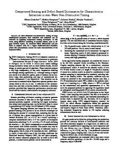
I. I NTRODUCTION Because of the advantages of large transmission bandwidth, low power consumption, and simple transceiver architecture, ultra wide band (UWB) technology has been widely utilized in many applications, such as UWB communications, medical imaging and wall penetrating radar. Particularly, due to the extremely short duration of UWB pulse (thus high time resolution), UWB pulse can be utilized for precise positioning and indoor navigation systems. However, it also brings the challenge of acquiring and detecting the ultra-short UWB pulses at the receiver side. Moreover, in many UWB systems, the need of acquiring a high resolution UWB pulse requires a 10GHz or even higher sampling rate at the receiver side. To meet such a demand, we propose to apply the theory of compressed sensing (CS) [1] [2] [3], which flourishes in recent years, since UWB signals are sparse in the time domain (the duty cycle of UWB signals is usually very small). The philosophy is to compress the received signal into a lowerdimensional space, thus reducing the required sampling rate, and then reconstruct the original UWB pulses. For applying CS, we face the following two difficulties: • How to efficiently compress the original received signal? • How to reconstruct UWB signals in a timely manner? We seek help from hardware implementations. For the former question, we use a bank of low sampling rate Analog-toDigital converters (ADCs) and microwave distributed amplifiers (DA) for compressing the original signal; for the latter problem, we consider filed programmable gate array (FPGA) implementation of signal reconstruction. The overall structure of our design is shown in Fig. 1: after a wide band antenna, received UWB pulses are amplified by low noise amplifier, divided into several channels by a wide-band power divider, and then fed into a bank of DAs and ADCs; the UWB pulses

Wide Band Power Divider

Distributed Amp

ADC

Distributed Amp

ADC

LNA

FPGA /DSP Distributed Amp

ADC

Distributed Amp

ADC

Fig. 1: Receiver structure

are mixed via the DAs and ADCs and then reconstructed by a FPGA. The remainder of the paper is organized as follows: the model of UWB signals, as well as basics about CS, is discussed in Section II; hardware based signal compressing and reconstruction are discussed in Sections III and IV, respectively; numerical results and conclusions are provided in Sections V and VI, respectively. II. UWB S IGNAL M ODEL AND C OMPRESSED S ENSING A. UWB Signal For a transmitted UWB pulse, the received signal in the time domain is given by x(t) =

L X

al p(t − tl ),

(1)

l=1

where L is the number of resolvable propagation paths, al is the amplitude gain coefficient along the l-th path, p(t) is the transmitted signal waveform and tl is the time delay of the l-th path. For simplicity of discussion, we ignore the noise in the received signal. Note that a Gaussian noise may incur substantial performance degradation. Bayesian compressed sensing and turbo signal reconstruction are used to alleviate the effect of noise in an accompanying paper [4]. B. Compressed Sensing In a general situation, denote the original signal by an mvector x and suppose that the sparsity (i.e. the number of nonzero elements in x), denoted by k, satisfies k ¿ m. Then, we can mix the signal in a linear manner, i.e. y = Ax,

(2)

2

The coefficients of gain cells can be either predefined or reconfigured to meet the requirements of measurement matrix. In this paper, these gain coefficients are random numbers conforming to the requirement of CS measurement matrix. Note that, in practice, the nonlinearity of gain cell in different frequency bands may introduce polynomial multiplication terms. However, under small signal model in our case, the nonlinear effect can be largely alleviated. For simplicity of discussion, we ignore the nonlinearity effect. •

Input T.L.

T. L.

Gain Cell

TL ..

T.L.

VCC

Terminal Resistance

Output TL ..

TL ..

T.L.

T.L.

Terminal Resistance

Fig. 2: Illustration of the inner structure of distributed amplifier where A is an n × m measurement matrix and y is the n-dimensional vector signal of measurements. If k is much smaller than m, we need much less observations to measure vector y, thus substantially reducing the required sampling rate. Fortunately, numerous algorithms for signal reconstruction in the theory of CS, such as Basis Pursuit (BP), Orthogonal Match Pursuit (OMP) and Stagewise Orthogonal Match Pursuit (STOMP), guarantee that the original signal x can be reconstructed from the observed signal y, provided that k is much smaller than m (sparsity assumption). This provides an approach to reduce the required number of samples for acquiring UWB pulses since UWB pulses are sparse in the time domain. III. S IGNAL C OMPRESSING VIA DA AND ADC In this section, we first briefly introduce DA and then discuss how to compress the original signal via DAs and ADCs. A. Distributed Amplifier DA, also called transversal filter, is a microwave circuit that has been invented for many decades. As shown in Fig. 2, a DA consists of multiple repeated taps, each containing a section of micro-strip input and output transmission lines, and the gain cell. This periodic architecture forms a special transmission line [6] [7]. The output of a DA at time t is given by y(t) =

m X

aj x(t − jτ ),

(3)

j=1

where m is the number of taps in a DA, {aj }j are attenuation coefficients of different gain cells, which can be set randomly, x is the input signal and τ is the fixed time delay of each section of transmission line. The DA is suitable for analog CS processing in the following three aspects: • The transmission line in DA supports UWB signal propagation with almost perfect impedance match. The characteristic impedance of transmission line changes very little over several GHz, thus, the waveform of the propagating UWB signal, S(t), is maintained. • The time delays, determined by the length of transmission line along which the signal propagates, can easily achieve time scale of 50ps, or less based on different substrates and technologies without changing the structure of DA [7].

B. Signal Compressing As shown in Fig. 1, the received signal is put into n DAs, which have different coefficients, and then sampled by n ADCs. On ignoring quantization noise, the output of the ith ADC is given by yi =

m X

aij xj ,

(4)

j=1

where xj = x(lTs − jτ ), Ts is the sampling period of ADCs and aij is the coefficient of the j-th gain cell of the i-th AD. Defining x = (x1 , ..., xm ) and y = (y1 , ..., yn ), we obtain the linear compressing equation in (2), where the measurement matrix is given by   a11 a12 · · · a1m  a21 a22 · · · a2m    A= . (5) .. ..  . ..  .. . . .  an1 an2 · · · anm IV. S IGNAL R ECONSTRUCTION VIA FPGA FPGA is an efficient approach of hardware implementation for signal reconstruction. Due to limited space, we consider only the implementation of OMP algorithm. A. Original OMP The procedure of OMP is given as follows: 1) Initialization: set residual error as r0 = y; set active set K0 = Φ; 2) For the t-th iteration, compute projection: ct = AT rt−1 .

(6)

Choose the index having the largest projection, i.e. λt = arg max |(ct )i | . t=1,...,n

(7)

Then insert index λt into the set Kt−1 to obtain Kt . Compute the solution xt = arg min ky − At xk, x

(8)

where At is obtained from the columns in A having indices in the set Kt . Then, update the residual vector r t = y − At x t ,

(9)

3) Check the residual vector: if krt k is smaller than a predetermined threshold, stop and output xt as the final result; otherwise, increase t by 1 and go back to Step 2.

3

B. Least Square Problem The key difficulty for implementing the OMP algorithm is the least square problem in (8), which is equivalent to solving the following problem: ¡ T ¢ At At xt = At y. (10) There could be plenty of approaches to solve the above equation, e.g. SVD, QR and Cholesky decomposition. In this paper, we adopt the Cholesky decomposition (the reason will be explained later), which decomposes the symmetric matrix ATt At into ATt At = Lt LTt ,

(11)

where Lt is a lower triangular matrix. The advantage of choosing Cholesky decomposition is that the matrix Lt can be updated incrementally and need not be completely recomputed in each iteration. To see this, we have ATt At µ T At−1 At−1 = hTt

ht g

Fig. 3: Hardware architecture in FPGA and x1 = r1 /Σ11 .

¶ ,

(12)

Clock 2: Get r2 from RAM; compute

¡ ¢T where hTt , g is the new column in matrix ATt At , compared with ATt−1 At−1 . It is easy to verify that

= =

r3 − a32 r2 r4 − a42 r2

and

L LT µt t Lt−1 = wtT

0 v

¶µ

LTt−1 0

wt v

¶ .

Lt−1 wt = ht , (14) √ and the scalar v = g. To avoid many operations of divisions and utilize pipelining, we modify the Cholesky decomposition to LDL decomposition, i.e. =

Lt Σt LTt ,

(15)

where Σt is a diagonal matrix and Lt is a lower triangular matrix having unit diagonal elements. The updates of Lt and Σt are similar to the above discussion. C. Pipelining When solving the linear equation with lower triangular matrix, we can using pipelining to accelerate the computation. Take a 4-dimensional equation for instance:       1 0 0 0 x1 y1  a21 1     0 0     x2   y2  (16)  a31 a32 1 0  Σ  x3  =  y3  . a41 a42 a43 1 x4 y4 The equation can be solved using the following pipelining: Clock 1: Get r1 = y1 from RAM; compute r2 r3

= =

y2 − a21 r1 y3 − a31 r1

r4

=

y4 − a41 r1 ,

x2 = r2 /Σ22 .

(13)

Obviously, we need only compute the new vector w by solving the following equation

ATt At

r3 r4

Clock 3: Get r3 from RAM; compute r4

=

r4 − a43 r3

and x3 = r3 /Σ33 . Clock 4: Get r4 from RAM; compute x4 = r4 /Σ44 . The corresponding hardware architecture is shown in Fig. 3. Notice that the basic arithmetic units are adders and multipliers. V. N UMERICAL R ESULTS In numerical simulations, a 500ps-duration first derivation Gaussian pulse is used as the transmitted signal. The indoor line-of-sight (LOS) propagation channel model (CM1) from the IEEE 802.15.4a working group in [5] is adopted for numerical simulations. Suppose that the resolution of recovered signal is 100ps, which is also the time delay of each tap in DA. The number of taps in DA is linearly increased while decreasing the sampling rate of the following ADCs. In addition, the number of DAs and ADCs determines the number of samples, which is directly associated with the quality of signal reconstruction. Recovery percentage is used to evaluate the system performance: kˆ x − xk , (17) δ =1− kxk

4

UWB pulses, FPGA is used for hardware implementation and the corresponding computational issues are discussed. R EFERENCES

Fig. 4: Recovery percentage with respect to different numbers of DAs and ADCs.

Fig. 5: Recovery percentage with respect to different numbers of DAs and ADCs when noise exists. ˆ is the estimate of the original signal. The recovery where x percentage is shown in Fig. 4 with respect to different numbers of DAs and ADCs. Four curves of recovery rate, representing designs using 250M samples per second (SPS), 500MSPS, 625MSPS and 1GSPS ADC, are displayed as the function of the number of DAs and ADCs. Basis Pursuit (BP) is used to recover the UWB signal with L1 -norm linear optimization. As seen from Fig. 4, there exists a tradeoff between the number of DAs (as well as ADCs) and the sampling rate of ADCs: if using slower speed ADCs, more DAs and ADCs are needed to achieve the same performance. Using our proposed design and measurement matrix, under the special pulse basis, we need only 8 DAs and ADCs with 500MSPS to achieve a recovery percentage of 97.8%. Simulation results with the sampling rate of 500SPS when noise exists are shown in Fig. 5. Gaussian noise is considered, whose signal-to-noise ratio (SNR) is labeled for different curves in Fig. 5. Obviously, the performance is substantially degraded, which motivates the study on signal reconstruction for noisy channels [4]. VI. C ONCLUSIONS In this paper, we have discussed the application of compressed sensing in UWB receivers to alleviate the problem of high sampling rate. Two fundamental problems, compressing and reconstruction, are considered. For linearly compressing the original signal, for the purpose of decreasing required sampling rate, a bank of DAs are used to construct a measurement matrix, followed by ADCs. For reconstructing the

[1] E. J. Cand`es, J. Romberg and T. Tao,“Robust uncertainty principles: Exact signal reconstruction from highly incomplete frequency information”, IEEE Trans. Inform. Theory, Vol. 52, no.2, pp. 489–509, Feb. 2006. [2] D. L. Donoho,“Compressed sensing”, IEEE Trans. Inform. Theory, Vol. 52, no.4, pp. 1289–1306, April 2006. [3] D. L. Donoho, M. Elad and V. Temlyakov,“Stable recovery of sparse overcomplete representations in the presence of noise”, IEEE Trans. Inform. Theory, Vol. 52, no.1, pp.6–18, Jan. 2006. [4] H. Li, D. Yang, G. D. Peterson and A. Fathy, “UWB acquision in locationing systems: Compressed sensing and Turbo signal reconstruction”, submitted to CISS 2009. [5] A. F. Molisch, “IEEE 802.15.4a channel model - Final report”, IEEE 2004 [Online]. [6] D. M. Pozar, Microwave Engineering, Wiley, 1998. [7] Y. Zhu, J. D. Zuegel, J. R. Marciante,and H. Wu, “A reconfigurable, multi-Gigahertz pulse shaping circuit based on distributed transversal filters ”, IEEE ISCAS, 2006.