Kalman Filtering for Compressed Sensing - CiteSeerX

Kalman Filtering for Compressed Sensing Dimitri Kanevsky1 , Avishy Carmi2,3 , Lior Horesh1 , Pini Gurfil2 , Bhuvana Ramabhadran1 , Tara N Sainath1 1 IBM T. J. Watson, Yorktown, NY 10598, USA 2 Technion - Israel Institute of Technology, Haifa 32000, Israel 3 Ariel University Center, Ariel 40700, Israel

Abstract – Compressed sensing is a new emerging field dealing with the reconstruction of a sparse or, more precisely, a compressed representation of a signal from a relatively small number of observations, typically less than the signal dimension. In our previous work we have shown how the Kalman filter can be naturally applied for obtaining an approximate Bayesian solution for the compressed sensing problem. The resulting algorithm, which was termed CSKF, relies on a pseudomeasurement technique for enforcing the sparseness constraint. Our approach raises two concerns which are addressed in this paper. The first one refers to the validity of our approximation technique. In this regard, we provide a rigorous treatment of the CSKF algorithm which is concluded with an upper bound on the discrepancy between the exact (in the Bayesian sense) and the approximate solutions. The second concern refers to the computational overhead associated with the CSKF in large scale settings. This problem is alleviated here using an efficient measurement update scheme based on Krylov subspace method.

in radiology, biomedical imaging and astronomy [3, 4]. Other applications consider model-reduction methods to enforce sparseness for preventing over-fitting and for reducing computational complexity and storage capacities. The reader is referred to the seminal work reported in [1] and [2] for an extensive overview of CS theory.

Keywords: Compressed sensing, Krylove subspace method

CS theory has drawn much attention to the convex relaxation methods. It has been shown that the convex l1 relaxation yields an exact solution to the recovery problem provided two conditions are met: 1) the signal is sufficiently sparse, and 2) the sensing matrix obeys the so-called restricted isometry property at a certain level. A complementary result guarantees high accuracy when dealing with noisy observations, yielding recovery ‘with overwhelming probability’. To put it informally, it is likely for the convex l1 relaxation to yield an exact solution provided that the involved quantities, the sparseness degree s, and the sensing matrix dimensions m × n maintain relation of the type s = O(m/ log(n/m)).

1

Kalman

filter,

Introduction

Recent studies have shown that sparse signals can be recovered accurately using less observations than what is considered necessary by the Nyquist/Shannon sampling principle; the emergent theory that brought this insight into being is known as compressed sensing (CS) [1, 2]. The essence of the new theory builds upon a new data acquisition formalism, in which compression plays a fundamental role. From a signal processing standpoint, one can think about a procedure in which signal recovery and compression are carried out simultaneously, thereby reducing the amount of required observations. Sparse, and more generally, compressible signals arise naturally in many fields of science and engineering. A typical example is the reconstruction of images from under-sampled Fourier data as encountered

The recovery of sparse signals is in general NPhard [1, 5]. State-of-the-art methods for addressing this optimization problem commonly utilize convex relaxations, non-convex local optimization and greedy search mechanisms. Convex relaxations are used in various methods such as LASSO [6], the Dantzig selector [7], basis pursuit and basis pursuit de-noising [8], and least angle regression [9]. Non-convex optimization approaches include Bayesian methodologies such as the relevance vector machine, otherwise known as sparse Bayesian learning [10], as well as stochastic search algorithms that are mainly based on Markov chain Monte Carlo techniques [11–14]. Notable greedy search algorithms are the matching pursuit (MP) [15], the orthogonal MP [16], and the orthogonal least squares [17].

Recently, a Bayesian CS approach has been introduced in [18]. As opposed to the conventional nonBayesian methods, the Bayesian CS has the advantage of providing the complete statistics of the estimate in the form of a posterior probability density function

(pdf). Adopting this approach, however, suffers from the fact that rarely one can obtain a closed-form expression of the posterior and therefore approximation methods should be utilized. In this paper we extend our previous work in [19] where we have presented the so-called CSKF which is a novel approximate Bayesian CS scheme based on the Kalman filter. There are two major issues which were left unanswered in [19] that are addressed inhere. The first one concerns the validity of the so-called pseudo-measurement approximation technique used by the CSKF to enforce the sparseness-promoting prior. The second issue is related to the excessive computational overhead associated with the Kalman filter update stage in large scale settings. Our endeavor in providing a proper answer to the first concern involves a unique type of sparseness-promoting prior, termed here semi-Gaussian owing to its Gaussian-like characteristics. We show how an approximate variant of this prior is, in fact, the probabilistic interpretation of the pseudomeasurement constraint. This in turn allows us to formulate an upper bound on the discrepancy between the exact and the approximate posterior pdfs based exclusively on the computed estimation error covariance. Finally, we provide a computational scheme that relies on Krylov subspace method for alleviating the workload associated with the CSKF measurement update stage which thereby renders it highly efficient in large scale CS settings.

2

Sparse Signal Recovery

This section, which is taken from [19], briefly overviews the main concepts underlying compressed sensing. Consider an Rn -valued random discrete-time process {xk }∞ k=1 that is sparse in some known orthonormal sparsity basis ψ ∈ Rn×n , that is zk = ψ T xk , s := #{supp(zk )} < n, where supp(zk ) and # denote the support of zk and the cardinality of a set, respectively (i.e., #{supp(zk )} denotes the number of nonzero elements of zk ). Assume that zk evolves according to zk+1 = Azk + wk , z0 ∼ N (µ0 , P0 ) (1) where A ∈ Rn×n is the state transition matrix and {wk }∞ k=1 is a zero-mean white Gaussian sequence with covariance Qk  0. Note that (1) does not necessarily imply a change in the support of the signal. For example, A can be a block-diagonal matrix decomposed of Ad and An corresponding to the statistically independent elements z d ∈ / supp(zk ) and z n ∈ supp(zk ) where the respective noise covariance sub-matrices satisfy Qd = 0 and Qn  0. The process xk is measured by the Rm -valued random process yk = Hxk + ζk = H 0 zk + ζk

(2)

where {ζk }∞ k=1 is a zero-mean white Gaussian sequence with covariance Rk  0, and H := H 0 ψ T ∈ Rm×n . Letting Yk := [y1 , . . . , yk ], our problem is defined as follows. We are interested in finding a Yk -measurable estimator, x ˆk , that is optimal in some sense. Often, the sought after estimator is the one that minimizes  the mean square error (MSE) E k xk − x ˆk k22 . It is well-known that if the linear system (1), (2) is observable then the solution to this problem can be obtained using the Kalman filter (KF). On the other hand, if the system is unobservable, then the regular KF algorithm is useless; if, for instance, A = In×n , then it may seem hopeless to reconstruct xk from an under-determined system in which m < n and rank(H) < n. Surprisingly, this problem may be circumvented by taking into account the fact that zk is sparse.

2.1

The Combinatorial Problem and Compressed Sensing

Refs. [1, 5] have shown that in the deterministic case (i. e., when z is a parameter vector), one can accurately recover z (and therefore also x, i.e., x = ψz) by solving the optimization problem min k zˆ k0 s.t.

k X i=1

k yi − H 0 zˆ k22 ≤ 

for a sufficiently small , where k v kp =

P

n j=1

(3) vjp

1/p

is the lp -norm of v, and the zero-norm, k v k0 , is defined as1 k v k0 := # {supp(v)}. Following a similar rationale, in the stochastic case the sought-after optimal estimator satisfies [2]   min k zˆk k0 s.t. Ezk |Yk k zk − zˆk k22 ≤  (4)

Unfortunately, the above optimization problems are NP-hard and cannot be solved efficiently. Recently, it has been shown that if the sensing matrix H 0 obeys a so-called restricted isometry property (RIP) then the solution of the combinatorial problem (3) can almost always be obtained by solving the constrained convex relaxation [1, 2] min k zˆ k1 s.t.

k X i=1

k yi − H 0 zˆ k22 ≤ 

(5)

This is a fundamental result in CS theory [1, 2]. The main idea is that the convex l1 minimization problem can be efficiently solved using a myriad of existing methods, such as LASSO [6], LARS [9], Basis pursuit [8], orthogonal matching pursuit [16] and relevance vector machine [10]. Other insights provided by CS are related to the construction of sensitivity matrices that satisfy the RIP. These underlying matrices are random 1 For 0 ≤ p < 1, k v k is not a norm; the common terminology p is zero norm for p = 0 and quasi-norm for 0 < p < 1.

by nature, which sheds a new light on the way observations should be sampled. For an extensive review of CS the reader is referred to [1, 2].

3

The CS-Embedded KF

The CSKF algorithm is aimed at solving a stochastic CS problem of the form   (6) min Ezk |Yk k zk − zˆk k22 s.t. k zˆk k1 ≤ 0 zˆk

It can be shown that for proper values of the tuning parameters 0 and , the solution of both (6) and the convex l1 relaxation of (4) coincide. The nonlinear inequality constraint in (6) is readily treated within the conventional KF framework using a so-called pseudomeasurement (PM) technique [19]. In practice this is carried out by recasting this constraint as ¯ k z k − 0 , 0=H

¯ k := sign(zk ) H

(7)

where sign(zk ) denotes a row vector consisting of the signs of the entries in zk . This formulation facilitates the implementation of the standard KF update equations which are provided in Algorithm 1 for the sake of completeness. Notice that this approach assumes that Algorithm 1 CSKF PM update stage 1

1: Set zˆ = zˆk|k and P

1

= Pk|k (the posterior mean and covariance at time k). 2: for τ = 1, 2, . . . , Nτ − 1 iterations do 3:

zˆτ +1 P τ +1

¯ τ = sign(ˆ H zτ )  ¯TH ¯τ PτH = I − ¯ τ ¯τT zˆτ Hτ P Hτ + σ 2   ¯TH ¯τ PτH = I − ¯ τ ¯τT Pτ Hτ P Hτ + σ 2 

(8a) (8b)

p(z | Yk ) = R

Bayesian Interpretation

The PM constraint (7) provides a convenient way for incorporating the nonlinear l1 inequality within the KF. Its tightness, and therefore the overall estimation accuracy, is controlled by both σ 2 and the total number of iterations Nτ per measurement update. In [19] we have mentioned that the tradeoff between the associated computational complexity and the obtained accuracy can be regulated by properly setting these two parameters. In this work we provide a supporting result to this argument. Specifically, we derive an upper bound on the estimation accuracy which alludes the relation with the PM variance σ 2 . In order to meet this end we shall restrict ourselves inhere to the conventional static

(9)

(10b)   where Pk = E (z − zˆk )(z − zˆk )T | Yk and zˆk = E [z | Yk ]. It can be easily shown that in this case zˆk is not only the minimum MSE estimator but also the maximum a posteriori (MAP) estimator, that is zˆk = arg max log p(z | Yk ) z

z

(8c)

0 is a random quantity, specifically a zero-mean Gaussian random variable with variance σ 2 .

p(yk | z)p(z | Yk−1 ) p(yk | z)p(z | Yk−1 )dz

where the likelihood p(yk | z) = pζk (yk − H 0 z). Because a Gaussian pdf is self-conjugate it readily follows that whenever the pdfs in the right-hand side of (9) are Gaussian the posterior can be described exclusively by its first two moments. These are given by the KF update equations
−1 [yk − H 0 zˆk−1 ] zˆk = zˆk−1 +Pk−1 H 0T H 0 Pk−1 H 0T + Rk (10a) h
−1 0 i 0 0T 0T H Pk−1 H + Rk H Pk−1 Pk = I − Pk−1 H

= arg min

4: end for 5: Set zˆk|k = zˆNτ and Pk|k = P Nτ .

3.1

linear model used in CS theory (i.e., Ak = In×n and Qk = 0n×n in (1)). Our derivations in this section, which are concluded with the formulation of an upper bound on the discrepancy between the exact and the estimated posterior pdfs, rely on the Bayesian formulation of the KF update stage. For that reason we take the time to revisit some well-established elementary results from estimation theory. Under the restrictions above, the posterior pdf of the random parameter vector z conditioned on Yk can be sequentially computed via the well-known Bayesian recursion

k X i=1

k yi − H 0 z k2Ri + k z − µ0 k2P0

(11)

where k a k2R := aT R−1 a. 3.1.1

Semi-Gaussian Priors

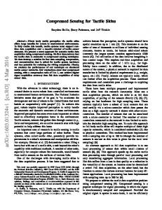
Compressed sensing was embedded in the framework of Bayesian estimation by utilizing sparsenesspromoting priors such as Laplace and Cauchy [18]. As opposed to the conventional CS methods, which provide a point estimate, the Bayesian approach yields the statistics p(z | Yk ). We have seen that the posterior pdf is entirely described by (10) in the linear Gaussian case. When resorting to non-Gaussian (sparsenesspromoting) priors, however, this recursion is strictly inadequate. Let us now consider a new type of sparsenesspromoting prior, which we will term semi-Gaussian   1 k z k21 (12) p(z) = c exp − 2 σ2 Compared with the Laplace distribution, the semiGaussian pdf concentrates greater portion of its mass in

the vicinity of the origin. This is illustrated in Fig. 1, in which the level maps are shown for Laplace, semiGaussian and Gaussian pdf’s in the 2-dimensional case.

100

100

90

90

80

80

70

70

60

60

50

50

40

40

30

30

20

20

10

10 10

20

30

40

50

60

70

80

90

100

10

(a) Laplace

20

30

40

50

60

70

80

90

100

(b) Semi-Gaussian

100 90 80 70 60 50 40 30 20

albeit varying, sensing matrices, (14) cannot be embedded straightforwardly. Nevertheless, its Gaussian approximation, in which the sensing matrix takes the ¯ := sign(ˆ form H zk ) (i.e., by substituting the estimator zˆk rather than z), can be easily processed via (10). ¯ a Yk -measurable quantity, This modification renders H as it depends on zˆk , which is a function of the entire observation set. The reader has probably realized by now that embedding the approximate semi-Gaussian prior within the Bayesian recursion (9) merely yields the PM stage described in Algorithm 1. Bearing in mind this, the unique formulation (14) allows us to assess the validity of the PM constraint (7) when enforcing the semiGaussian prior (12). Thus, the following theorem establish an upper bound on the discrepancy between the exact posterior, which relies on the semi-Gaussian prior (12), and the approximate posterior (i.e., the one that is computed by the CSKF) in terms of the CSKF estimation error covariance Pk .

10 10

20

30

40

50

60

70

80

90

100

(c) Gaussian Figure 1. Laplace, semi-Gaussian and Gaussian pdf ’s in the 2-dimensional case. Suppose for a moment that one embeds this prior within the Bayesian recursion (9) for promoting the sparseness of z. This in turn renders the closed form recursion (10) inadequate. This follows readily from the fact that the restrictions under which (10) are derived involve a purely-Gaussian prior and a likelihood pdf that is based on a deterministic sensing matrix H 0 ,   1 p(yk | z) ∝ exp − (yk − H 0 z)T Rk−1 (yk − H 0 z) 2 (13) Nevertheless, it turns out that the unique form (12) facilitates an approximate computation of the posterior p(z | Yk ) using the closed form recursion (10). As it is shown next, the approximate semi-Gaussian prior is closely related to the PM constraint (7) used by the CSKF. 3.1.2

Approximate Semi-Gaussian

The semi-Gaussian prior can be expressed based on the likelihood (13) using a sensing matrix similar to the ¯ := sign(z) and setting y = 0 one in (7). Thus, letting H in (13) yields  ¯ 2 1 (0 − Hz) p(z) = p(y = 0 | z) ∝ exp − 2 σ2

(14)

Although (14) resembles a Gaussian pdf its in fact a ¯ on z. As semi-Gaussian owing to the dependency of H the KF update stage (10) permits only deterministic,

Theorem 1. Let pˆ(z | Yk ) be the Gaussian posterior pdf obtained by using the approximate semi-Gaussian prior. Let also p(z | Yk ) be the posterior pdf obtained by using the exact semi-Gaussian prior (12). Then KL (ˆ p(z | Yk ) k p(z | Yk )) = o  n (15) O σ −2 max Tr(Pk ), Tr(Pk )1/2 where KL and Tr denote the Kullback-Leibler divergence and the matrix trace operator, respectively. The proof is provided in the Appendix.

3.2

Discussion

The fundamental observation conveyed by Theorem 1 is that the approximation error of the PM stage in Algorithm 1 is affected by both the prior variance σ 2 and the estimation error covariance Pk . Consequently, regulating these factors is beneficial in getting close to the exact CS solution in the Bayesian sense. This can be attained by either increasing σ or having a sufficiently small Pk . The former approach, however, might bring upon an adverse effect as the sparseness constraint is less restrictive in such cases. A prominent advantage of the bound (15) is that it involves quantities that are either known (σ 2 ) or computed (Pk ). Whereas σ is a predetermined tuning parameter, the estimation error covariance Pk , which is computed at every step, decreases rapidly as k → ∞ (in the sense that Pk − Pk+1  0). This fact readily follows upon recognizing that (10b) and (8c) trans−1 late into Pk−1 = Pk−1 + H 0T Rk−1 H 0 and (P τ +1 )−1 = τ −1 −2 ¯ T ¯ (P ) + σ H H by the matrix inversion lemma. Combining this observation with Theorem 1 explains why it is advantageous√ to perform Nτ consecutive updates of (8) using σ = Nτ σ 0 rather than a single update with σ 0 .

It should be clarified that Pk does not represent the exact estimation error covariance (i.e., the one which is based on the semi-Gaussian prior (12)). Nevertheless, as stated by Theorem 1, the trace of this matrix indicates the proximity of the obtained solution to the exact Bayesian one. An upper bound on the exact estimation error covariance can be obtained based on the result in [2] (Theorem 4.1). Thus, assuming z is at most ssparse and H 0 satisfies the RIP at the level δ3s +δ4s < 2, yields 2    p Tr E (z − zˆk )(z − zˆk )T | Yk ≤ c1 Tr(Rk ) + c2 e (16) where e denotes the reconstruction error in the noiseless case. For reasonable values of δ4s , the constants c1 and c2 in (16) are well behaved [2].

4

Computationally Efficient KF Update

When the state dimension n is large the computation of Pk becomes prohibitively expensive. In such cases we would like to avoid the explicit construction of large-scale dense matrices and their inverses. In addition, we recognize that exact computation of inverses is redundant in the course of defining a search direction within an optimization framework, especially when one is far from the solution. Both objectives can be achieved by employing a Krylov subspace method. It is a family of iterative methods that are extremely memory efficient, as only storage of the previous search direction and the local gradient requires for forming a new search direction. The Krylov subspace solver requires only implicit access to the matrices via matrix vector products [20]. Unlike the common situation when such approach is practiced directly, here the difficulty is that matrix inverses are nested within each other, as shown by Equation (10). For that reason we first recast the initial estimate of z from (10) as follows. We define an auxiliary function that computes the product of H 0 Pk−1 H 0T + Rk−1 by a vector v, which obeys the following property Hv = H 0 Pk−1 (H 0T v) + Rk−1 v

(17)

Notice, that the bracketed product of H 0 by v, abstain the need for explicit formulation of the largescale matrix H 0 Pk−1 H 0T . The inversion of the matrix H 0 Pk−1 H 0T + Rk−1 can now be obtained explicitly by solving the system Hv = yk − H 0 zˆk−1

(18)

In practice the above equation can be solved via the conjugate gradient method. Once (18) is solved it can be plugged back to yield the updated KF mean zˆk = zˆk−1 + Pk−1 H 0T v

(19)

In a similar manner, the covariance update stage is carried out as follows Pk = Pk−1 − Pk−1 H 0T M

(20)

where the columns mi of the matrix M ∈ Rm×n are obtained by solving Hmi = (H 0 Pk−1 )i ,

i = 1, . . . , n

(21)

where (H 0 Pk−1 )i denotes the ith column of H 0 Pk−1 .

5

Simulation Study

We demonstrate the previously described concepts using simple recovery examples taken from both [7] and [19]. In the first example we validate the relation conveyed by Theorem 1 which essentially implies that as the tuning parameter σ in (14) becomes larger the obtained approximate solution is closer to the exact one in the Bayesian sense. Thus, we would expect that increasing σ will result in smaller estimation errors. An adequate measure of sparse reconstruction accuracy, typically known as the ideal normalized estimation error, is given in [7]. This measure, which is defined as kz−

zˆk k22

/

n X i=1

min (z i )2 , Tr(R)/m




(22)

where z i denotes the ith element of z, quantifies the discrepancy between the attained estimation error and the ideal one which would have been obtained in the absence of measurement noise. In this example we consider a sensing matrix H ∈ R72×256 of which the entries are samples from a zeromean Gaussian distribution with variance 1/72. This type of matrix is known to satisfy the RIP with high probability for sufficiently sparse signals [2]. The sparseness degree of the actual parameter vector z is set as s = 10. The CSKF recovery errors in this case are shown for various values of σ in Fig. 2. This figure clearly demonstrates the idea underlying Theorem 1 as the attained estimation error (here after Nτ = 1000 iterations of the PM stage) reduces as σ increases. The two complementary panels in Fig. 3 illustrate the reconstruction performance of the CSKF when the parameter σ takes either of the two extremal values in Fig. 2, namely, σ = 100 and σ = 800. These rather qualitative figures visualize the estimation performance corresponding to the extremal values of the ideal normalized estimation error measure (as appears in Fig. 2). The performance of the computationally efficient CSKF, which embeds the Krylov solver method, is assessed in two distinct settings. These consist of sensing matrices of the size 512 × 1024 and 3072 × 6144 which are composed similarly to the abovementioned

Ideal normalized estimation error

500

0.8 0.6

400

0.4 0.2

300

0 200

−0.2 −0.4

100

−0.6 0 0

200

400 σ

600

−0.8 0

800

50

100

150 Index

200

250

(a) Ideal recovery error 443. σ = 100

Figure 2. The recovery errors attained for various values of the tuning parameter σ. The problem dimension in this case is H 0 ∈ R72×256 .

0.8 0.6

one. The accuracy of recovery is examined for various sparseness degrees s corresponding to the recovery index s/m log(n) which is derived from the relation m ≤ c(s log n) [2] (for some c > 0). This index essentially refers to the probability of recovery assuming the sensing matrix obeys the RIP up to a certain sparseness degree. As it was already pointed out in [2], as this measure increases an exact recovery becomes less probable. In all runs the Krylov solver method is employed as described in Section 4 using Matlab’s conjugate gradient (CG) function (assuming a tolerance of 10−3 and a maximal number of 200 iterations). The results of this example are given in Fig. 4 where the estimation errors of both the CSKF and its computationally efficient variant (CSKF+CG) are depicted for various recovery indices. From this figure it can be clearly seen that the Krylov solver method does not significantly affect the reconstruction accuracy of the CSKF. The prominent advantage of using the Krylov solver method is manifested in Fig. 5 where the timing data of both methods, the CSKF and its computational efficient variant, is shown for an increasing state dimension n. The sensing matrix used in this example is composed of samples from a zero-mean Gaussian distribution with variance 1/m with m = n/2 rows. In all runs, the sparseness degree s does not exceed n/6.

6

Conclusions

We have shown that the solution computed by the CSKF, which is a Kalman filtering-based approximate Bayesian compressed sensing algorithm, approaches the exact Bayesian solution as the PM tuning parameter σ increases. This result further justifies the iterative PM stage used by the CSKF (since as σ increases the sparseness constraint becomes less restrictive which thereby implies that more iterations are required).

0.4 0.2 0 −0.2 −0.4 −0.6 −0.8 0

50

100

150 Index

200

250

(b) Ideal recovery error 15. σ = 800 Figure 3. The actual (blue line) and reconstructed (red squares) signals for two extremal values of the parameter σ.

Embedding the Krylov solver method within the CSKF/Kalman filter measurement update stage dramatically reduces the computational overhead, in particular, when the state dimension is prohibitively large.

A

Proof of Theorem 1

The exact and the approximate posterior pdfs are given by   1 k z k21 p0 (z | Yk ) p(z | Yk ) = c exp − 2 σ2

(23a)

 ¯ 2 1 (Hz) pˆ(z | Yk ) = cˆ exp − p0 (z | Yk ) 2 σ2

(23b)

where c and cˆ denote the appropriate normalization constants, and p0 (z | Yk ) stands for the Gaussian posterior excluding the prior. Now, explicitly writing the

300

2 CSKF CSKF+CG

CSKF CSKF+CG 1.5

250 Time (Sec)

Ideal normalized estimation error

350

200 150 100

1

0.5

50 0 0

0.2

0.4 0.6 Recovery index

0.8

0

1

(a) 512 × 1024

500

1000 1500 State dimension n

2000

Figure 5. Computational load of the CSKF with and without the Krylov solver method.

Ideal normalized estimation error

70 60

CSKF CSKF+CG

gives KL (ˆ p(z | Yk ) k p(z | Yk ))  2  1 ˆ¯ 1 Hz | Yk = ≤ log(ˆ c/c) + 2 Eˆ k z k21 | Yk − 2 E 2σ 2σ  1 ˆ 1 2 log(ˆ c/c) + 2 E k z k1 | Yk − 2 k zˆk k21 (25) 2σ 2σ Further letting δz := z − zˆk , Eq. (25) yields

50 40 30 20 10 0

0.2

0.4 0.6 Recovery index

0.8

1

(b) 3072 × 6144 Figure 4. The estimation errors of the CSKF with and without the Krylov solver method for various recovery indices. Showing the performance for two problem dimensions, 512 × 1024 and 3072 × 6144.

KL divergence between these two pdfs yields

KL (ˆ p(z | Yk ) k p(z | Yk )) Z pˆ(z | Yk ) = pˆ(z | Yk ) log dz p(z | Yk ) Z   1 ¯ 2 dz pˆ(z | Yk ) k z k21 −(Hz) = log(ˆ c/c) + 2 2σ    1 1 ˆ ¯ 2 | Yk = log(ˆ c/c) + 2 E k z k21 | Yk − 2 Eˆ (Hz) 2σ 2σ (24)

KL (ˆ p(z | Yk ) k p(z | Yk ))  1 1 ˆ ≤ log(ˆ c/c) + 2 E k z k21 | Yk − 2 k zˆk k21 2σ 2σ i 1 1 ˆh 2 ≤ log(ˆ c/c)+ 2 E (k zˆk k1 + k δz k1 ) | Yk − 2 k zˆk k21 2σ 2σ  1 ˆ 1 ˆ = log(ˆ c/c)+ 2 E [k δz k1 | Yk ] k zˆk k1 + 2 E k δz k21 | Yk σ 2σ (26) owing to √ the triangle inequality. Recalling that k δz k1 ≤ n k δz k2 we may then write KL (ˆ p(z | Yk ) k p(z | Yk )) √   n nˆ [k δz k2 | Yk ] k zˆk k1 + 2 Eˆ k δz k22 | Yk ≤ log(ˆ c/c)+ 2 E σ 2σ √ 1/2 n ˆ 2 ≤ log(ˆ c/c) + 2 E k δz k2 | Yk k zˆk k1 σ  n ˆ k δz k22 | Yk (27) + 2E 2σ where the 2nd line in (27) is due to the Jensen inequality. Recognizing that   ˆ k δz k22 | Yk E    ˆ (z − zˆk )(z − zˆk )T | Yk = Tr(Pk ) (28) = Tr E

Eq. (27) can be written as ˆ | Yk ] denotes the expectation operator with where E[· respect to pˆ(z | Yk ). Applying the Jensen inequality ¯ zˆk =k zˆk k1 , zˆk = E[z ˆ | Yk ], while recalling that H

KL (ˆ p(z | Yk ) k p(z | Yk )) o  n (29) ≤ log(ˆ c/c) + O σ −2 max Tr(Pk ), Tr(Pk )1/2

At this point the theorem immediately follows owing to the inequality log(ˆ c/c) ≤ 0. In order to show this we ¯ 2 owing to the fact that the first note that k z k21 ≥ (Hz) left hand expression consists of summation of positive terms whereas the same terms on the right side of the equation have either positive or negative signs. This further implies

[8] S. S. Chen, D. L. Donoho, and M. A. Saunders, “Atomic decomposition by basis pursuit,” SIAM Journal of Scientific Computing, vol. 20, no. 1, pp. 33 – 61, 1998.

¯ 2 =⇒ − k z k21 ≤ −(Hz)    ¯ 2 1 k z k21 1 (Hz) exp − ≤ exp − =⇒ 2 σ2 2 σ2   Z 1 k z k21 p0 (z | Yk )dz exp − 2 σ2  Z ¯ 2 1 (Hz) p0 (z | Yk )dz =⇒ ≤ exp − 2 σ2 Z   −1 1 k z k21 0 exp − p (z | Y )dz k 2 σ2 −1 Z  ¯ 2 1 (Hz) 0 p (z | Yk )dz =⇒ c ≥ cˆ ≥ exp − 2 σ2 (30)

[10] M. E. Tipping, “Sparse Bayesian learning and the relevance vector machine,” Journal of Machine Learning Research, vol. 1, pp. 211 – 244, 2001.

QED.

References [1] E. J. Candes, J. Romberg, and T. Tao, “Robust uncertainty principles: Exact signal reconstruction from highly incomplete frequency information,” IEEE Transactions on Information Theory, vol. 52, pp. 489–509, 2006.

[9] B. Efron, T. Hastie, I. Johnstone, and R. Tibshirani, “Least angle regression,” Annals of Statistics, vol. 32, no. 2, pp. 407 – 499, 2004.

[11] R. E. McCulloch and E. I. George, “Approaches for Bayesian variable selection,” Statistica Sinica, vol. 7, pp. 339 – 374, 1997. [12] J. Geweke, Bayesian Statistics 5, chapter Variable selection and model comparison in regression, Oxford University Press, 1996. [13] B. A. Olshausen and K. Millman, “Learning sparse codes with a mixture-of-Gaussians prior,” Advances in Neural Information Processing Systems (NIPS), pp. 841 – 847, 2000. [14] S. J. Godsil and P. j. Wolfe, “Bayesian modelling of time-frequency coefficients for audio signal enhancement,” Advances in Neural Information Processing Systems (NIPS), 2003. [15] S. Mallat and Z. Zhang, “Matching pursuits with time-frequency dictionaries,” IEEE Transactions on Signal Processing, vol. 4, pp. 3397 – 3415, 1993.

[2] E. J. Candes, “Compressive sampling,” Madrid, Spain, 2006, European Mathematical Society, Proceedings of the International Congress of Mathematicians.

[16] Y. C. Pati, R. Rezifar, and P. S. Krishnaprasad, “Orthogonal matching pursuit: recursive function approximation with applications to wavelet decomposition,” 27th Asilomar Conf. on Signals, Systems and Comput., 1993.

[3] M. Lustig, D. Donoho, and J. M. Pauly, “Sparse MRI: The application of compressed sensing for rapid MR imaging,” Magnetic Resonance in Medicine, vol. 58, pp. 1182–1195, 2007.

[17] S. Chen, S. A. Billings, and W. Luo, “Orthogonal least squares methods and their application to non-linear system identification,” International Journal of Control, vol. 50, pp. 1873 – 1896, 1989.

[4] U. Gamper, P. Boesiger, and S. Kozerke, “Compressed sensing in dynamic MRI,” Magnetic Resonance in Medicine, vol. 59, pp. 365–373, 2008.

[18] S. Ji, Y. Xue, and L. Carin, “Bayesian compressive sensing,” IEEE Transactions on Signal Processing, vol. 56, pp. 2346 – 2356, June 2008.

[5] R. Chartrand, “Exact reconstruction of sparse signals via nonconvex minimization,” IEEE Signal Processing Letters, vol. 14, pp. 707–710, 2007.

[19] A. Carmi, P. Gurfil, and D. Kanevsky, “Methods for sparse signal recovery using kalman filtering with embedded pseudo-measurement norms and quasi-norms,” IEEE Transactions on Signal Processing, In print.

[6] R. Tibshirani, “Regression shrinkage and selection via the LASSO,” Journal of the Royal Statistical Society. Series B (Methodological), vol. 58, no. 1, pp. 267–288, 1996. [7] E. Candes and T. Tao, “The Dantzig selector: statistical estimation when p is much larger than n,” Annals of Statistics, vol. 35, pp. 2313–2351, 2007.

[20] L. Horesh, M. Schweiger, S.R. Arridge, and D.S. Holder, “Novel large-scale non-linear 3d reconstruction algorithms for electrical impedance tomography of the human head,” IFMBE, vol. 14, pp. 3862–3865, 2007.