Keywords: Color, Compression, HVS, Opponent Space, Wavelet ..... on the widely accepted theory of three neural pathways that process the color information.
Compression of color images with wavelets under consideration of the HVS Marcus J. Nadenau and Julien Reichel Signal Processing Laboratory, Swiss Federal Institute of Technology, Switzerland
ABSTRACT
In this paper we present a new wavelet-based coding scheme for the compression of color images at compression ratios up to 100:1. It is originally based on the LZC algorithm of Taubman. The main point of discussion in this paper is the color space used and the combination of a coding scheme with a model of human color vision. We describe two approaches: one is based on the pattern-color separable opponent space described by Poirson-Wandell; the other is based on the Y C C -space that is often used for compression. In this article we show the results of some psychovisual experiments we did to re ne the model of the opponent space concerning its color contrast sensitivity function. These are necessary to use it for image compression. They consist of color matching experiments performed on a calibrated computer display. We discuss this particular opponent space concerning its delity of prediction for human perception and its characteristics in terms of compressibility. Finally we compare the quality of the coded images of our approach to Standard JPEG, DCTune2.0 and the SPIHT coding scheme. We demonstrate that our coder outperforms these three coders in terms of visual quality. Keywords: Color, Compression, HVS, Opponent Space, Wavelet b
r
1. INTRODUCTION
There are many di�erent e�ects of the human visual system that can be considered separately: contrast sensitivity function (CSF), contrast-, frequency- or even entropy-masking. But the common factor is the color space in which the image is represented. Although this point is crucial, it is often treated in an inadequate way. This was our motivation to investigate the relationship between color space and contrast sensitivity function in the context of image compression in more detail. We chose a wavelet-based coding scheme because it o�ers the advantage over DCT schemes to provide spatial and frequency information at the same time, which corresponds to the human visual system (HVS) where both are used. There has been less research work done concerning color perception than for luminance perception. Mullen1 published color contrast sensitivity functions measured with combinations of mono-chromatic lasers, Rajala2 did measurements by de ning the contrast in La� b�, but not in the supra-threshold region of contrasts. Poirson and Wandell3 presented an interesting opponent color space that is based on a linear transformation. We decided to base our approach on this color space, because its feature of separability between color and pattern perception is useful for compression. We will see that it is necessary to have a color space that allows a good prediction of the human visual perception, but at the same time it should have good compressibility characteristics to be used for compression. It is di�cult to match both constrains at the same time. The paper is organized as follows: In section 2 we describe our wavelet-based coding scheme, section 3 explains the motivations to chose the particular used color space, section 4 describes our psycho-visual experiments to evaluate the color contrast sensitivity function, section 5 discusses the characteristics of this opponent color space and section 6 shows the results of the compression quality comparison.
2.1. General structure
2. THE CODING SCHEME
Our wavelet coder is derived from the layered zero coding (LZC) proposed by Taubman.4 Extended to application on color images we incorporated the human vision model. The color input image is decomposed by a wavelet decomposition using the bi-orthogonal Daubechies (9,7)- lter.5 Each color channel is treated separately. Fig. 1 shows the resulting structure for a three level decomposition. The wavelet coe�cients may be indicated with w . i
The coe�cient w can be located in any subband of any color channel. First, we determine the maximal coe�cient value of all subbands in all color channels w and normalize all coe�cients by this value to get a coe�cient range between (,1; 1). We can express the normalized coe�cients in a binary notation as: i
M
with w = maxkw k + 1 (1) w = ww = �0:b1b2 b3 b4 b5 b6 ::: Here the most signi cant bit (MSB) is b1 . The MSB of all coe�cients form layer L1 . All b2 form layer L2 and i
n i
M
M
i
i
so forth. In the zero layer coder, coding goes from the most signi cant layer to the less signi cant layers. For an implementation of integer based lters the normalization step can be also replaced by a modi ed thresholding comparison, which allows then lossless coding. 3
i=0 k=1 n c = first wi in scanning order
2 1 4
Y
Is c already coded as significant ?
Send bk(c)
N
bk(c)==1 ?
Refinement-Mode Y
N
Send SIG Send +/-
Send NO-SIG
Once through scan of all subbands ? Y k = k + 1; i = 0 to decrease the threshold
N i=i+1 n to get next wi corresponding to scanning order
C
Until bit-rate reached
Until bit-rate reached
Structure of 3 level wavelet decomposition. There is one plane per each color channel. The shaded pixels with the numbers indicate the scanning order between color channels, the arrow the zig-zag scan. The dark squares mark the context for the coe�cient to be coded (C). Right: Nassi-Schneiderman diagram of the basic coding algorithm. Figure 1. Left:
Fig.1 shows the three decomposition planes, each representing one color channel. The coding scan starts in the upper left corner with the rst subband and scans than as marked by numbers the three color planes at the same position. Then it continues with the next coe�cient in the rst subband in the rst plane. Once the rst subband is nished the scan continues with the next in the zig-zag order. Let k indicate the bit layer that is processed, starting with k = 1. If b of the actual coe�cient equals one, the coe�cient is classi ed as signi cant. As information the coder encodes: signi cant and the sign bit of the coe�cient. Once a coe�cient is classi ed as signi cant it will be re ned with the next scanning path. That means the bits b are transmitted. On the encoder and decoder side is kept track about the status of signi cant and not signi cant. The symbols are encoded by the JBIG QM-entropy coder,6 a QM-coder where the possible probability values are grouped into 113 xed states. Therefore the arithmetic coding can be performed by lookup operations. To achieve a good probability adaptation a context coding is used, built by the signi cant/insigni cant status of the neighbor coe�cients and the parent coe�cient. In the re nement mode no context information is used. The context distinguishes between 128 di�erent contexts. We determine the context of the status of 6 neighbor coe�cients and one parent coe�cient. The left side of Fig. 1 shows the coe�cients that are considered for the context as dark shaded squares. We use a separate context for the lowband, because of its di�erent coe�cient distribution. We also investigated di�erent constellations of contexts, such as larger or geometrically adapted (i.e. diagonal shape for subband with diagonal frequencies and so on) contexts; the coding performance was not signi cantly improved. k
k
2.2. Implementation of the HVS
The CSF of the human visual system can be exploited to optimize the quantization of the wavelet coe�cients. As the encoding scheme is progressive, we implemented in an earlier version the CSF in an adaptive manner. The
scheme would rst achieve a visually lossless quantization for large viewing distance, to change then continuesly in a prede ned manner the CSF-quantization to smaller and smaller viewing distances. It nally turned out that applying a xed HVS pre- and post- ltering for a viewing distance of 20 cm, does similar for qualities close to visually lossless. Another reason why we decided to apply here a xed ltering is the reduced complexity of the encoder. One way to implement a frequency weighting would be to take the mean value of the corresponding frequency range as weighting factor for a subband; the implementation realized in our adaptive CSF approach. In our current scheme we implemented the CSF curve by a FIR lter operation applied to the subbands. To keep the computational task low we constrain the ltering to separable lters that are applied in horizontal and vertical direction. This allows us to have di�erent lter function depending on the subband orientation. By applying the lter after the decomposition into subbands we can also apply other contrast computations before the HVS- ltering. Fig.2 visualizes how the CSF curve is linked to the frequency ranges of the subbands. The left gure shows the lterbank for the wavelet decomposition simpli ed to the one dimensional case. Each output signal contains a certain frequency range, where f indicates the original sampling frequency of the image. On the right side we see the corresponding subparts of the CSF, marked by the bars under the plot. The transfer function of the low- and high-pass lter are G(z ) respectively H (z ). Both contain the downsampling by factor 2 that maps the band-limited decomposition output signals to the base band, so that its normalized frequency f ranges for all outputs from 0 to 0:5. The HVS lters are assigned to the transfer functions A(z ); B (z ) and C (z ). The input signal of each of these lters is band-limited. Therefore these lters are low-pass lters with the transfer functions that represents the subparts of the CSF mapped to the normalized frequency range between 0 and f ( ) , where b�[L; H ] stand for low or high-pass lter, i = 1 : : : N indicate the decomposition level and N the number of decomposition levels. s
n
bi n
Input-Signal
LowPass
G(z)
HighPass
1
H(z)
Level 1
0.8
LowPass
G(z)
H(z)
HighPass
Level 2
Sensibility
0.6
High-Pass frequency range
0.4
Low-Pass frequency range 0.2
0... 1fs 8 (L2) 0... 1fn 2
A(z)
1 f ... 1 f 8s 4 s (H2) 0... 1fn 2
B(z)
1 f ... 1 f 4s 2 s (L1)
0... 1fn 2
Decomposition output-signals
C(z)
HVS Pre-Filtering
0.1
1
0.5fs
10 0
(L1)
0.1
(L1)
0.5 fn
Spatial Frequency in cyc/deg 0
(L2)
0.1
(H1)
A
(L2)
0.5 fn
(H2)
(H1)
0.5 fn
C
(H2)
0.5 fn
B
Left: It shows for the 1D-case the decomposition of the input signal by the wavelet- lterbank. At each output signal the corresponding frequency band is expressed by the input signal sampling frequency f and the normalized frequency f ( ) . Where b�[L; H ] stand for low- and high-pass and i for the decomposition level. The lters A : : : C represent the HVS lters. Right: The gure shows an example for a CSF to be incorporated in the coder. Parts of the CSF, covering just a subrange of spatial frequency are applied to the subbands. Figure 2.
s
bi n
For the two dimensional wavelet decomposition we get the LL-subband after ltering in horizontal and vertical direction with G(z ) (low-pass), the subbands containing the horizontal (HL) and vertical (LH) details by ltering with G(z ) and H (z ) (high-pass) once in horizontal once in vertical direction. For the diagonal details we apply H (z )
in both directions. The one dimensional HVS- lter function is given by (
,( +1) ) b = L with f � [, 1 : : : 1 ]; i = 1 : : : N T (f ) = W (jf jf 2 2 2 W ((1 + 2jf j)f 2,( +1) ) b = H n
bi
i
s
n
n
and extended to the 2D case by
(2)
n
i
s
8 TLi (fnh ) � TLi (fnv ) > > > < h v
b = LL T ( f ) � T ( f ) b = LH T (f ; f ) = > T (f ) � T (f ) b = HL > > : T (f ) � T (f ) b = HH: h n
bi
Li
v n
Hi
n
Hi
h n
Li
v n
Hi
h n
Hi
n
(3)
v n
Here b indicates the frequency band (subband for 2D), i the decomposition level and W (f ) the initial CSF function, as shown on the right hand side of Fig.2. The function W (f ) is assumed to be modeled by Eq.9. If a speci c CSF were measured for diagonal orientation, the goal of the lter design would be to separate this transfer function into a horizontal and vertical lter operation. In our case we do not have separate data. Therefore we use the CSF given for horizontal oriented patterns and apply it in both directions. Next, we derive the coe�cients for a FIR lter implementation by a Fourier series. We suppose T (f ) being zero symmetric and get its approximation by Eq.4 bi
n
X T^ (f ) = c0 + 2 c cos(kf ) L
bi
n
k
=
n
k=1
Z
1 2 0
2T (f )df + 2 bi
n
Z L X
[2
n
k=1
1 2 0
T (f )cos(kf )df ] cos(kf ): bi
n
n
n
n
(4)
The lter kernel is then [c ; : : : ; c1 ; c0 ; c1 ; : : : ; c ], where the lter length is 2S + 1. At the decoder side we perform the inverse lter operation. Its coe�cients can be similarly computed. The choice of the lter length depends on the desired analysis/synthesis (applying the ltering and inverse ltering in series) error. To keep it in a reasonable range a lter length in the order of S = 5 is su�cient. S
S
2.3. Contrast computation
For grayscale images exist several de nitions of contrast, i.e. the Michelson contrast. But for color it is di�cult to de ne something like a color contrast. However, any kind of contrast in a complex image or in a simple test pattern is relative to the surrounding background color. This background color is an average value over a region that depends on the viewed spatial frequency. For human perception the product of the radius of this region and the observed spatial frequency stays approximately constant. In the case of a wavelet decomposition the mean spatial frequency doubles from one to the next decomposition layer and the size of region is half the size. This corresponds well and motivates to consider the values of the LL band, containing the approximated pixel values at this decomposition layer, as representation of the mean background. A possible implementation is the division of the detail coe�cients by the corresponding value of the LL-subband to compute a contrast. The implementation of this has the disadvantage that the used LL-subband coe�cients at the decoder side are quantized and introduce a non-linear distortion that is di�cult to predict. Experiments with an implementation of the Michelson contrast for grayscale images did not show a signi cant improvement.
3.1. Standardized Color Spaces
3. COLOR SPACES
In the framework of color image compression the Y C C space is common. Its color space de nitions stem from the development of color television. Later on they were applied to other video applications like MPEG. From RGB to Y C C can be converted by a linear transformation. Although luminance-chrominance coordinates like the Y C C are convenient to use, they su�er from an important drawback: the perceived color change produced by a xed small change of the color coordinates is quite non-uniform (Mac-Adams ellipses). b
b
r
r
b
r
This drawback is largely addressed in CIELu�v� and CIELa� b� . These are intended to be perceptionally uniform spaces. The CIELu�v� and CIELa� b� coordinates express a color always as a di�erence to a reference color, i.e. the reference white of the displaying media. Unlike the Y in Y C C , the luminance is based on the CIE1976 lightness de nition, which is a non-linear function. This non-linearity compensates the non-linear contrast perception. The chrominance coordinates for CIELu�v� and CIELa� b� are similarly de ned by a non-linear transformation. These color spaces are designed to compare large uniform color patches (spatial frequency zero). This does not apply to natural imagery. Therefore we need a coordinate system that considers as well the dependency of spatial frequency. b
r
3.2. Pattern-Color Separable Opponent Color Space
The idea of the opponent color space is to model the color perception corresponding to the processing in the human brain. It is based on the widely accepted theory of three neural pathways that process the color information. The goal is to separate the property of color perception from its functional relation to the spatial frequency. This color-separable was designed by Poirson and Wandell,3,7 by nding the linear transformation that ts best the color-separable model. They represented colors in the cone contrast space, where each color is given by the color contrast de ned as � � � � �L ; �M ; �S = L , L ; M , M ; S , S ; (5) s =
L
M
S
B
L
B
M
B
B
B
S
B
where L, M, S stand for the long-,medium- and short wavelength cone fundamentals. Poirson-Wandell used the sensitivity description of Smith-Pokorny8 and peak normalized it to 1. The screen background for theirs experiments was de ned by (L ; M ; S ) and set in CIE 1931 Yxy coordinates to (49:8cd=m2; 0:27; 0:3) . The de nition of the Smith-Pokorny functions9 (SPF) is based on the CIE1951 XYZ coordinates. In the following we reference the peak normalized version of SPF as LMS. The transformation is given by B
B
B
2
3T
0:15514 0:54312 ,0:03286 [L; M; S ] = [X51 ; Y51 ; Z51 ] 4,0:15514 0:45684 0:03286 5 : 0 0 0:01608
(6)
Let us assume that our visual system represents the image as a neural image. The magnitude of the values of this image represent the perceived color contrast. Following the hypothesis of pattern-color separability, we assume that the values of this neural image o can be expressed by applying a separable matrix T = D C to the cone contrast vector s f
o
=T s=D f
f
:
Cs
f
(7)
The matrix C incorporates the color sensitivity for spatial frequency of zero cycles per degree (cpd) and the diagonal matrix D describes the sensitivity over spatial frequency. f
4. PSYCHO-VISUAL TESTS 4.1. Motivation for experiments
There are two di�erent types of psycho-visual experiments that can be performed to evaluate the matrices C and D : threshold detection experiments and color matching experiments. For the threshold test the color di�erence between the maximum and minimum intensity of the grating is decreased down to a level where it cannot be distinguished from the pattern surrounding background. In the second case a uniform color pattern and a color grating is displayed; the observer is asked to match the contrast of the uniform patch to the contrast of the same color in the color grating. Both methods evaluate the contrast sensitivity; the fundamental di�erence is that the threshold method determines the absolute threshold and the color matching method determines the relative behavior in the supra-threshold region. The absolute threshold value has the advantage that we can derive an importance weighting between the di�erent channels. The usually used color quantization of 8 bits per channel is producing well visible color di�erences, when only the in uence of the CSF is considered. In natural images this is hidden by masking e�ects. That means usually the computer graphics are operating, regarding the CSF, all the time in the supra-threshold region. Therefore it is necessary to do an interpolation from the measured data up to the supra-threshold region that is of interest for f
normal applications. To keep the introduced uncertainty of the model small we decided to go with the color matching model, where the sensitivity data is directly for the desired contrast region. Poison-Wandell3 present the results of such a matching experiment and the corresponding matrices C and D . Unfortunately the spatial frequency range is limited to maximal 8 cpd and the variation between the two observers is relatively big. This is also valid for the threshold experiment in.7 Even when Lai10 did additional experiments to apply the constant cycle opponent space7 to a quality measurement system, still the disadvantage of operating below the interesting contrast range is kept. Therefore we did additional experiments for the opponent space derived by color matching. f
4.2. Screen setup and test pattern
We displayed the test pattern for the evaluation of the CSF on a calibrated 21" screen, with Trinitron tube and an average pitch of 0:25 mm running in the resolution 1200 � 1600 pixels. To calibrate the display we measured the spectrum of the three tube phosphors with a spectrometer and determined the gamma curve. To maintain the calibration we did before each psycho-visual test a measurement with an XRite-DTP 92 colorimeter to reduce the daily uctuation caused by temperature, duration of on-time and so forth. This way we are able to display a desired CIE XYZ color on the screen. The color variations along the spatial location on the display were not compensated in our setup; however, we judged them to be in an acceptable range. The pitch varies slightly from the center to the border of the display, which reduces the maximal displayable spatial frequency by factor 2. So that at least 4 logical points should be present per pattern period. The color quantization of our equipment allows a 8-bit quantization per each color gun. There is not an optimal test pattern design criterion for all purposes; we compromised between pattern eld size, number of cycles, background, visual viewing angle, viewing distance and so forth. It can be observed that a higher number of cycles in the test pattern increases the contrast sensitivity. The minimal number of cycles that should be used is around 6 to 14 cycles.11,12 Some experiments were performed on rectangular test stimuli others are based on circular shape stimuli. Using a windowed circle shape pattern o�ers the advantage that there is no clear border to the test pattern. Howell11 determines a critical size for the rectangular test pattern beyond which the detection threshold did not vary any more. The critical size can be de ned as being 10 to 20 times the period length of the spatial frequency signal. This is valid for frequencies higher than 0.5 cpd. For lower frequencies the critical size is smaller. Takahashi shows13 that the stimulus size is not of importance as long as the contrast is above 0.1. For lower contrasts an increase of apparent contrast with bigger stimulus size is observed. A matched background (a background of the same mean luminance as the test pattern) increases the sensitivity compared to a surrounding dark background. The decision between sinusoidal or square-wave test pattern is mostly driven by the practical constraint of color quantization. To achieve a smooth color variation, necessary for sinusoidal pattern, more than 8bits of quantization are needed. The viewing distance does not seem to have any intrinsic e�ect on the contrast sensitivity; when possible it should be chosen rather natural (50-80cm). Based on the above, we decided to do the tests with a windowed circle shape pattern with a square-wave grating in horizontal direction. The most urgent constant is the minimal number of 6 cycles for the 0.5 cpd pattern, which results in a 12 degree test pattern. By choosing a diameter of 15 cm the viewing distance is given to 71.75 cm. Another constraint is that the highest spatial frequency pattern should be sampled with at least 4 pixels per period, caused by the pitch uctuation. We show the pattern on the screen in front of the mean luminance background. The screen itself is viewed binocular through a non-re ecting black cardboard tube that keeps the viewing distance xed and avoids undesired in uence of surrounding light.
4.3. Matching experiment and psycho-metric function tting
We display two circle shaped patches at the same time on the screen. On the left side the striped pattern with the horizontal grating, containing two colors. On the right side the uniform patch. The uniform patch is faded in and out to background color. The observer has to decide whether the contrast of the uniform patch is weaker or stronger than the corresponding color in the striped pattern. The observer has 2.5 seconds for his decision, otherwise the system blends automatically over to the next patch. We test each principal color axis of the opponent space in separate experiments for the spatial frequencies 0, 0:5, 0:7, 1, 2, 4, 8, 12:5 cpd. The rst series is composed of bluish black and white pattern, where the bluish black is matched; the second is composed of pink and green, where the pink is matched and the last series shows yellow-green
and violet color, where the violet is matched. The contrast of the striped pattern stays constant, while the contrast of the uniform patch is varied along the opponent axis from one to the next patch. The observers decision does not in uence the contrast of the next displayed patch. In a pre-selection phase of 20 matches the nal matching contrast is roughly estimated. Then another 60 tests around this pre-estimated contrast are performed. We compute the probability p (C ) that the uniform patch appears with a weaker contrast than the corresponding color in the pattern. It is de ned in Eq.8. The counters N ; N ; N are incremented corresponding to the answer of the observer: weaker, stronger, no answer. The relative contrast C is de ned in Eq.8, where o is the matching color of the patch and o the color in the grating, both given as opponent value. The opponent values o and o are scalars, because we use only test pattern with colors along the principal axis of opponent space. C (8) p (C ) = NN ++N0:5+NN p^ (C ) = e,( �r ) C = oo The psychometric function p^ (C ) is tted to the experimental data by minimizing the least mean square error, as shown on the left-hand side of Fig.3. The matching contrast C0 5 is the C for which p^ (C ) becomes 0:5. In the middle of Fig.3 we see the result of all these ttings for one observer and all three color channels. Finally we t our S
r
w
s
n
r
P
G
P
w
P
s
r
s
n
r
s
G
w
n
r
Fitting of psychometric function
0.6 0.5 0.4 0.3 0.2 0.1 0.4
0.5
0.6
Rel. Contrast Cr
0.7
s
0.8
1 0.9 0.8 0.7 0.6 0.5 0.4 0.3
0.2
r
CSF Combined Fitting Result
Relative contrast sensitivity
Relative contrast sensitivity
Probability ps(Cr )
C0.5
0.7
0.3
r
Observer MN
0.9 0.8
r
l
:
1
G
1 0.9 0.8 0.7 0.6 0.5 0.4 0.3 0.2
Luminance Red/Green Blue/Yellow
Luminance Red/Green Blue/Yellow
1
1
10 Spatial Frequency in cyc/deg
10 Spatial Frequency in cyc/deg
Left: It shows an example of measure probability and its tted function p ^ (C ) as dot-dashed line. Shows the plot of threshold data for observer MN for the three color channels. Right: Shows the plot of the tted model given in Eq.9. Figure 3.
s
r
Middle:
model for the relative CSF, given in Eq.9, to the data of all observers and get the curves shown on the right-hand side of Fig.3. Here we did the experiments with two observers, experienced in color judgement. The measured data is very consistent.
Y = (1 , a) exp(bf ) + a � W (f ) c
(9)
This t results in the parameters, given in table 1. There we show the results for separate tting and the combined tting. The error �E is the residual error of the least mean square t. The parameter a is xed to 1=256. By adding this parameter into the model function, the generation of stable lters becomes easier as its inverse function does not tend towards in nity. In the following we implemented the CSF function with the parameters of the combined tting. res
5. DISCUSSION OF THE OPPONENT COLOR MODEL 5.1. The inter-channel weighting
As mentioned in section 3.2 we have to determine the inter-channel weighting. We decided to solve this problem by using the La� b� color metric. The principal idea is that for a spatial frequency of zero the opponent color space should behave approximately like La�b� . We de ne the background of the visual tests as reference color and modulate another color by increasing the opponent value along one axe of the opponent space. The color di�erence between these two colors is then determined with the �E -measure of La�b� . We evaluate the normalization factor that is
Table 1.
Parameters for the tting
Luminance Red/Green Blue/Yellow Observer b c �E b c �E b c �E MN -6.7378e-3 1.84 5.8839e-3 -6.2528e-3 2.13 3.2840e-3 -1.6632e-2 1.80 4.8713e-3 JR -4.4370e-3 1.98 1.3831e-2 -9.1150e-3 2.00 9.4837e-3 -2.2538e-2 1.69 1.1148e-2 Combined -5.4715e-3 1.91 2.0493e-2 -7.6400e-3 2.06 1.3767e-2 -1.9584e-2 1.74 1.6976e-2 res
res
res
necessary to get an opponent value of x for a color di�erence of �E = x. Doing this in all three principal direction of the opponent space results in the curves shown in Fig.4. The opponent space is a linear transformation while the La� b� incorporates the lightness function containing a power of a third. Therefore we approximate the non-linearity by tting a straight line and use the inverse of its slope as normalization factor for the opponent channels. So we get a transform from cone contrast space to our opponent space Lab
2
[L; RG; BY ]
Opp
3
0:990 ,0:106 ,0:094 = diag[9:8650; 82:7376; 16:2028] 4,0:669 0:742 ,0:0275 s: ,0:212 ,0:354 0:911
(10)
The La� b� is well suited to measure color di�erences, but it gives a relatively small importance to the luminance information. The human perceives the image information rst by the luminance. For this reason we corrected the normalization of our matrix by multiplying the opponent luminance channel additionally by a factor of 2. This value is empirically determined and comes from compression tests with natural images. Luminance Red−Green Blue−Yellow
0.8
Opponent value
Opponent value
0.5
Weighting for background (20,0.27,0.3)
0.4 0.3 0.2
Weighting for background (49.8,0.5,0.3) 0.6
Luminance Red−Green Blue−Yellow
0.5
Opponent value
Weighting for background (49.8,0.27,0.3) 0.6
0.6
0.4
Luminance Red−Green Blue−Yellow
0.4 0.3 0.2
0.2 0.1 0 0
0.1
5
10 15 * * ∆ E = La b Difference
20
0 0
5
10 15 * * ∆ E = La b Difference
20
0 0
5
10 15 * * ∆ E = La b Difference
20
It shows the di�erence between background color and an opponent color modulated along the principal axis of the opponent color space measured as La�b� di�erence. Left: For the background of the psychovisual tests. Middle: For a reduce background luminance. Right: For a di�erent background chrominance. Figure 4.
5.2. Background dependency
An important di�culty of the opponent color spaces presented by Wandell and Poirson3,7 is its dependency on the background color. All experiments were done for a xed background luminance and chrominance. We examined the opponent space behavior for a change of the background color for spatial frequency zero with the La�b� metric. To evaluate the in uence of the background color on the shape of the CSF for frequencies di�erent than zero, additional psycho-visual experiments would be necessary. A change of the background luminance results, as shown in the middle of Fig.4, in a general increase of the opponent values. But the relation between the channels stays approximately constant. When we change the chrominance of the background the relation changes completely, as shown in the right gure where the order of the curves changed. This shows that the opponent space seems to be consistent concerning changes in the background luminance, but the in uence of a background chrominance change needs further investigations to be characterized precisely.
5.3. Di�erent implementations
The opponent space can be implemented in di�erent ways by using di�erent approximation of its original de nition. All measurements were based on the cone contrast de ned in Eq.5. This is a contrast, computed by a non-linear transformation from the LMS-space. A rst version of the implementation uses the transformation matrix to convert between LMS and opponent space. It is very commonly used. In this case we assume indirectly a background of [L ; M ; S ] = [1; 1; 1] and we can express the cone contrast as s = [L , 1; M , 1; S , 1]. The constant o�set can be neglected; after the wavelet decomposition this would only a�ect the one subband that contains low-frequency information. The more important highbands do not contain this DC o�set. However this changes signi cantly the assumption about the background chrominance. As seen in the previous section this change calls the reliability of the whole scheme into question. The second possibility assumes the same measurement background as common background for the image. Here we apply the transformation to s = [L=L , 1; M=M , 1; S=S , 1], where the same argument is valid for the di�erence. This implementation performs well and is used in our approach. The third alternative needs information about the image background. As described in section 2.3 we use for this the parent coe�cient. We performed several tests with this implementation method, but the quality was worse than for implementation version two, due to the previously mentioned problems of quantization and background dependency. We will investigate this problem in further research. Lai10 used the opponent space as described in the rst alternative and computed the contrast values based on the opponent value. Unfortunately this can result in negative and in nite contrast values what does not make sense. Therefore we did not re-investigate this approach. B
B
6.1. Compared algorithms
B
B
B
B
6. COMPRESSION RESULTS
We compare the visual quality of the four di�erent compression algorithms: Baseline JPEG, DCTune 2.0,14 SPIHT15 and our scheme working in the opponent color space. We do not present a separate comparison with our algorithm working in the Y C C space, because it turned out that the results are similar. We will refer to our scheme in the following as VicTop. b
Figure 5. Left:
bits.
r
Musicians 2560 � 2048 � 24 bits.
Middle:
Bike 2048 � 2560 � 24 bits.
Right:
Fruits 1655 � 1325 � 24
We apply the scheme on three color images (Musician, Bike, Fruits). The down-sized luminance versions of these images are shown in Fig.5. The Musicians image shows three women of di�erent skin type with clothes of soft color
shading and detailed textures on it. The dominant colors are blue, yellow and red. The Bike-image contains a color target in the upper left corner, a stripe texture in the back, a bicycle with long spikes and a collection of colored articles on the bottom. The Fruits image displays fruits of saturated green, red and yellow colors with a blue napkin on a wooden textured board.
6.2. Subjective quality evaluation
We evaluated the results using subjective tests done by human observers. The classical measure of PSNR is not a reliable measure for human perception, especially for color images. We could apply a quality metric that incorporates a model of human vision, but this raises the question which model is more reliable: the one used for coding or the one used for quality evaluation. The best method would be to compare each compression algorithm at several ratios with the other at several compression ratios. But for several observers and three images the task is quite large. Therefore we compared the three images with standard JPEG at compression 30:1 to the three other approaches. At this compression ratio the overall quality is relatively good. Typical compression artifacts appear slightly in some places. It can be considered as just above visually lossless. All images in the visual tests are printed on a photo-realistic color printer (HP PhotoSmart) at 300 dpi. The test person received the original, the JPEG compressed image and a set of the images compressed with the algorithm to be compared to. The di�erent images in the set vary by their compression ratio around the ratio of the JPEG compression. The observer was asked to point out which image of the set was worse, better or the same quality as JPEG. This is done for all three images and with 7 di�erent observers. SPIHT
VicTop 1
0.9
0.9
0.9
0.8
0.8
0.8
0.7
0.7
0.7
0.6 0.5 0.4 0.3
0.6 0.5 0.4 0.3
0.2
10
15
20 25 30 35 Compression Ratio C
45
50
0 0
0.5 0.4
0.2 Musicians Bike Fruit
0.1 40
0.6
0.3
0.2 Musicians Bike Fruit
0.1 0 5
Probability p(C)
1
Probability p(C)
Probability p(C)
DCTune 1
10
20
Musicians Bike Fruit
0.1 30 40 50 Compression Ratio C
60
70
80
0 10
20
30
40 50 60 Compression Ratio C
70
80
90
Probability plots of the visual quality tests for the three algorithms DCTune2.0, SPIHT and VicTop. P(c) indicates how probable it is that the observer prefers the image compressed with the particular approach rather than the JPEG compressed image. Figure 6.
Fig.6 shows the result of the visual test. The probability p(C ) that the quality of the image is judged to be better than the JPEG reference is computed by image quality as better : (11) p(C ) = # of persons perceiving # of persons We t a Weibull function to the test data and determine the corresponding compression ratio for a probability of 50%. The resulting values for the di�erent approaches are resumed in table 2.
6.3. Observer-used features for quality evaluation
After the test the observers was asked which features they used in theirs decisions. This o�ered an interesting insight in the subjective quality evaluation. The features varied from one to another observer, but some features were used commonly. In the Musician image the main interest was focused on the quality of the red jacket of the woman to the left, because the JPEG reference showed here slightly visible artifacts. The DCTune approach performed here in the same
Table 2.
Musicians Bike Fruits
Visually equivalent compression ratios JPEG DCTune 2.0 SPIHT VicTop 30 25.7 24.5 48.1 30 29.3 33.4 47.7 30 20.9 54.8 63.2
way, but introduced additionally brighter spots around the texture of this jacket. Moreover the color quantization table chosen was worse than for the standard JPEG, because artifacts along the blue collar of the dress of the middle woman appeared. This lead to a worse ratio for equivalent quality. SPIHT performs overall very well, but introduced visible blurring on the faces of the musicians. Most of the observers were sensitive to this artifact and preferred JPEG even when SPIHT was compressed at the same ratio. Like the SPIHT approach, the VicTop coder performed well for most regions. Additionally VicTop saved su�cient bits with the human visual system model in other parts, that the overall quality of the faces appears more or less unchanged, up to a compression ratio of 50:1. This is the reason why VicTop out-performed signi cantly the other approaches. In the Bike-image the common features used were the striped background, the correct representation of the color target, the border of the bicycle seat and the fruits. DCTune performs well on the background structure, but does a poor job to the red colored fruits. Even at low compression ratios on (like 25:1) color blocking artifacts appeared around the bicycle seat in the form of greenish-pink blocks, instead of a clear border between red and white. SPIHT does better than JPEG for the colors and the general contours of the items. Its main drawback is the background structure; this is visibly a�ected even at low compression ratios under 30:1 . VicTop preserved this texture up to 55:1. For higher compression the texture visibly degraded and lead to a preference for JPEG. In the Fruits image the decision features were mainly the color contours of the fruits, the wooden texture, the tissue texture and the border between the blue napkin and the wood. DCTune under-performs JPEG - especially for the quantization of red image regions. The red pepper contours are distorted by well visible green blocks, while the overall quality is not improved. SPIHT performs nearly as well as VicTop. The wooden texture and the texture on the fruits is better preserved by VicTop. It is surprising that SPIHT, a wavelet based coder did not perform always better than JPEG; obviously the blurring introduced is perceived as disturbing in the quality region around visually lossless. For higher compression ratios like 80 or 100:1 SPIHT, like VicTop, would clearly out-perform the DCT-based approaches. DCTune incorporates many e�ects of the human visual system, but in its implementation it is bound to the JPEG standard. Its main drawback is its poor color treatment. For grayscale images the result would be probably more favorable for DCTune. The main advantage of VicTop is not the fact that it achieves at least around 1.5 times higher compression factors for the same visual quality. But it is its capacity to stabilize the visual performance and to achieve best quality independent of the input image characteristics, as long as it is a natural color image.
7. CONCLUSIONS
We have discussed the utility of a coding scheme incorporating a model for human visual perception based on a wavelet decomposition combined with an opponent color space. The results of our own psycho-visual experiments provided the basis for our model. We have observed that our opponent color space performs comparably to a Y C C approach in terms of compression ratio. In addition, it o�ers the advantage being a pattern separable model. This allows us to incorporate a variety of features of the human visual system in a straightforward manner. The presented coding scheme performs consistently in terms of visual quality over a range of images, and outperforms other common coding schemes. b
ACKNOWLEDGMENTS
The authors wish to thank Hewlett-Packard and EPFL for their sponsorship of this research project.
r
REFERENCES
1. K. T. Mullen, \The contrast sensitivity of human colour vision to red-green and blue-yellow chromatic gratings," Journal of Physiology 359, pp. 381{400, 1985. 2. S. A. Rajala, H. J. Trussell, and B. Krishnakumar, \Visual sensitivity to color-varying stimuli," Proceedings of the SPIE 1666, pp. 375{386, 1992. 3. A. B. Poirson and B. A. W. ., \Appearance of colored patterns: pattern-color separability," Optics and Image Science 10(12), pp. 2458{2470, 1993. 4. D. Taubman and A. Zakhor, \Multirate 3-d subband coding of video," IEEE Transaction On Image Processing 3, pp. 572{588, September 1994. 5. M. Antonini, M. Barlaud, P. Mathieu, and I. Daubechies, \Image coding using wavelet transform," IEEE Transaction on Image Processing 1, pp. 205{220, April 1992. 6. \Progressive bi-level image compression," ITU-T Recommendation T.82 , March 1993. 7. A. B. Poirson and B. A. Wandell, \Pattern-color separable pathways predict sensitivity to simple colored patterns," Vision-Research 36(4), pp. 515{526, 1996. 8. V. C. Smith and J. Pokorny, \Spectral sensitivity of the foveal cone photopigments between 400 and 500nm," Vision Research 15(2), pp. 161{171, 1975. 9. K. R. Bo�, L. Kaufman, and J. P. Thomas, Handbook of Perception and Human Performance - Sensory Processes and Perception, vol. 1, Wiley, New York, 1986. 10. Y.-K. Lai, J. Guo, and C.-C. J. Kuo, \Perceptual delity measure of digital color images," in Human Vision and Electronic Imaging III, SPIE's Symposium on Electronic Imaging '98, (San Jose), January 1998. 11. E. R. Howell and R. F. Hess, \The functional area for summation to threshold for sinusoidal gratings," Vision Research 18, pp. 369{374, 1978. 12. R. S. Anderson, D. W. Evans, and L. N. Thibos, \E�ect of window size on detection acuity and resolution acuity for sinusoidal gratings in central and peripheral vision," Optics, Image Science and Vision 13, pp. 697{706, April 1996. 13. S. Takahashi and Y. Ejima, \Dependence of apparent contrast for sinusoidal grating on stimulus size," Optics and Image Science 1, pp. 1197{1201, December 1984. 14. A. B. Watson, \Perceptual optimization of DCT color quantization matrices," IEEE ICIP , pp. 100{104, (Austin, Texas), November 1994. 15. A. Said and W. A. Pearlman, \A new fast and e�cient image codec based on set partitioning in hierarchical trees," IEEE Transaction on Circuits and Systems for Video Technology 6, pp. 243{250, June 1996.