Image compression using parameterized wavelets with feedback ... The representation has one parameter for length-4 wavelets, two free parameters for ...
Image compression using parameterized wavelets with feedback James Hereford, David Roach, Ryan Pigford Murray State University, Murray, KY 42071
ABSTRACT There is a decision about which wavelet is best for each application and each input image/signal, since the type of wavelet chosen affects the performance of the algorithm. In the past, researchers have chosen the wavelet shape based on (a) ease of use, (b) input signal properties, (c) a “library” search of possible shapes, and/or (d) their own experience and intuition. We demonstrate a technique that determines the best wavelet for each image from within the class of all orthogonal wavelets (tight frames) with a fixed number of coefficients. In our technique, we compress the input with a particular wavelet, calculate the PSNR, then adapt or adjust the wavelet coefficients dynamically to achieve the best PSNR. This “feedback-based” approach is based on traditional adaptive filtering algorithms. The problem of building an adaptable or feedback-based wavelet filter was simplified when Lai and Roach developed an explicit parameterization of the wavelet scaling functions of short support (more specifically, a parameterization of all tight frames). The representation has one parameter for length-4 wavelets, two free parameters for length-6 wavelets, and multiple parameters for longer wavelets. As the parameter(s) are perturbed, the scaling function’s shape is also perturbed. However, it changes in such a way that the wavelet constraints are still fulfilled. We have applied the feedback-based approach using the parameterized wavelets in an image compression scheme. For short wavelet filters (length-4 up to length-10), we have confirmed that there is a wide range of performance as the wavelet shape is varied and the feedback procedure indeed converges towards optimal orthogonal wavelet filters for a given support size and a chosen image. Keywords: Parameterized wavelets, image compression, genetic algorithm
1. INTRODUCTION The efficient representation of discrete data such as images has been an active area of research for many years. For over a century, Fourier series were used almost exclusively as the main tool for representing and approximating signals. A Fourier representation of a function consists of a linear combination of sines and cosines that form a basis. One limitation of the Fourier basis is that each member has infinite support. Because of this, a modification of a single coefficient in the linear combination affects the entire representation. Wavelet analysis, formally introduced in the early 1980's, uses generalized bases with much more flexibility than the sines and cosines. Unlike the Fourier expansion, wavelet bases can be constructed where each member has finite support. This allows coefficient modifications to have only a localized effect leaving the remaining representation undisturbed. This property is ideal for applications such as image compression where redundant correlations in the image are used to achieve a more efficient representation of the image. Wavelets have shown their importance in numerous applications mainly centered around image processing. Wavelets are functions that are localized in both time and frequency and are used to efficiently represent data. The most popular wavelets used today are the result of the seminal work of Ingrid Daubechies [D92] and are referred to as the Daubechies' wavelets. Although Daubechies' work completely characterized all compactly supported wavelets, the coefficients could only be extracted through an involved factorization process. Consequently, a finite set of wavelets with desirable properties were compiled known as D4, D6, D8, D10, etc. where the number refers to the length of the filter. As a
result, researchers would test their potential applications using a small finite set of different wavelets including the biorthogonal wavelets such as the FBI biorthogonal wavelet 9/7, and other well known choices (see [B96], [D92]). The effectiveness of a wavelet is in its ability to make a good approximation of signals or data, but each wavelet has a wide range of properties. Most wavelets have been constructed so that they have minimal length and maximal number of vanishing moments. For example, the Daubechies' wavelets of lengths two, four, six, eight, and ten each have one, two, three, four, and five vanishing moments. Vanishing moments allow polynomial data within the signal to be well approximated. All other orthogonal wavelets with the same lengths have at least one less vanishing moment. In [LR02], Lai and Roach calculated the explicit parameterizations of all univariate orthogonal wavelets of lengths four, six, eight, and ten using a simple completing the square technique. These parameterizations include the standard Daubechies' wavelets of their respective lengths. The authors of [LR02] found length six parameterized wavelets that performed better than the Daubechies’ wavelet of comparable length. In this paper, a genetic algorithm is used to optimize the search for the parameterized wavelet that minimizes the error in an image compression scheme for a given image and given length. This work is not an attempt to find the ‘best basis’ of all possible wavelet combinations such as the work of [WM94], but simply to find the best orthogonal wavelet for a given fixed filter length and image in an image compression scheme. Other researchers have investigated the parameterization of orthogonal wavelets. In the early 90’s, researchers developed parameterizations using products of unitary matrices without giving their explicit formulae for the coefficients (see [P92], [L93]). It appears that Schneid and Pittner [SP93] were the first to give a formula which would lead to the explicit parameterizations for the class of finite length orthogonal wavelets after finding the Kronecker product of some matrices that were provided by the authors for length two up to length ten. Lai and Roach in [LR02] found a simple technique for deriving the explicit parameterizations but were forced to leave a constrained solution for lengths eight and ten. Others have constructed parameterizations for biorthogonal wavelets as well as multiwavelets (see [Q00] and [RTW01]). 1.2 A brief wavelet tutorial As a brief tutorial, a summary is given of the processes involved in decomposing and reconstructing an image using the scaling and wavelet coefficients. Every wavelet is derived from a scaling function which satisfies a dilation equation as well as some orthogonality properties. For a compactly supported scaling function φ , the dilation equation would be given by n −1
φ ( x) = 2 ∑ hn (k )φ (2 x − k ). k =0
The wavelet ψ would likewise satisfy a similar equation of the form n −1
ψ ( x) = 2 ∑ g n (k )φ (2 x − k ). k =0
The wavelet coefficients are found by reversing the scaling function indices and negating every other coefficient, i.e.
g n ( k ) = ( −1) k hn ( n − 1 − k ) , k = 0,1,2,..., n − 1. The scaling functions are used to give a coarse approximation and the wavelets represent the details. In order to perform a wavelet decomposition, the input data is convolved with the scaling and wavelet coefficients with a down-sampling.
{
3
}
For instance, suppose that c ( k )
N
k =0
is a sequence of data representing the samples of a function. The sequence is
decomposed into a coarser scaling function sequence c following two formulae:
2
along with the detail wavelet coefficients d
2
using the
n
c level ( j ) = ∑ hn (k )c level +1 (2 j + k ) k =0 n
d level ( j ) = ∑ g n (k )c level +1 (2 j + k ). k =0
The process would continue to decompose the coarse scaling coefficients until the size of coarse scale was sufficiently small, i.e.
⎡c0 ⎤ 1 ⎤ ⎡ c ⎢ 0⎥ ⎡c2 ⎤ d ⎢ 1⎥ 3 c → ⎢ 2 ⎥ → ⎢ d ⎥ → ⎢ 1 ⎥. ⎢d ⎥ ⎣d ⎦ ⎢d 2 ⎥ ⎢ 2⎥ ⎣ ⎦ ⎢⎣d ⎥⎦
[ ] 3
2
1
It should be noted that the size of the c sequence is twice the size of c which is in turn twice the size of c , and so on. Also, the decomposition formulae require that negative indices be known for the data sequence. In other words, the data must be padded in order to perform this convolution. This is easily remedied by employing a periodic extension of the data to the necessary size required by the length of the scaling function chosen. The inverse process or reconstruction formula is given by: n
c level +1 ( j ) = ∑ hn ( k )c level ( k =0
j−k j−k ) + g n ( k ) d level ( ) 2 2
where non-integer indices are not used. Again, the sequences must be padded periodically for all of the negative indices. In order to perform image compression, one simply decomposes the columns of the images using the decomposition formulae and then in turn decomposes the rows similarly. This process transforms the original image into four subimages which are sometimes referred to as LL, LH, HL, HH where the L stands for low-pass and the H for high-pass. The LL coarse scale image is decomposed again into four sub-images, and so forth. The compression is achieved using an encoder such as the embedded zero-tree encoder that basically sorts the coefficients efficiently allowing the reconstruction to be built from a subset of the overall coefficients. For illustration purposes, Figure 1(b) shows the image from 1(a) decomposed seven levels using a particular scaling/wavelet pair. The image in 1(c) shows the coefficients kept by an encoding process for a certain compression ratio and 1(d) shows the reconstructed image using only the coefficients from 1(c). In the optimization scheme presented here, the formulas used were given in [LR02] for the scaling function and wavelet parameterizations. The scaling coefficients that are used in the coarsening step of the image decomposition are given in Table 1(a) and 1(b) for lengths four through ten (all indices begin with zero). These parameterizations include the Daubechies’ wavelets and characterize all possible orthogonal scaling functions for the given lengths (note that the parameters must satisfy the required constraints for lengths eight and ten).
Figure 1: Example of wavelet image decomposition/reconstruction
Scaling function coefficients
⎡ ⎢ ⎢ ⎢ ⎢ h4 = ⎢ ⎢ ⎢ ⎢ ⎢ ⎣
Dependent parameters
None
2 4 2 4 2 4 2 4
⎤ 1 cosα ⎥ 2 ⎥ 1 + sin α ⎥⎥ 2 ⎥, 1 − cos α ⎥ ⎥ 2 ⎥ 1 + cosα ⎥ 2 ⎦ +
Table 1(a): Parameter equations for length 4 and length 6 scaling coefficients
⎡ ⎢ ⎢ ⎢ ⎢ ⎢ ⎢ h6 = ⎢ ⎢ ⎢ ⎢ ⎢ ⎢ ⎢ ⎢ ⎣⎢ p=
⎤ p 2 1 + cos α + cos β ⎥ 8 4 2 ⎥ p 2 1 + sin α + sin β ⎥⎥ 8 4 2 ⎥ 2 1 ⎥ − cos α 4 2 ⎥, ⎥ 2 1 − sin α ⎥ 4 2 ⎥ 2 1 p ⎥ + cos α − cos β ⎥ 8 4 2 ⎥ 2 1 p + sin α − sin β ⎥ 8 4 2 ⎦⎥
π 1 2 + 2 sin(α + ) 2 4
Scaling function coefficients
⎡ ⎢ ⎢ ⎢ ⎢ ⎢ ⎢ ⎢ ⎢ ⎢ h8 = ⎢ ⎢ ⎢ ⎢ ⎢ ⎢ ⎢ ⎢ ⎢ ⎢ ⎢⎣
⎤ 2 1 1 + cos α + cos β cos γ ⎥ 8 4 2 ⎥ 2 1 1 + sin α + cos β cos γ ⎥⎥ 8 4 2 ⎥ 2 1 1 + cos α + cos β cos γ ⎥ 8 4 2 ⎥ ⎥ 2 1 1 + sin α + cos β cos γ ⎥ 8 4 2 ⎥ 2 1 1 ⎥ + cos α + sin β cos θ ⎥ 8 4 2 ⎥ 2 1 1 + sin α + sin β cos θ ⎥ ⎥ 8 4 2 ⎥ 2 1 1 + cos α + sin β cos θ ⎥ 8 4 2 ⎥ 2 1 1 ⎥ + sin α + sin β cos θ ⎥ 8 4 2 ⎦
⎡ 2 1 ⎤ r 1 + cos α + cos β cos γ + cos δ ⎥ ⎢ 4 2 ⎢ 16 8 ⎥ ⎢ 2 + 1 sin α + 1 sin β cos θ + r sin δ ⎥ ⎢ 16 8 ⎥ 4 2 ⎢ ⎥ 2 1 1 ⎢ ⎥ − cos α + cos β sin γ 8 4 2 ⎢ ⎥ ⎢ ⎥ 2 1 1 − sin α + sin β sin θ ⎢ ⎥ 8 4 2 ⎢ ⎥ 2 1 1 ⎢ ⎥ + cos α − cos β cos γ ⎢ ⎥ 8 4 2 h10 = ⎢ ⎥ 1 2 1 ⎢ ⎥ + sin α − sin β cos θ ⎢ ⎥ 2 8 4 ⎢ ⎥ 1 2 1 − cos α − cos β sin γ ⎢ ⎥ 2 8 4 ⎢ ⎥ 2 1 1 ⎢ ⎥ − − α β θ s sin sin sin ⎢ ⎥ 8 4 2 ⎢ ⎥ ⎢ 2 + 1 cos α + 1 cos β cos γ − r cos δ ⎥ ⎢ 16 8 ⎥ 4 2 ⎢ 2 1 ⎥ r 1 + sin α + sin β cos θ − sin δ ⎥ ⎢ 4 2 ⎣ 16 8 ⎦
2 cos θ sin β − 2 cos θ sin α sin β + 2 cos β (cos γ − sin γ ) Dependent parameters and constraints
− 4 cos 2 β cos γ sin γ − 2 cos α cos β (cos γ + sin γ ) − 2 sin β sin θ − 2 sin α sin β sin θ − 4 cos θ sin 2 β sin θ = 0
7
r = 1 − 2∑ h10 (k ) k =2
cos β (cos γ ( 2 − 2 cos α ) − 8 2 r cos δ sin γ ) + sin β (cos θ ( 2 − 2 sin α ) − 8 2 r sin δ sin θ ) = 0
Table 1(b) : Parameter equations for length 8 and length 10 scaling coefficients
2. PROCESS OUTLINE 2.1 Overview of compression with feedback process
This research adds feedback to the standard wavelet-based image compression process. The overall wavelet compression-with-feedback process is shown in figure 2. (Feedback is shown with the dotted line.) The process can be broken down into 3 basic steps: (a) compressing the image by encoding the wavelet coefficients of the input image, (b) decompressing (reconstructing) the image and (c) updating the parameters to generate a new wavelet. The image compression step consists of performing a full wavelet decomposition on the input image and then encoding the wavelet coefficients. The decompression step is just the opposite of the compression step; it is only done so that the error term can be calculated.
Input Image
Compressed Image
Wavelet Decomposition
Encoding
Decoding
Recovered image Wavelet Reconstruction Calculate PSNR
Wavelet Filters
Update parameters
Figure 2: Outline of the wavelet-based image compression technique that modifies the wavelet based on feedback. The feedback path is shown with a dotted line.
The error term is the peak signal to noise ratio (PSNR), which is a measure of the root mean squared error (RMSE). For an NxN image, RMSE is defined as
RMSE =
1 N2
N
N
∑∑ ( p
i, j
− pˆ i , j ) 2 ,
j =1 i =1
where pi,j are the original gray-scale pixel values and pˆ i , j are the pixel values after reconstruction. The PSNR is then
PSNR = 20 log10 (
255 ), RMSE
where it is assumed that the max pixel value is 255 (8 bits/pixel). The encoding/decoding of the wavelet coefficients is done using an embedded zerotree wavelet (EZW) encoder [S93]. It has the desirable properties of being computationally-efficient and embedded, so the encoding process can be stopped at a predetermined compression ratio. For this work, the set partitioning in hierarchical trees (SPIHT) algorithm was used. [SP96] Building a wavelet compression system that incorporates feedback is not a trivial task. One can not randomly pick N coefficients and the result will be a wavelet scaling function. Likewise, one can not necessarily start with a set of coefficients which satisfy the wavelet constraints, make adjustments or change them, and assume that the filter is still a wavelet scaling function. The problem of building an adaptable or feedback-based wavelet filter was simplified when Lai and Roach developed an explicit parameterization of the wavelet scaling functions of short support (more specifically, a parameterization of all tight frames). As the parameter(s) are perturbed, the scaling function’s shape is also perturbed. However, it changes in such a way that the wavelet constraints are still fulfilled. One problem was solving the constraint equation for the length 8 (h8) and length 10 (h10) parameterizations. In order to take in to account the constraints on the h8 and h10 scaling coefficients, the algorithm specified all but one parameter. The value of the final parameter was then determined by solving the constraint equation using the secant method. 2.2 Optimization method
To determine the best update method, error plots were generated for one and two parameters. Figure 3(a) shows the PSNR as α is varied over the range –π to π. The figure shows the results for the boat image using a compression ratio of 32:1, (the curve has basically the same shape for other images and compression ratios). Alpha is incremented in steps of .0031 so there are 2000 data points shown. The run time on a 1.6 GHz Pentium IV was approximately 60 minutes. The
results for two common wavelets are shown on the graph. The asterisk shows the results using Daubechies D4 wavelet (α = 5π/12; PSNR = 28.49 dB) and the diamond shows the results using the Haar wavelet (α = π/4; PSNR = 27.44 dB).
Figure 3: PSNR vs parameters for the boat image using a compression ratio of 32:1. (a) PSNR vs α (corresponds to wavelets of length 4). The asterisk shows the results using Daubechies D4 wavelet and the diamond shows the results using the Haar wavelet. (b) PSNR vs α and β (corresponds to wavelets of length 6).
Figure 3(b) shows the PSNR for the boat image as both α and β are varied from –π to π. The PSNR values are slightly higher than in 2(a) since two parameters define a length 6, instead of length 4, scaling function. In this case the maximum PSNR is 28.86 dB, which occurs when α = 1.6336 and β = 1.0053. For comparison, the D6 wavelet (α = 1.7851 and β = 1.0742) gives a PSNR of 28.77 dB. The following observations are made from the PSNR error plots: • There is a large variation in performance as α (and β) are varied. For the boat image, the variation for a length 4 scaling function (1 parameter) is 28.51dB – 23.17dB = 5.34 dB. The variation for a length 6 wavelet (2 parameters ) is 28.86 dB – 21.67 dB = 7.19 dB. • The D4 does not give the best performance of all length 4 wavelets in terms of PSNR. (The best wavelet out of 2000 calculations gave a PSNR of 28.51 dB versus 28.49 for D4.) Likewise, the PSNR for the best length 6 wavelet was 28.86 dB versus 28.77 dB for D6. The Daubechies wavelets give very good performance but not necessarily the best performance based on PSNR values. • There are multiple peaks in the curves. For the 1-parameter error plot there are two almost-equal peaks and the 2-parameter error plot shows three peaks. The multiple peaks makes it difficult to apply a gradient-based feedback system to determine the best wavelet. The original plan was to update α based on a gradient-based optimization algorithm. However, the dual humps for the single parameter and the multiple humps for the two parameter case precluded that. A gradient-based technique will simply “climb the hill” and find the nearest (perhaps local) maximum in the PSNR error plot. The true global maximum will only be found if the search is started near the global maximum. Early results showed that, indeed, the best wavelet was starting point dependent and the optimization routine often found only a local maximum. To overcome the sensitivity to the starting point, a genetic algorithm (GA) was used to find the best parameter set. A genetic algorithm utilizes an iterative approach to problem solving. (Background on GAs can be found in Holland [H92] Goldberg [G89].) It consists of a constant size population of individuals (also called genomes), each one representing a possible solution in a given problem space. This space, referred to as the search space, comprises all possible solutions to the problem at hand. Generally speaking, the genetic algorithm is applied to spaces which are too large to be
exhaustively searched. The standard genetic algorithm proceeds as follows: an initial population of individuals is generated at random or heuristically. For every evolutionary step, known as a generation, the individuals in the current population are evaluated according to some predefined quality criterion called the fitness function. To form a new population (the next generation), individuals are selected according to their fitness. Many selection procedures are currently in use; one of the most common is where individuals are selected with a probability proportional to their relative fitness. This ensures that the expected number of times an individual is chosen is approximately proportional to its relative performance in the population. Thus, high-fitness ("good") individuals stand a better chance of "reproducing", while low-fitness ones are more likely to disappear. The big disadvantages to genetic algorithms are that (i) they are very time-consuming (lots of iterations and lots of solutions for each iteration) and (ii) they are not necessarily guaranteed to find the global maximum or minimum. If it is suspected that a global maximum has not been found, then the GA can be run with a larger population size and for more generations. The GA is incorporated into the compression process in the following way. For the length 4 (1 parameter) case, one “generation” of α values (population size = 20) is selected at random. The α values are encoded using 16 bits. Each α is used to generate a wavelet and compress the image. For each compressed image, the PSNR is calculated. The α values that produced the better PSNR values are selected (actually, have a higher probability of being selected) to produce the next generation of α values. Each α value in the second generation is formed by combining bits from 2 different “parents” in the first generation. Certain bits in the second generation are randomly changed in a process called mutation. After all the α values in the second generation are determined, each α is used to compress the image and the PSNR is calculated. The process continues until the maximum number of generations is reached. For the short wavelets (length 4 and length 6), the population size for the GA was 20, the number of generations was 50 and 16 bits were used to encode each parameter. For the length 8 and length 10 wavelets, the population size was set to 30 and the number of generations was 100. To handle multiple parameters, each parameter was encoded using 16 bits and all were concatenated together to form one bit string.
3. RESULTS The wavelet compression with feedback process was tested on three images. One image was the standard boat image (512x512), the second image was a portrait (256x256) and the third image was a fingerprint (256x256). All the images have 256 gray values. Each image was compressed using the Daubechies D4, D6, D8, and D10 wavelets with compression ratios of 8:1 and 32:1. In addition, a GA was used to find the best set parameters (h4, h6, h8, and h10) for each length. The results are shown side by side in Tables 2a, 2b, and 2c. Each table shows the PSNR values for the Daubechies D4, D6, D8, and D10 wavelets and the PSNR of the wavelet found using a GA search of the parameter space. The left columns are for compression ratio of 8:1 and right columns are for compression ratio = 32:1. Comp ratio = 8:1 Boat Length Daubechies GA 4 35.59 35.60 6 35.97 35.73 8 36.04 36.15 10 36.03 36.09 Table 2(a): Boat image
Comp ratio = 32:1 Daubechies GA 28.49 28.51 28.77 28.64 28.86 28.98 28.89 29.10
Fingerprint Comp ratio = 8:1 Length Daubechies GA 4 33.20 33.34 6 33.85 34.00 8 33.94 34.19 10 34.09 34.19 Table 2(b): Fingerprint image
Comp ratio = 32:1 Daubechies GA 27.71 27.74 28.07 28.30 28.29 28.50 28.38 28.65
Comp ratio = 32:1 Portrait Comp ratio = 8:1 Length Daubechies GA Daubechies GA 4 33.37 33.38 26.67 26.71 6 33.67 33.81 26.99 27.08 8 33.79 33.77 26.98 27.18 10 33.93 34.04 27.04 27.10 Table 2(c ): Portrait image Table 2: PSNR (in dB) for Daubechies wavelets and best wavelet found using a GA search. The left columns are for compression ratio of 8:1 and right columns are for compression ratio = 32:1.
As expected, longer wavelets in general lead to better PSNR than shorter wavelet lengths for the same compression ratio. For a majority of the test cases (25 out of 28) the GA search found a better wavelet than a comparable length Daubechies wavelet. Since the h4, h6, h8, and h10 parameterizations include the Daubechies wavelets, the GA should at least find a parameter set as good as Daubechies. Thus, it is assumed that the GA needs to be run for more generations and with a larger population size to find the true best set of parameters. In one sense, the Daubechies serve as a signpost – if the GA results are better than Daubechies then it can be assumed that a good, if not the best, set of parameters has been found. If not, then a local maximum has been found and more searching is required. For the boat image, length 10, compression ratio = 32:1, the GA search found the following 5 parameters: α = 0.2156 β = -3.1416 γ = 0.0713 θ = -0.7253 δ= 3.1416. From these parameters, a graph was generated of the scaling function using the cascade algorithm. The scaling function was not smooth, like that of a Daubechies wavelet, but instead was very irregular.
4. CONCLUSIONS 1.
This research has demonstrated a feedback-based system that determines a good (perhaps best) wavelet for data compression for several gray-scale images.
2.
There is a wide range of PSNR values for the different parameters; there is an approx 5 – 7 dB variation between the “good” wavelets and the “worst” wavelet. Thus, finding a good wavelet is necessary for image compression reconstruction quality.
3.
Because of the many local maxima in the search space, one can not use a traditional gradient-based search method to find the best wavelet. In this research, a GA was used successfully to find wavelets that gave slightly better reconstruction PSNR than a comparable length Daubechies wavelet for 89% of the test cases.
4.
The parameterized wavelets that performed the best in our experiments did not have the “expected” nice property of multiple vanishing moments, suggesting some other underlying factor yields good compression results.
5.
There are wavelets that give better PSNR than a comparable length Daubechies wavelet. However, the results are only slightly better – on the order of .1 dB. It does not appear that there is a wavelet that gives vastly better PSNR results than the well-behaved and well-understood Daubechies wavelets.
REFERENCES: [D92] Daubechies, I., Ten Lectures on Wavelets, SIAM, Philadelphia, 1992. [G89] Goldberg, D.E., Genetic Algorithms in Search, Optimization, and Machine Learning, Addison-Wesley, 1989. [H92] Holland, J. H., “Genetic Algorithms”, Scientific American, pp. 66 – 72, July 1992. [LM93] Lina, Jean-Marc; Mayrand, Michel Parametrizations for Daubechies wavelets. Phys. Rev. E (3) 48 (1993), no. 6, R4160--R4163. [LR02] Lai, Ming-Jun, Roach, David W. “Parameterizations of univariate orthogonal wavelets with short support”, Approximation Theory X, 369--384, Innov. Appl. Math., Vanderbilt Univ. Press, 2002. [SP96] Said, A. and W. A. Pearlman, ``A new fast and efficient image codec based on set partitioning in hierarchical trees,'' IEEE Transactions on Circuits and Systems for Video Technology, vol. 6, pp. 243-250, June 1996. [P92] Pollen, David, Daubechies' scaling function on $[0,3]$. Wavelets, 3--13, Wavelet Anal. Appl., 2, Academic Press, Boston, MA, 1992. [Q00] Qingtang, Jiang, ``Paramterization of $m$-channel orthogonal multifilter banks", Advances in Computational Mathematics 12, pp 189-211, 2000. [RTW01] Resnikoff, Howard L., Tian, Jun; Wells, Raymond O., Jr. Biorthogonal wavelet space: parametrization and factorization. SIAM J. Math. Anal. 33 (2001), no. 1, 194--215 [SP93] Schneid, J. and S. Pittner, ``On the parametrization of the coefficients of dilation equations for compactly supporterd wavelets", Computing 51, pp. 165-173, 1993. [S93] Shapiro, J. M., “Embedded image coding using zerotrees of wavelet coefficients”, IEEE Transactions Signal Processing, vol. 41, pp. 3445-3462, Dec. 1993. [TW00] Tian, Jun and R. O. Wells, ``Algebraic structures of orthogonal wavelet spaces", Applied and Computational Harmonic Analysis, 8 (2000), 223-248. [WK93] Wells, R. O., Jr., ``Parameterizing smooth compactly supported wavelets" Trans. Amer. Math. Soc. 338, pp. 919-931, 1993. [WM94] Wickerhauser, Mladen Victor, Comparison of picture compression methods: wavelet, wavelet packet, and local cosine transform coding. Wavelets: theory, algorithms, and applications (Taormina, 1993), 585--621, Wavelet Anal. Appl., 5, Academic Press, San Diego, CA, 1994.