depth map t = 0 t = 1 t = 2 parametric signal processing dic. 1t = t = 2. U R avalanche photodiode s(t) lens, filter. Figure 1. Compressive depth acquisition setup ...
Compressive Depth Map Acquisition Using a Single Photon-Counting Detector: Parametric Signal Processing Meets Sparsity Andrea Colac¸o1 , Ahmed Kirmani1 , Gregory A. Howland2 , John C. Howell2 , Vivek K Goyal1 1 Massachusetts Institute of Technology 2 University of Rochester Abstract Active range acquisition systems such as light detection and ranging (LIDAR) and time-of-flight (TOF) cameras achieve high depth resolution but suffer from poor spatial resolution. In this paper we introduce a new range acquisition architecture that does not rely on scene raster scanning as in LIDAR or on a two-dimensional array of sensors as used in TOF cameras. Instead, we achieve spatial resolution through patterned sensing of the scene using a digital micromirror device (DMD) array. Our depth map reconstruction uses parametric signal modeling to recover the set of distinct depth ranges present in the scene. Then, using a convex program that exploits the sparsity of the Laplacian of the depth map, we recover the spatial content at the estimated depth ranges. In our experiments we acquired 64×64-pixel depth maps of fronto-parallel scenes at ranges up to 2.1 m using a pulsed laser, a DMD array and a single photon-counting detector. We also demonstrated imaging in the presence of unknown partially-transmissive occluders. The prototype and results provide promising directions for non-scanning, low-complexity range acquisition devices for various computer vision applications.
1. Introduction Acquiring 3D scene structure is an integral part of many applications in computer vision, ranging from surveillance and robotics to human-machine interfaces. While 2D imaging is a mature technology, 3D acquisition techniques have room for significant improvements in spatial resolution, range accuracy, and cost effectiveness. Computer vision techniques—including structured-light scanning, depth-from-focus, depth-from-shape, and depth-frommotion [6, 15]—are computation intensive, and the range output from these methods is highly prone to errors from miscalibration, absence of sufficient scene texture, and low signal-to-noise ratio (SNR) [11, 15, 18]. In comparison, active range acquisition systems such as LIDAR systems [17] and TOF cameras [5, 7] are more robust against noise [11], work in real time at video frame rates, and acquire range information from a single viewpoint with little dependence on
978-1-4673-1228-8/12/$31.00 ©2012 IEEE
DMD D ((NxN (N pix pixels) xels) lens, filter
avalanche photodiode
s(t)
t=0
correlator
t=1
2ns ns pulsed, pulsed p periodic dic laser source parametric signal processing
t=2
UR
reconstructed N-by-N pixel depth map
Figure 1. Compressive depth acquisition setup showing a 2 ns pulsed laser source s(t), a DMD array with N × N -pixel resolution, and a single photon-counting detector. For each sensing pattern, R illumination pulses are used to generate an intensity histogram with K time bins. This process is repeated for M pseudorandomly-chosen binary patterns and the M · K intensity samples are processed using a computational framework that combines parametric deconvolution with sparsity-enforcing regularization to reconstruct an N × N -pixel scene depth map.
scene reflectance or texture. Both LIDAR and TOF cameras operate by measuring the time difference of arrival between a transmitted pulse and the scene reflection. Spatial resolution in LIDAR systems is obtained through raster scanning using a mechanical 2D laser scanning unit and light detection using a photon counting device such as an avalanche photodiode (APD) [1, 2, 13, 17]. TOF cameras use a 2D array of range sensing pixels to acquire the depth map of a scene [5, 7, 14]. The scanning time limits spatial resolution in a LIDAR system, and due to limitations in the 2D TOF sensor array fabrication process and readout rates, the number of pixels in TOF camera sensors is also currently limited to a maximum of 320 × 240 pixels [14, 16]. Moreover, in TOF-based range sensors, depth resolution is governed by the pulse width of the source. Consequently, it is desirable to develop active range sensors with high spatial resolution without increasing the device cost and complexity.
96
In this paper, we introduce a framework for acquiring the depth map of a fronto-parallel scene using only a single time-resolved detector and a pulsed laser diode as the illumination unit. In our imaging setup (see Fig. 1), an omnidirectional, pulsed periodic light source illuminates the scene. Light reflected from the scene is focused onto a DMD which is then focused onto a single photon-counting APD that generates a timing histogram of photon arrivals. This measurement process is repeated for a series of pseudorandomlychosen binary patterns. The timing histograms are computationally processed to obtain a 2D scene depth map at the same pixel resolution as the DMD patterns.
2. Contributions • We demonstrate that it is possible to acquire a 2D depth map of a scene using a single time-resolved detector and no scanning components, with spatial resolution governed by the pixel resolution of the DMD array and the number of sensing patterns. • The parametric signal processing used in our computational depth map reconstruction achieves significantly better range resolution than conventional nonparametric techniques with the same pulse widths. • The use of sparsity-enforcing regularization allows trade-offs between desired spatial resolution and the number of sensing patterns. • We experimentally validate our depth acquisition technique for typical scene ranges and object sizes using a low-power, pulsed laser and an APD. We also demonstrate the effectiveness of our method by imaging objects hidden behind partially-transmissive occluders, without any prior knowledge about the occluder.
3. Related Work In this section we discuss challenges and prior work on the use of compressive acquisition methods in TOF sensing.
3.1. Compressive Acquisition of Scene Reflectance Many natural signals can be represented or approximated well using a small number of nonzero parameters. This property is known as sparsity and has been widely exploited for signal estimation and compression [4]. Making changes in signal acquisition architectures—often including some form of randomization—inspired by the ability to effectively exploit sparsity in estimation has been termed compressed sensing (CS). CS provides techniques to estimate a signal vector x from linear measurements of the form y = Ax + w, where w is additive noise and vector y has fewer entries than x. The estimation methods exploit that there is a linear transformation T such that T x is approximately sparse. An early instantiation of CS in an imaging context was the “single-pixel camera” [3, 20].
3.2. Challenges in Exploiting Sparsity in Range Acquisition The majority of range sensing techniques make timeof-flight measurements either through raster scanning every point of interest in the field of view or establishing a correspondence between each spatial point and an array of sensors. The signal of interest—depth—in these cases is naturally sparse in a wavelet domain or has sparse gradient or Laplacian. Furthermore, the depth map of a scene is generally more compressible or sparse than reflectance or texture. Thus, we expect a smaller number of measurements to suffice; as expounded in Section 6, our number of measurements is 12% of the number of pixels as compared to 40% for reflectance imaging [3, 20]. Compressively acquiring range information using only a single detector poses two major challenges. First, the quantity of interest—depth—is embedded in the reflected signal as a time shift. The measured signal at the detector is a sum of all reflected returns and hence does not directly measure this time shift. This nonlinearity worsens when there are multiple time shifts in the returned signal corresponding to the presence of many depths. The second challenge comes from the fact that a single detector loses all directionality information about the reflected signals; this is present in reflectance imaging as well.
3.3. Compressive LIDAR In a preliminary application of the CS framework to range acquisition in LIDAR systems [9], 2 ns square pulses from a function generator drive a 780 nm laser diode to illuminate a scene. Reflected light is focused onto a DMD that implements pseudorandomly-chosen binary patterns. Light from the sensing patterns is received at a photoncounting detector and gated to collect photons arriving from an a priori chosen range interval, and then conventional CS reconstruction is applied to recover an image of the objects within the selected depth interval. The use of impulsive illumination and range gating make this a conventional CS problem in that the quantities of interest (reflectances as a function of spatial position, within a depth range) are combined linearly in the measurements. Hence, while this approach unmixes spatial correspondences it does not directly solve the aforementioned challenge of resolving nonlinearly-embedded depth information. The need for accurate range intervals of interest prior to reconstruction is one of the major disadvantages of this system. It also follows that there is no method to distinguish between objects at different depths within a chosen range interval. Moreover, acquiring a complete scene depth map requires a full range sweep. The proof-of-concept system [9,10] has 60 cm range resolution and 64 × 64 pixel resolution.
97
3.4. Compressive Depth Acquisition Camera
4. Signal Modeling of Scene Response and Depth Map Reconstruction
This is because the amplitude of the signal at the time instances corresponding to depths d1 and d2 is equal to the inner product of the DMD pattern C with the depth masks I1 and I2 respectively. Furthermore, the assumption that the scene is fronto-parallel translates to the Laplacian of the depth map being sparse. Hence, we may possibly recover I1 and I2 using far fewer patterns, M , than the number of pixels N 2 . For each pattern Ci , i = 1, . . . , M , the digital samples of the received signal, ri [n], are processed using the parametric deconvolution framework to obtain the amplitudes of the recovered parametric signals pi [n] corresponding to the inner products yi1 = �Ci , I1 � and yi2 = �Ci , I2 �. This data can be compactly represented using the linear system
Consider a piecewise-planar scene comprising two frontoparallel objects as shown in Fig. 1.
C [vec(I1 ) vec(I2 )] . [y1 y2 ] = ���� � �� � � �� �
The first compressive depth sensing framework which resolves the aforementioned challenges was first demonstrated in [12] in the near-range case for small objects. The demonstration considered near-range scenes—less than 0.5 m away from the imaging setup. The imaging device uses patterned illumination and a single sensor to record reflected observations. Additionally, the framework considers only piecewise planar, Lambertian objects with simple shapes and does not address transmissive occlusions.
4.1. Parametric Response of Fronto-Parallel Facets When an omnidirectional pulsed source illuminates the scene, the signal r(t) received at the single time-resolved photodetector is the convolution of a parametric signal p(t) with the pulse shape s(t). The parametric signal p(t) comprises time-shifted returns corresponding to the objects at depths d1 and d2 . The returns from each object are highly concentrated in time because the scene is in far-field and the object dimensions are small compared to the distances d1 and d2 . Thus, the parametric signal p(t) is completely characterized by four parameters: the locations and amplitudes of the two peaks. (For complete scene response modeling we refer the reader to [12]). The problem of recovering these signal parameters from the discrete samples of r(t), a lowpass filtered version of p(t), is a canonical finite rate of innovation (FRI) sampling problem [19]. Note that the parameters of the scene response p(t) only furnish information about the depth ranges present in the scene; they convey no information about the object shapes and their positions in the field-of-view of the imaging device.
4.2. Shape and Transverse Position Recovery The next step is to obtain the shapes of objects and their transverse positions in the depth map. A single patterned return only provides depth information. However, when repeated for multiple pseudorandomly-chosen binary patterns we find that the the heights of the peaks in the returned signal contribute useful information that help identify object shape. Note that the depth map D is a weighted combination of the two depth masks I1 and I2 , i.e., D = d1 I1 + d2 I2 [12]. Each binary-valued depth mask identifies the positions in the scene where the associated depth is present, thereby identifying the shape and transverse position of the object present at that depth. Having estimated d1 and d2 using parametric recovery of the signal p(t), the problem of estimating I1 and I2 is a linear inverse problem.
M ×N 2
M ×2
N 2 ×2
This is an underdetermined system of linear equations because M � N 2 . But, since the Laplacian of the depth map D is sparse, we can potentially solve for good estimates of the depth masks I1 and I2 using the sparsity-enforcing joint optimization framework outlined in the next section.
5. Depth Map Reconstruction We propose the following optimization program for recovering the depth masks I1 and I2 and hence, the depth map D from the observations [y1 y2 ]: � �2 � � � � � � OPT: min�[y1 y2 ] − C[vec(I1 ) vec(I2 )]� + � Φ ⊗ ΦT D�1 D
subject to
F
I0k�
+
I1k�
+
I2k�
= 1,
for all (k, �), 1
D = d1 I + d2 I2 , and
I0k� , I1k� , I2k� ∈ {0, 1},
k, � = 1, . . . , N.
I0k�
is the depth mask corresponding to the portions of the scene that did not contribute to the returned signal. Here the Frobenius matrix norm squared �.�2F is the sum-of-squares of the matrix entries, the matrix Φ is the second-order finite difference operator matrix ⎡ ⎤ 1 −2 1 0 ··· 0 ⎢ 0 1 −2 1 · · · 0 ⎥ ⎢ ⎥ Φ=⎢ . .. .. ⎥ , .. .. .. ⎣ .. . . . . . ⎦ 0
···
0
1
−2
1
and ⊗ is the standard Kronecker product for matrices. The number of nonzero entries (the “�0 pseudonorm”) is difficult to use because it is nonconvex and not robust to small perturbations; the �1 norm is a suitable proxy with many optimality properties [4]. The problem OPT combines the above objective with maintaining fidelity with the � �2 � � measured data by keeping �[y1 y2 ]−C[vec(I1 ) vec(I2 )]� F
98
,
64
U
,
parametric deconvolution
R
64
= parametric deconvolution
Figure 2. Depth map reconstruction algorithm. The intensity samples ri [n] acquired for each binary pattern Ci are first processed using parametric deconvolution to recover scene response pi [n]. The positions of peak amplitudes in pi [n] provide depth estimates, d1 and d2 , and the amplitudes are used to recover the spatial structure of the depth map (i.e. the depth masks I1 and I2 ) at these depth locations. The spatial resolution is recovered by a convex program that enforces gradient-domain sparsity and includes a robustness constraint.
6. Setup, Data Acquisition, and Results The imaging device as shown in Fig. 1 consists of an illumination unit and a single detector. The illumination unit comprises a function generator that produces 2 ns square pulses that drive a near-infrared (780 nm) laser diode to illuminate the scene with 2 ns Gaussian pulses with 50 mW peak power and a repetition rate of 10 MHz. Note that the pulse duration is shorter than the repetition rate of the pulses. The detector is a cooled APD operating in Geiger mode. When a single photon is absorbed, the detector outputs a TTL pulse about 10 ns in width, with edge timing resolution of about 300 ps. After a photon is absorbed, the detector then enters a dead time of about 30 ns during which
DMD
2ns pulsed laser avalanche photodiode beam splitter
a
DMD
to correlator
small. The constraints I0k� , I1k� , I2k� ∈ {0, 1} and I0k� + I1k� + I2k� = 1 for all (k, �) are a mathematical rephrasing of the fact that each point in the depth map has a single depth value so different depth values cannot be assigned to one position (k, �). The constraint D = d1 I1 + d2 I2 expresses how the depth map is constructed from the index maps. While the optimization problem OPT already contains a convex relaxation in its use of �Φ D�1 , it is nevertheless computationally intractable because of the integrality constraints I0k� , I1k� , I2k� ∈ {0, 1}. We further relax this constraint to I0k� , I1k� , I2k� ∈ [0, 1] to yield a tractable formulation. We also show in Section 6.1 that this relaxation allows us to account for partially-transmissive objects in our scenes. We solved the convex optimization problem with the relaxed integrality constraint using CVX, a package for specifying and solving convex programs [8]. Note that this approach solves a single optimization problem and does not use range gating. Techniques employed by [10] assume knowledge of ranges of interest a priori and solve a CS-style optimization problem per range of interest. In the next section we discuss our experimental prototype and computational reconstruction results.
from scene
b
filter, lens
to scene
from scene
Figure 3. Experimental setup for compressive depth acquisition. (a) Close-up of the sensing unit showing the optical path of light reflected from the scene. (b) The complete imaging setup showing the pulsed source and the sensing unit.
it is unable to detect photons. To build the histogram of arrival times, we use a correlating device (Picoquant Timeharp) designed for time-correlated single-photon counting. The correlator has two inputs: start and stop. The output of the laser pulse generator is wired to start, and the APD output is wired to stop. The device then measures differences in arrival times between these two inputs to build up timing histograms over an acquisition time ta ; this acquisition time was different for the two scenes in our experiment. The pulse repetition rate was 10 MHz. The photon counting mechanism and the process of measuring the timing histogram are shown in Fig. 4. Scenes are set up so that objects are placed frontoparallelly between 0.3 m to 2.8 m from the device. Objects are 30 cm-by-30 cm cardboard cut-outs of the letters U and R at distances d1 and d2 respectively. Light reflected by the scene is imaged onto a DMD through a 10 nm filter centered at 780 nm with a 38 mm lens focused to infinity with respect to the DMD. We use a D4100 Texas Instruments DMD that has 1024 × 768 individually-addressable micromirrors. Each mirror can either be “ON” where it retro-reflects light to the APD or “OFF” where it reflects light away from the detector. Light that is retro-reflected to the APD provides
99
20 2000
photon arrival distribution
burlap
1 1500
occluded scene
1 1000 500 0
pulse 1 counts
300 ps
0
correlator
counts
pulse ulse R 300 ps
Intensity Intensit ty histogram
3 000
1
4
2 0 0 0
33
b
c
d
e
0.7 m
1 1 0 0 0 000
38 picosecond time slots
time
t
a
Figure 6. Occluded scene imaging. (a) Setup for the scene occluded with a partially-transmissive burlap; the shapes U and R are at the same depth. (b) and (c) Reconstructed depth masks for burlap and scene using 500 patterns; (d) and (e) using 2000 patterns. Note that no prior knowledge about the occluder was required for these reconstructions.
Intensity Intensit ty histogram
6.1. Results
Imaging scenes with unknown transmissive occluders. In the second scene we consider a combination of transmissive and opaque objects and attempt to recover a depth map. The scene is shown in Fig. 6 a. Note that the burlap placed at 1.4 m from the imaging device completely fills the field of view. A 2D image of the scene reveals only the burlap. However, located at 2.1 m from the imaging device are cardboard cut-outs of U and R—both at the same depth. These objects are completely occluded in the 2D reflectance image. Also seen in Fig. 6 is a timing histogram acquired with acquisition time ta = 4 s. The histogram shows that the burlap contributes a much larger reflected signal (12 times stronger) than the contribution of the occluded objects. Figs. 6 b, c show depth masks I1 , I2 for the burlap and occluded objects respectively for 500 patterns while Figs. 6 d, e show depth masks obtained using 2000 patterns. The reconstruction of the depth map in the presence of a transmissive occluder is possible because of the relaxation of the integrality constraint.
In this section we discuss constructions of depth maps of two scenes using varying number of measurements, M . The first scene (see Fig. 5) has two cardboard cut-outs of the letters U, R placed at 1.75 m and 2.1 m respectively from the imaging setup. Depths are identified from the time-shifted peaks in the timing histogram. Recovery of spatial correspondences proceeds as described in Section 4.2. We solve a single optimization problem to recover depth masks corresponding to each object. In Fig. 5 b-f we see depth masks for our first experimental scene (Fig. 5 a) for different numbers of total patterns used. At 500 patterns (12% of the total number of pixels), we can clearly identify the objects in depth masks I1 , I2 (Fig. 5 b, c) with only some background noise; we also see the background depth mask corresponding to regions that do not contribute any reflected returns (see Fig. 5 d). Using 2000 patterns (48.8% of the total number of pixels) almost completely mitigates any background noise while providing accurate a depth map (Fig. 5 e, f).
High range resolution with slower detectors. When planar facets are separated by distances that correspond to time differences greater than the pulse width of the source, the time shift information can be trivially separated. The more challenging case is when facets are closely spaced or there are large number of distinct facets. A detailed analysis of these cases for recovering depth information can be found in [12]. However, in this paper we focus on well-separated fronto-parallel planar facets. We briefly address the case where our scenes are illuminated by a system with longer source pulse width. This results in time shift information from planar facets bleeding into each other, that is, peaks that are not well separated in the returned signal. The use of a parametric signal modeling and recovery framework [19] enables us to achieve high depth resolution relative to the speed of the sampling at the photodetector. We demonstrate this through simulating longer source pulse width by smearing the timing histograms to correspond to a source four
correlator
0
38 picosecond time slots
t
Figure 4. The process of generating a timing histogram. (top) For a fixed DMD pattern, scene illumination with the first pulse results in a low photon flux with a Poisson distributed photon arrival. The APD + correlator combination records the time of arrival of these photons with a 38 ps accuracy and increments the photon count in the respective time bins. (bottom) This counting process is repeated for R pulses and the entire intensity profile is generated.
input to the correlator. For the experiment we used only 64 × 64 pixels of the DMD to collect reflected light. For each scene we recorded a timing histogram for 2000 patterns; these were 64 × 64 pseudorandomly-chosen binary patterns placed on the DMD. The pattern values are chosen uniformly at random to be either 0 or 1.
100
a
b
c
d
e
f
Figure 5. Reconstruction results. (a) Scene setup. (b), (c), and (d) Depth masks I1 and I2 and the background mask I0 reconstructed using 500 patterns. (e) and (f) Depth masks reconstructed using 2000 patterns. 160
160
140
140
120
120
100
*
80 60
low pass filter
40 20
100 80 60 40 20
0
0
1 ns
4 ns
160
parametric deconvolution
140 120
recovered depth map with longer source pulse width
100
80 60
40
recovered parameters
20 0
Figure 7. Depth map reconstruction with simulated scene response to longer source pulse width. We simulate poor temporal resolution by lowpass filtering the captured intensity profiles so that the Gaussian pulses overlap and interfere with the signal amplitudes. The effectiveness of the parametric deconvolution technique is demonstrated by accurate recovery of the depth map
times as slow as the source in the experiments. Additionally, we address the case of recovering depth information when the pulse width of the source is longer than the time-difference corresponding to the minimum distance between objects. Techniques such as those implemented in [10] will fail to resolve depth values from a returned signal that suffers interference of information between nearby objects. Achieving range resolution higher than that possible with inherent source bandwidth limitations is an important contribution made possible by the parametric recovery process introduced in this work.
7. Discussion and Conclusions We have described a depth acquisition system that can be easily and compactly assembled with off-the-shelf components. It uses parametric signal processing to estimate range information followed by a sparsity-enforcing reconstruction to recover the spatial structure of the depth map. LIDAR systems require N 2 measurements to acquire an N ×N -pixel depth map by raster scanning and TOF camera requires N 2 . Our framework shows that measurements (or patterns), M , as low as 12% of the total number of pixels, N 2 , provide a reasonable reconstruction of a depth map. This is achieved by modeling the reflected scene response
as a parametric signal with a finite rate of innovation [19] and combining this with compressed sensing-style reconstruction. Existing TOF cameras and LIDAR techniques do not use the sparsity inherent in scene structure to achieve savings in number of sensors or scanning pixels. We also achieve high range resolution by obtaining depth information through parametric deconvolution of the returned signal. In comparison LIDAR and TOF that do not leverage the parametric nature of the reflected signal are limited in range resolution by inherent source pulse width, i.e., the use of a longer pulse width would make it infeasible to recover depth information and hence spatial information correctly. The compressive LIDAR framework in [10] is also limited in range resolution by the source-detector bandwidths, that is, the use of a source with longer pulse width would make it challenging to resolve depth information and hence spatial correspondences correctly. The processing framework introduced in this paper solves a single optimization problem to reconstruct depth maps. In contrast the system demonstrated in [10] relies on gating the returned signals in a priori known range intervals and hence solves as many optimization problems as there are depths of interest in the scene. Consequently, direct limitations are lack of scalability in the presence of increasing depth values and inaccuracies introduced by insufficient knowledge of range intervals. Additionally, the robustness constraint used in our optimization problem is also key to jointly reconstructing the depth map using a single optimization problem to recover a depth map with a smaller number of patterns. Our experiments acquire depth maps of real-world scenes in terms of object sizes and distances. The work presented in [12] focused on objects of smaller dimensions (less than 10 cm) and at shorter ranges (less than 20 cm). The experiments in this paper are conducted at longer ranges (up to 2.1 m from the imaging device) with no assumptions on scene reflectivity and more importantly at low light levels. We also address the case when transmissive occluders are present in the scene. In [12] illumination patterns were projected on to the scene with a spatial light modulator. When these patterns are projected at longer distances they suffer distortions arising from interference. The setup described in this paper uses patterns at the detector
101
thereby implicitly resolving the aforementioned challenge in patterned illumination.
8. Limitations and Future Work Performance analysis for our acquisition technique entails analysis of the dependence of accuracy of depth recovery and spatial resolution on the number of patterns, scene complexity and temporal bandwidth. While the optimization problems introduced in our paper bear some similarity to standard CS problems, existing theory does not apply directly. This is because the amplitude data for spatial recovery is obtained after the scene depths are estimated in step 1 which is a nonlinear estimation step. The behavior of this nonlinear step in presence of noise is an open question even in the signal processing community. Moreover, quantifying the relationship between the scene complexity and the number of patterns needed for accurate depth map formation is a challenging problem. Analogous problems in the compressed sensing literature are addressed without taking into account the dependence on acquisition parameters; in our active acquisition system, illumination levels certainly influence the spatial reconstruction quality as a function of the number of measurements. Analysis of trade-offs between acquisition time involved with multiple spatial patterns for the single-sensor architecture and parallel capture using a 2D array of sensors (as in time-of-flight cameras) is a question for future investigation. The main advantage of our proposed system is in acquiring high resolution depth maps where fabrication limitations make 2D sensor arrays intractable. Future extensions of the work presented in this paper include information theoretic analysis of range resolution in photon-limited scenarios and range resolution dependence on the number and size of time bins. We also intend to investigate the number of sensing patterns required to achieve a desired spatial resolution. On the experimental side, our future work involves higher pixel-resolution depth map acquisitions of complex natural scenes.
[4]
[5]
[6] [7]
[8]
[9]
[10]
[11]
[12]
[13]
[14]
[15]
[16]
9. Acknowledgments This material is based upon work supported in part by a Qualcomm Innovation Fellowship, the National Science Foundation under Grant No. 0643836, and the DARPA InPho program through US Army Research Office award W911-NF-10-1-0404.
References [1] F. Blais. Review of 20 years of range sensor development. J. Electron. Imaging, 13(1):231–240, Jan. 2004. 1 [2] A. P. Cracknell and L. W. B. Hayes. Introduction to Remote Sensing. Taylor & Francis, London, UK, 1991. 1 [3] M. F. Duarte, M. A. Davenport, D. Takhar, J. N. Laska, T. Sun, K. Kelly, and R. G. Baraniuk. Single-pixel imag-
[17] [18]
[19]
[20]
102
ing via compressive sampling. IEEE Signal Process. Mag., 25(2):83–91, Mar. 2008. 2 M. Elad. Sparse and Redundant Representations: From Theory to Applications in Signal and Image Processing. Springer, New York, NY, 2010. 2, 3 S. Foix, G. Aleny`a, and C. Torras. Lock-in time-of-flight (ToF) cameras: A survey. IEEE Sensors J., 11(9):1917– 1926, Sept. 2011. 1 D. A. Forsyth and J. Ponce. Computer Vision: A Modern Approach. Prentice Hall, 2002. 1 S. B. Gokturk, H. Yalcin, and C. Bamji. A time-offlight depth sensor — system description, issues and solutions. In Computer Vision and Pattern Recognition Workshop, page 35. IEEE Computer Society, 2004. 1 M. Grant and S. Boyd. CVX: Matlab software for disciplined convex programming, version 1.21. http://cvxr.com/ cvx, Apr. 2011. 4 G. Howland, P. Zerom, R. W. Boyd, and J. C. Howell. Compressive sensing LIDAR for 3d imaging. In CLEO – Laser Appl. to Photonics Appl. OSA, 2011. 2 G. A. Howland, P. B. Dixon, and J. C. Howell. Photoncounting compressive sensing laser radar for 3d imaging. Appl. Opt., 50, Nov. 2011. 2, 4, 6 S. Hussmann, T. Ringbeck, and B. Hagebeuker. A performance review of 3d TOF vision systems in comparison to stereo vision systems. In A. Bhatti, editor, Stereo Vision, pages 103–120. InTech, 2008. 1 A. Kirmani, A. Colac¸o, F. N. C. Wong, and V. K. Goyal. Exploiting sparsity in time-of-flight range acquisition using a single time-resolved sensor. Opt. Express, 19(22):21485– 21507, Oct. 2011. 3, 5, 6 R. Lamb and G. Buller. Single-pixel imaging using 3d scanning time-of-flight photon counting. SPIE Newsroom, Feb. 2010. DOI: 10.1117/2.1201002.002616. 1 A. Medina, F. Gay´a, and F. del Pozo. Compact laser radar and three-dimensional camera. J. Opt. Soc. Amer. A., 23(4):800–805, Apr. 2006. 1 D. Scharstein and R. Szeliski. A taxonomy and evaluation of dense two-frame stereo correspondence algorithms. Int. J. Computer Vision, 47(1–3):7–42, 2002. 1 S. Schuon, C. Theobalt, J. Davis, and S. Thrun. Highquality scanning using time-of-flight depth superresolution. In Computer Vision and Pattern Recognition Workshops 2008 (CVPRW’08). IEEE Computer Society, 2008. 1 B. Schwarz. LIDAR: Mapping the world in 3D. Nature Photonics, 4(7):429–430, July 2010. 1 S. M. Seitz, B. Curless, J. Diebel, D. Scharstein, and R. Szeliski. A comparison and evaluation of multi-view stereo reconstruction algorithms. In Proc. IEEE Conf. Comput. Vis. Pattern Recog., June 2006. 1 M. Vetterli, P. Marziliano, and T. Blu. Sampling signals with finite rate of innovation. IEEE Trans. Signal Process., 50(6):1417–1428, June 2002. 3, 5, 6 M. B. Wakin, J. N. Laska, M. F. Duarte, D. Baron, S. Sarvotham, D. Takhar, K. F. Kelly, and R. G. Baraniuk. An architecture for compressive imaging. In Proc. IEEE Int. Conf. Image Process., Atlanta, GA, Oct. 2006. 2