Computation of high availability connections in ... - IEEE Xplore

Computation of high availability connections in multidomain IP-over-WDM networks Dimitri Staessens, Didier Colle, Mario Pickavet, and Piet Demeester Ghent University – IBBT Department of Information Technology (INTEC) Gaston Crommenlaan 8, Bus 201, 9050 Ghent, Belgium Email: {firstname.lastname}@intec.ugent.be

Abstract—Carrier networks are gradually adopting a network model that consists of MPLS capable routers and OXCs interconnected by high bandwidth WDM links for transporting IP and Ethernet traffic. Globalization drives the quest for end-to-end QoS guarantees over different carrier networks. Recovery mechanisms are crucial to reach the high availability requirements of critical services. In this paper we investigate how to enable high availability services spanning multiple networks, using failure protection techniques, whilst obeying administrative constraints. We show how different multidomain schemes compare in terms of availability. A constructive proof is given of the applicability of our approach, which leads to a heuristic solution. We compare this heuristic solution to an ILP model.

I. I NTRODUCTION Communications services are playing a vital role in modern private, corporate and institutional life. This prevalent role is expected to continue to grow in importance for years to come. From the corporate and institutional point of view, strategic corporate functions become more dependent on communications between different offices and sites where even minor service interruptions can result in huge production delays and revenue loss. Optical technologies such as Wavelength Division Multiplexing (WDM) have drastically increased the bandwidth capacity at a low cost, expanding the service possibilities for these networks to be able to run all voice, data and multimedia services. The scalability and robustness of the Internet protocol (IP) suite are the main reasons for its success, therefore IP is the network layer protocol of choice for future networks. IP networks are flexible but do not have any trafficengineering capabilities in case of network load congestions or network failures, hence the development of Multi-Protocol Label Switching (MPLS) which introduced very powerful traffic engineering extensions that can be used in IP networks [1]. The cost-effectiveness of IP networks attracts a lot of attention from the corporate business community. Most operators are offering VPN services over their network, subject to a Service Level Agreement (SLA). These SLAs guarantee a certain Quality of Service (QoS) for the connections, but currently there are little guarantees for VPN services spanning multiple domains (such as the public Internet). c 9781-4244-3941-6/09/$25.00 2009 IEEE

A. Network scenario A multidomain network consists of different independently operated subnetworks, called domains or autonomous systems. An Autonomous System (AS) is defined as a set of routers under a single technical administration, using some interior gateway protocol(s) (IGPs) and common metrics to route packets within the AS, and using an exterior gateway protocol to route packets to other ASes. The use of the term Autonomous System here stresses the fact that, even when multiple IGPs and metrics are used, the administration of an AS appears to other ASes to have a single coherent interior routing plan and presents a consistent picture of what networks are reachable through it [2]. We will use the term ”domain” in this paper. The global structure of the network is shown in Figure 1.

Fig. 1.

Network Scenario

Each domain considered is an optical core network using WDM technology and capable of carrying IP/MPLS traffic. Every node consists of an optical cross connect (OXC) and can be equipped with a label switched router (LSR). The border nodes must have an LSR to forward traffic. All traffic enters and exits each domain as IP or MPLS traffic. Domains can have multiple entry points. We require at least 2 entry points for each domain. B. Protection An important QoS parameter for a connection is its availability, the percentage of time the connection is effectively available with regard to the request. One way to increase availability is to introduce protection or restoration in the network. Protection means that the a connection is protected against a failure by setting up two connections using different

resources assigned in advance. Restoration means that the network tries to bring up the connection using available resources after a failure has occurred. Protection typically has (much) higher recovery speed but lower availability than restoration. The protection scheme considered in this paper is based on Path Protection (PP) [3]. The main idea of PP is to setup two disjoint end-to-end paths for every connection in the network to provide resilience against single failures. If two WPs are disjoint, they cannot be subject to the same failure. This gives rise to shared path protection (SPP), where the BPs can share resources if their WPs are disjoint. The calculation of 2 disjoint paths in an undirected graph is a well-studied subject and efficient algorithms have been developed, e.g. [4]. A variation on PP is Segment Protection (SP). Segment protection divides a path in subpaths and protects each subpath using a disjoint subpath. Other protection schemes common in literature (apart from PP and SP) are link protection, overlapping Segment Protection, and p-cycle protection [5]. C. Multidomain protection An excellent up-to-date overview of current research focused on multidomain protection is given in [6]. The protection schemes are categorized in two large classes, being Multiple Intradomain Protection (MIDP), Hierarchical Routing with Topology Aggregation (HiTA), and a third class of more specific approaches. Protection mechanisms in the MIDP class use intradomain methods (like PP) in each domain, and then ”stitch” them together to create the end-to-end connection, much resembling a (non-overlapping) segment protected path where each domain forms a segment. HiTA approaches create an overlay network where each domain is represented by an aggregated topology (e.g. a star topology connecting all visible border nodes) which contains some metrics derived from the original network. On this overlay network some path computation scheme is computed (e.g. p-cycles [7]). In HiTA schemes the path segments in each domain are usually not specifically protected. In previous work, we have given a comparison of different schemes for providing a survivable connection across an interconnecting domain, using 2 ingress and 2 egress gateways per domain [8]. All these approaches are in the MIDP class. Note that we presented a multilayer view of the network, which is not directly considered in [6]. The most effective scheme when considering both resource use and recovery speed is based on the common pool principle [9]. Common pool sharing is the backup capacity sharing between layers in a multilayer network where each layer has its own recovery mechanism. Further details of our multidomain solution is given in [10]. D. Organization of this paper The rest of this paper is organized as follows: in §. II we give a brief overview of our common pool approach to multidomain networking. In §. III we use analytical tools in order to compare different multidomain approaches. Section

IV contains a rigorous mathematical proof that our solution can be computed in any 2-connected network. We first prove that it can always be computed on a cycle, and then prove the case for general 2-connected mesh networks. Because the proof is constructive, we immediately have a heuristic solution. In the final section we compare an ILP model (omitted due to page restrictions) to the heuristic using simulation. The results show that the simple heuristic produces competitive results. II. OVERVIEW OF C OMMON P OOL M ULTIDOMAIN R ESILIENCE In this section, we show how the connection is implemented in the MPLS layer using two LSPs, and then we focus on the implementation of the LSP-links in the optical layer using lightpaths. A. The MPLS layer The end-to-end connection is protected: we have two disjoint LSPs which we call the primary LSP and the backup LSP respectively. Both the primary LSP and the backup LSP run through the same domains in the same order. This is why our solution falls in the MIDP category. This immediately sets a requirement for at least 2 ingress nodes and 2 egress nodes in each domain. These nodes are collectively called the gateways. In each Domain ∆δ , the primary LSP runs through the primary ingress gateway iδp and the primary egress gateway eδp , the backup LSP uses the secondary ingress/egress gateways iδs and eδs . Moreover, both LSPs bridge each domain in a single hop. B. The optical layer The primary LSP is protected in the optical layer of each domain. Each Domain ∆δ implements the iδp –eδp LSP using optical path protection: there are two disjoint lightpaths, the primary lightpath P δ and it’s backup P B δ , between the OXCs of the primary gateways. In each domain, the lightpath B δ implementing the backup LSP between iδs and eδs is left unprotected, and tries to share as much resources as possible with the lightpaths P δ and P B δ . It cannot run through iδp and eδp . In a global view of the optical layer, the implementation of the end-to-end primary LSP looks like a segment protected lightpath (each domain being a segment), the implementation of the backup LSP is a long, unprotected lightpath. The backup LSP effectively protects against failures of the primary gateway nodes, and uses little resources (due to the common pool sharing) [10]. C. Motivation First, there are the technical advantages. Setting up both the primary connection and backup connection over the same domains gives certainty that they can be computed physically disjoint. If you run your backup path through a different network, it’s for instance possible that both paths cross a river over the same bridge. Also, in every domain you can effectively share resources. The most important features are

the high availability (§.III) due to protection in each domain and the fact that the existence of the routing solution can be easily guaranteed (§.IV). Guaranteed existence of the solution is crucial for the path reservation mechanism specified in [10]. There are also obvious administrative benefits, because other domains are usually operated by competitors. If both connections run through the same sequence of domains, there are less domains involved for the overall connection.

is a ’common pool’ solution where there is no sharing, which will give the maximum achievable availability. First we compute the availability for a multidomain solution σ1 which has 2 disjoint (optically unprotected) end-to-end LSPs π1 and π2 . We easily find α(σ1 ) = 1 − (1 − α(π1 )) (1 − α(π2 )) α(π1 ) = λN n ν N n+1 α(π2 ) = λφN n ν φ(N n+1)

III. AVAILABILITY C ONSIDERATIONS A widely used approach for detailed analysis of specific networks is the use of Markov models [11] [12]. We will, however, use a more general approach using the well-known formulae for the availability of systems consisting of serial and parallel elements with statistically independent availability [13]. If a system consists of a number η of elements 1 , 2 , . . . , η , with given availabilities α(i ), which are in serial, then the total availability of this system given by η Y

α(i )

(1)

i=1

This result is commonly known as Lusser’s Law. If the elements are in parallel, then the total availability is given by η Y 1− (1 − α(i )) (2) i=1

(3) (4) (5)

A multidomain solution σ2 which uses only a single LSP, and implements it using optical path protection in each domain (e.g. the primary LSP in our solution) has availability N

α(σ2 ) = ν (να∆ ) α∆ = 1 − (1 − λn ν n )(1 − λφn ν φn )

(6) (7)

This is in effect equivalent to a segment protected path with equal segments. Now we arrive at the availability of our proposed solution. We cannot use the straightforward analysis we used for σ1 and σ2 because our backup LSP is possibly sharing optical resources. We can, however, expect that the availability will lie between σ2 and the best case scenario in which the backup LSP is not sharing any resources (σ3 ). The availability of σ3 is easily derivable: α(σ3 ) = 1 − (1 − α(σ2 ))(1 − α(π2 ))

(8)

These three simple equations actually give us some powerful insights into the general availability of different multidomain protection solutions. 1.0002

1 0.9999914416 0.9998 0.9997391321 0.9996

σ1 σ2 σ3

0.9994

0.9992 0.9990200522 0.999 1

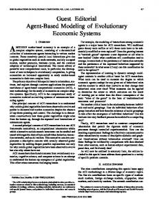
Fig. 2. Conceptual view of multidomain solutions: σ1 (HiTA), σ2 (MIDP), σ3 highest availability.

Suppose the average link availability is given by λ and the node availability is given by ν. Usually, a backup path is longer backuppathlength than a primary path. Call the ratio primarypathlength = φ ≥ 1. Let N be the number of traversed domains, and n the average number of hops for the primary path in each domain. We will not include the source and destination domain in these calculations, because they are (obviously) not included in SLAs. Fig. 2 shows three conceptual solutions. The first solution σ1 corresponds to a HiTA solution. Note that the two LSPs do not necessarily run through the same domains (not shown in picture). The second solution σ2 is a MIDP solution, which is logically reduced to a segment protected path. Solution σ3

Fig. 3.

2

3

4

5

Availability in function of N , n = 6

In Fig. 3 we show the relation between the availability of the connection and the number of domains. The number of nodes per domain is 6, λ = 0.999, ν = 0.99999, φ = 1.1 We immediately notice that MIDP solutions σ2 achieves higher availability than HiTA solutions σ1 , while both effectively provide protection for a single failure. For a single domain σ1 outperforms σ2 because it protects against the gateway failure. If ν = 1 both solutions have the same availability for a single domain. In Fig. 4 we show the relation between the availability of the connection and the number of nodes per domain. The number of domains is 3, again λ = 0.999, ν = 0.99999, φ = 1.1. If

1.0002

1 0.999987751 0.9998

σ1 0.9996

0.999626638

σ2 σ3

0.9994

0.9992 0.999020052 0.999 1

2

Fig. 4.

3

4

5

6

7

8

9

10

Availability in function of n, N = 3

we compare Fig. 3 for N = 5 and Fig. 4 for n = 10, we see that the primary path length for the end-to-end connection (N.n) is the same. σ1 has the same availability for both scenarios. The availability for the other solutions will drop slightly, because the number of segments will be less (and the segments therefore a bit longer). In short, we see that σ2 improves an order of magnitude (an extra 9) over σ1 and σ3 improves an order of magnitude over σ2 . The σ3 solution achieves ’five nines’ over 5 domains. IV. A PPLICABILITY To facilitate the goal of multidomain protection, we can impose some light requirements on each domain. One observation is that if you want a survivable connection over multiple domains, it’s only reasonable to require that each domain in itself can setup survivable connections between two internal nodes. This means that there must be the topological constraint of a 2-connected graph, allowing for at least 2 disjoint paths between any node-pair in the network. Another requirement on the network is that it must be possible to route your paths in a flexible way (as opposed to the shortest path routing common to the OSPF mechanism in classic IP networks). So, some basic traffic engineering is needed in each network. We will therefore continue with the formal requirement that each domain is a GMPLS-capable optical network with a 2connected physical topology.

Fig. 5.

Survivable Structure

An abstraction of the three optical paths in a single domain is shown in Figure 5. We have omitted the domain superscript δ.

A. Proof We will now prove that this structure is always possible in any 2-connected network, if all the gateway nodes (ip , is , e1 , e2 ) are chosen in the network and only the primary ingress (ip ) and secondary ingress (is ) are fixed. In other words, we can choose which of the egress gateways (e1 ,e2 ) will be primary (ep ) and the other egress will then be secondary (es ). Definition 4.1: A graph G is a pair G = (V, E) consisting of a set V 6= ∅ and a set E of two-element subsets of V . The elements of V are called vertices. An element e = ab ∈ E is called an edge with end vertices a ∈ V and b ∈ V . If V is finite, we call G a finite graph. Note that this definition specifies a simple (no parallel edges) undirected graph. A graph S = (V1 , E1 ) is called a subgraph of G = (V, E) ⇔ V1 ⊆ V ∧ E1 ⊆ E. A path is a non-empty graph P = (V2 , E2 ) of the form V2 = {v0 , v1 , . . . , vk } , E2 = {v0 v1 , v1 v2 , . . . , vk−1 vk }. In this paper, we will specify paths with a vertex list: P (v0 v1 . . . vk ). A cycle is a closed path, i.e. the end nodes v0 and vk are the same. We define the intersection of two paths, P1 ∩ P2 as the set of vertices Vi that are in both paths. If P1 ∩ P2 = ∅ we call P1 and P2 disjoint. If for two paths having the same end nodes P1 (a . . . b) ∩ P2 (a . . . b) = (a, b) then we also call these paths disjoint. If for any pair of vertices (v1 , v2 ) ∈ V 2 there exist k mutually node-disjoint paths between them, we call the graph k-connected and the connectivity κ(G) = k. In a k-connected graph, it will require the removal of at least k nodes to disconnect the graph into different components. A set of k nodes which disconnects the graph is called a set of cut–vertices. The k-connectedness of a graph does not imply it is always possible to construct disjoint paths between 2 given nodes successively. If it is not possible to find a disjoint path between two nodes after construction of a first path Pβ between them, we call Pβ a blocking path. It is easy to see that a blocking path must contain a set of cut–vertices. Theorem 4.1: Let G(V, E) be a graph on the set of vertices V with |V | ≥ 4 and connectivity κ(G) ≥ 2. If we choose four different nodes (ip , is , e1 , e2 ) ∈ V 4 , it is always possible to find three paths P , P B and B in G, that suffice one of the following two conditions: P (ip . . . e1 ) ∩ P B (ip . . . e1 ) = {ip , e1 } ∧ B (is . . . e2 ) ∩ {ip , e1 } = ∅

(9)

P (ip . . . e2 ) ∩ P B (ip . . . e2 ) = {ip , e2 } ∧ B (is . . . e1 } ∩ {ip , e2 } = ∅

(10)

Theorem 4.1 states the requirements for common pool interdomain connection in a formal way. The two conditions (9) and (10) are identical but the roles of e1 and e2 are reversed. Saying that one of the two conditions must be true is to state that ep and es can be chosen and ip and is are fixed.1 1 Note that due to symmetry, Theorem 4.1 also proves that e and e can be p s fixed and ip and is interchangeable. This could be useful for using backward propagation in signaling and setting up interdomain connections. In this paper, we focus on forward propagation.

Fig. 6.

Survivable Structure on a cycle (Lemma 4.2)

The conditions state that it is possible (a) to find two disjoint paths between ip and ep and (b) a path from is to es that does not cross ip or ep . The first condition is trivial, but in a 2–connected network it’s not trivially possible to specify two nodes which must be excluded from a path and find a solution. They can form a pair of cut–vertices. This is why both conditions (9,10) are included in the theorem, which will become clear in Lemma 4.2. Lemma 4.2: Theorem 4.1 holds if there is a cycle containing ip , e1 , is , e2 . Proof: If all nodes ip , e1 , is , e2 are on a cycle, it is immediately clear that the path P will follow one side of this cycle and that the path P B must span the other side of the cycle. Now, it is also easy to see that there are three distinct permutations of the gateway nodes which we must consider, since all others are rotations or mirror images of these. 1) ip − e1 − is − e2 . (Figure 6.a) In this configuration, we can choose the path P (ip . . . e1 ) not to contain any other gateways and the path P B (ip . . . e2 . . . is . . . e1 ) must then contain is and e2 . The path B (is . . . e2 ) can be chosen as the is − e2 subpath fully contained in P B. In this way, condition (9) is met. 2) ip − is − e2 − e1 . (Figure 6.b) We can setup the same paths as in the first option: we can choose the path P (ip . . . e1 ) not to contain any other gateways and again the path P B (ip . . . is . . . e2 . . . e1 ) (along the other side of the cycle) will contain is and e2 . The path B (is . . . e2 ) is the is − e2 subpath fully contained in P B, meeting condition (9). 3) ip − is − e1 − e2 . (Figure 6.c) It is impossible to satisfy condition (9): should

we consider the paths P (ip . . . is . . . e1 ) and P B (ip . . . e2 . . . e1 ), then B (is . . . e2 ) will either contain ip or e1 , which is a violation of the subcondition B (is . . . e2 ) ∩ {ip , e1 } = ∅. However, it is immediately clear that this configuration is the same as the second one, where e1 and e2 switched places. Following the same argument as above, we can therefore conclude that, the paths P (ip . . . e2 ) (not containing the other gateways), the path P B (ip . . . is . . . e1 . . . e2 ) and the P B–subpath B (is . . . e1 ) will satisfy condition (10).  With the result from Lemma 4.2, it is easy to prove Theorem 4.1. Given the four nodes ip , is , e1 , e2 in G, we can find 2 disjoint paths P and P B between ip and e1 , because of the 2–connectedness of G. This fulfills the first clause of condition (9) in Theorem 4.1. Similarly, we can find 2 disjoint paths Pq and Pr from is to e2 . The second clause of the requirement (9) states that there must be a path B from is to e2 not containing ip or e1 . This condition is met when one of the paths Pq and Pr does not contain ip or e1 and we choose B (is . . . e2 ) equal to this path. The only situation when B = Pq or B = Pr does not satisfy condition (9) is when both Pq and Pr run through either ip or e1 , but then all four nodes ip , is , e1 and e2 are on a cycle formed by Pq and Pr and, following Lemma 4.2, there are paths P (ip . . . e2 ), P B (ip . . . e2 ) and B {is . . . e1 ) that satisfy condition (10).  V. H EURISTIC SOLUTION Our proof of Theorem 4.1 immedialty gives rise to one algorithm for finding a suitable solution: first, we remove the nodes ip and ep = e1 from the graph G and compute B as the shortest path from is to es = e2 . If no such path can be found, remove ip and ep = e2 from the graph G and compute B as the shortest path from is to es = e1 , which then must exist. Then compute a pair of disjoint paths from ip to ep using the Suurballe algorithm to form P and P B. VI. S IMULATION RESULTS We will now compare our simple heuristic to an ILP solution computed using CPLEX 10 [14]. We have computed results for two networks. A first is the NSFNET backbone topology, which has 14 nodes and 21 links, the second is a pan-European network with 67 nodes and 120 links. A simulation selects 4 nodes (ip , is , ep , es ) at random and compares the ILP results to the heuristic. The top half of Table VI shows the results for 5 runs of 100 simulations for NSFNet. The table gives the relative performance of the ILP versus the heuristic (H). The middle column shows where the ILP and the Heuristic reach the same link usage, and the number in brackets shows matches, where the ILP and the heuristic have exactly the same solutions. We immediately notice that in 80% of the cases the solutions are equivalent. Also, sometimes the solver seems to perform worse than our heuristic. A reason why there could be so little variance in the solutions could be the restricted

!h ILP > H 10 15 12 18 14 15 17 20 18 22

RUN 1 2 3 4 5 1 2 3 4 5

ILP = H 84(2) 80(1) 82(0) 82(2) 80(1) 76(0) 71(0) 71(0) 72(0) 71(0)

Simplex solver) for NSFNet and the large network were 203ms and 26ms, for the heuristic it was below 1ms.

H > ILP 6 5 6 0 6 9 12 9 10 7

VII. C ONCLUSIONS

TABLE I S IMULATION ON NSFN ET AND A PAN -E UROPEAN N ETWORK

topology of the NSFNET network. To test this, we also ran a large simulation on the pan-European network described in [10]. Results are given in the bottom half Table VI. There is a bit more variation in the results, but the bulk of solutions have the same total link usage. We have not found exact matches in the ILP and heuristic for this network.

In this paper we have presented some properties of the common pool multidomain Resilience. We have noted that it lies in the MIDR class of multidomain solutions, and shown through analytical analysis that this class has the highest availability. We have given a proof that the solution can be computed in any 2-connected network, which is important for signaling such connections in real networks. This proof leads to an easily computable heuristic solution. We compared the heuristic to the ILP using simulations on two different networks. The results show that the heuristic produces results very close to the optimum. The ILP achieves slightly better results by increasing some paths in length to allow for more sharing. VIII. ACKNOWLEDGMENTS This work was funded by the European Commission through the NoE BONE and the Flemish fund for scientific Research, project FWO 3G057808. R EFERENCES

1600 1400 1200 1000 B

800

PB

600

P

400 200 0 ILP

H

Fig. 7.

ILP

H

ILP

H

ILP

H

ILP

H

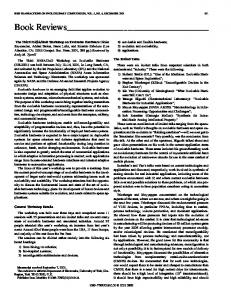
ILP vs. Heuristic, European Network

The relative gain of the ILP over the heuristic (H) is shown in Figure 7. Every bar shows the total link usage for 100 simulations, for each of the 5 runs. The length of the primary paths (P), the primary backups (PB) and the Backup (B) is shown in each bar. Every time the ILP has a small gain, and this is clearly accomplished by routing over longer primary paths (P) instead of using a shortest cycle, so the B has more opportunities to share resources with P and PB. We think the reason why the heuristic can outperform CPLEX, is the discrete value of the optimization goal and the large number of solutions with almost optimal values. We tried different solvers for CPLEX and with each the same solution value was achieved. When the ILP performed worse than H for the NSFNet, the difference was 1.04 on average. When the ILP outperformed H it was 1.15 better on average. On average, the ILP performs slightly better than the heuristic. Average computation time on an average PC (AMD Athlon 64, 3000+, 1GB RAM) for the ILP model (Using CPLEX 10, Network

[1] B. Puype, J.-P. Vasseur, A. Groebbens, S. De Maesschalk, D. Colle, I. Lievens, M. Pickavet and P. Demeester, Benefits of GMPLS for multilayer recovery, IEEE Commun. Mag., vol 43, no. 7, July 2005, pp. 51-59. [2] J. Hawkinson and T. Bates, Guidelines for creation, selection and registration of an Autonomous System, RFC1930, March 1996. [3] J.P. Vasseur, M. Pickavet and P. Demeester, Network Recovery, Protection and Restoration of Optical, SONET-SDH, IP and MPLS, Morgan Kaufmann Series in Networking, Elsevier, 2004. [4] J.W. Suurballe and R.E. Tarjan, A Quick Method for Finding Shortest pair of Disjoint Paths, Networks, vol. 14, 1984, pp. 325-36. [5] D. Stamatelakis, W.D. Grover, Theoretical Underpinnings for the Efficiency of Restorable Networks Using Pre-configured Cycles (p-cycles), IEEE Transactions on Communications, vol.48, no.8, August 2000, pp. 1262-65. [6] D.L. Truong and B. Jaumard, Recent Progress in Dynamic Routing for Shared Protection in Multidomain Networks, IEEE Commun. Mag., vol. 46, no. 6, June 2008, pp. 112-19. [7] A. Farkas, J. Szigeti and T. Cinkler, p-Cycle Based Protection Schemes for Multi-Domain Networks, Proc. DRCN 2005, 5th Int’l Workshop on Design of Reliable Communication Networks, Lacco Ameno, Island of Ischia, Italy. [8] D. Staessens, L. Depr´e, D. Colle, I. Lievens, M. Pickavet and P. Demeester, A quantitative comparison of some resilience mechanisms in a multidomain IP-over-Optical network environment, Proc. of ICC2006, the IEEE Int’l Conference on Communications, Istanbul, Turkey, 11-15 June 2006 [9] M. Pickavet, P. Demeester, D. Colle, D. Staessens, B. Puype, L. Depr, I. Lievens, Recovery in multilayer optical networks, Journal of Lightwave Technology, Vol. 24, no. 1, January 2006, pp. 122-34 [10] D. Staessens, D. Colle, I. Lievens, M. Pickavet, P. Demeester, W. Colitti, A. Nowe, K. Steenhaut, R. Romeral, Enabling high availability over multiple optical networks,IEEE Commun. Mag., vol. 46, no. 6, June 2008, pp. 120-26. [11] P. Cholda, A. Jajszczyk, Reliability Assessment of Optical p-Cycles, IEEE/ACM Transactions on Networking, Vol. 15, no. 6, Dec. 2007, pp.1579-92. [12] A. A. Akyamac¸, S. Sengupta, J.-F. Labourdette, S. Chaudhuri, S. French, Reliability in Single Domain vs. Multi Domain Optical Mesh Networks, Proc. NFOEC, Dallas TX, Sept. 2002. [13] E. E. Lewis, Introduction to Reliability Engineering, John Wiley & Sons, 1987. [14] ILOG CPLEX 10 www.ilog.com