Transients computation for relay testing in real-time - IEEE Xplore ...

IEEE Transactions on Power Delivery, Vol. 9, No. 3, July 1994

1298

TRANSIENTS COMPUTATION FOR RELAY TESTING IN REAL-TIME

J. K. Bladow, Member, D. M. Hamai

M. Kezunovit, Senior Member, M. Aganagit V. SkendiiC, Member, J. Domaszewicz, Student Member Texas A&M University U. s. A.

Abstract- This paper discussescharacteristicsof a new digital simulator for protection relay testing. The most demanding design requirement is computation of fault transients under the condition of real-time change of power system configuration due to relay operation. This problem is solved using EMTP computational techniques enhanced with novel numerical solutions for dynamic power system configuration change and nonlinear element modeling. An advanced computer architecture is utilized to achieve further optimization of the execution time for the transients computation code. The main advantage of this design is the use of conventional single processor computer architecture in combination with advanced digital signal processors (DSPs). This makes this simulator an off-the-shelf product with all the benefits of commercially available computers priced at a relatively low cost. Keywords: Digital Simulators, Relay Testing, Transients Computation, EMTP, Digital Signal Processing INTRODUCTION The use of digital simulators for relay testing has been known since the early eighties [l].A number of different designs have been introduced over the last ten years [2-6]. These simulators have been proven to be very accurate and flexible tools for relay testing [7].However, one limitation of the mentioned designs was difficulty in performing relay testing in real-time. Digital simulators of an open-loop type are extremely effective in producing fault transients and replaying either simulated or recorded transients into relays for testing purposes. Nevertheless, if the relay testing requires multiple dynamic changes of the power system configuration based upon the relay’s response, the open-loop simulators can not easily be utilized to support transient computations under these real-time constraints. A need for a new simulator design exists for the cases where EMTP computations and configuration changes are performed under a closed-loop control of a relay under test. Several recent papers have investigated fast methods for transients computation [8-lo]. It has been argued that parallel computer architectures are needed to meet the real-time computation requirements [9,10]. These feasibility study results are encouraging for future implementations of real-time digital simulators for relay testing. A complete design of a simulator for relay testing using a parallel architecture has been demonstrated using custom designed solution [ll]. That im-

S. M. McKenna Western Area Power Administration

plementation is very important since it proved the validity of a parallel architecture approach. This paper describes the development of a new digital simulator with very stringent implementation requirements. The use of commercially available computer architectures was imposed against the use of a customized design solution. This was considered the main design requirement and was imposed to be able to take advantage of full system software and hardware support and upgrades readily available for commercial computer products. Yet another demanding requirement was the need to model rather involved power system configuration consisting of nonlinear elements such as MOVs and surge arresters as well as instrument transformers such as CTs and CCVTs. It has also been required that the transients computation is performed at a 50-100 ps time step for most of the test cases.

A new simulator design has been implemented to meet these rather demanding requirements. This paper reports on the implementation results for transients computation. This was the most challenging part of the design since it asked for quite innovative implementation approaches. The first part of the paper is devoted to a brief overview of the design requirements. The system architecture selected for the simulator implementation is discussed next. Real-time techniques utilized for transients computation related to the network reconfiguring and simulating the nonlinear components are then presented. Performance evaluation results for the implementation of real-time transients computation are given at the end.

IMPLEMENTATION REQUIREMENTS The simulator implementation was aimed at developing a commercial grade digital system capable of computing fault

transients for relay testing in real-time. This general goal has been expanded into several specific requirement categories discussed below.

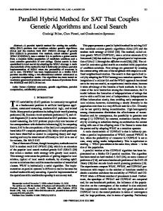
Computation of Network Transients This requirement category has been defined based on a typical Western Area Power Administration 345 kV network section as shown in Figure 1.

93 SM 383-0 PWRD A paper recommended and approved by the IEEE Power System Relaying Committee of the IEEE Power Engineering Society for presentation at the IEEE/PES 1993 Summer Meeting, Vancouver, B.C., Canada, July 18-22, 1993. Manuscript submitted January 12, 1993; made available for printing April 5, 1993.

Fig. 1. WAPA Reference System

PRINTED IN USA

0885-8977/94/$04.00 0 1993 IEEE

1299

A close analysis of this network produced very demanding transients computation constraints that are summarized in Table I.

I ,

-1

h

Table I. Network Modeling Requirements Nonlinear Components

MOVs, CCVTs, CTs, Arresters

Simulation Events for Relay Testing

faults, autoreclosing seauences. symphatetic trips on parallel ’ lines,fault reversals, propaga-

I

- -

V

Fig. 2. Digital Simulator Architecture

It is important to note that this selection of the c o m p nents has satisfied the main design requirements including the most important one of using commercially available hardware.

Simulator Interfaces Two major groups of requirements are related to the user interface and the relay interface. It waa specified that the user shall be provided with means for building network models through a graphical user interface. This meant that a on-line diagram interface be provided. Also, the user shall be capable of calculating component and network parameters automatically. This required standard implementation of line constants and transformer auxiliary routines as well as development of custom routinesfor steady-state calculations and automatic network equivalencing. The graphical user interface solution represents a powerful tool for relay testing and had to be implemented, as in some other simulator applications, using custom designed techniques based upon commercially available packages [3,11]. A detailed description of the Graphical User Interface will be reported in a separate paper to be published in the near future. Protection relay test interface requirements are very similar to the ones specified during development of an open-loop version of the simulator [6,7]. The main difference in the realtime version is the larger number of relay terminals to be tested and the improved data acquisition solution to be used for realtime sensing of contact changes. The simulator described here is designed for simultaneous testing of up to three relay terminals. The real-time constraint for interaction between the simulator and the relay is a particularly difficult requirement to meet since it gsks not only for a fast computation of transients, but also for correspondingly fast 1/0 data transfer support. This paper concentrates primarily on the solution of the fast computation of transients while the real-time 1 / 0 data transfer support is not presented in detail and will be discussed in a separate paper.

SYSTEM ARCHITECTURE After an extensive feasibility study, it was decided that the simulator architecture given in Figure 2 would be implemented. As it can be seen from Figure 2, the simulator system is made of the following major components: 0

IBM RISC 6000, Model 320 supportingthe Graphical User Interface

0

IBM RISC 6000, Model 580 supporting the real-time computation of network transients

0

2 Digital Signal Processing (DSP) boards, containing two TMS320 C40 processors each, supporting the real-time computation of instrument transformer transients Waveform reconstruction subsystem supporting real-time 1/0 interaction between the simulator and the relays under test

0

The waveform reconstruction subsystem hardware has been developed as a part of a different project [6] and was tailored for the real-time digital simulator applications. It has unique performance characteristics as specified in Tables I1 and 111. This subsystem is now being produced by a major amplifier vendor and is expected to be commercially available in the near future. Table 11. Waveform Reconstruction Subsystem Main Specifications

1. Number of Reproduced Bits 2. Sample Rate 3. Output Impedance

1! I1 -

4. Analog Bandwidth 5. Output Signal Range

I

I

I I 6. No. of Analog Channels 7. No. of Digital Channels 8. Channel

* **

16 Fs=3.2 to 25 kHz Voltage Channels: < 152 Current Channels: 50052; DC to 1 kHz I > >50052; DC 4 0.45 fs Volt age Channels: > f32OV#eor; f0.2Apeo1. Current Channels: -

-

#.,.,.A

I . a m 1 7

I12 Voltage

+ 12 Current*

J Vpeok

3 sets of 4 voltage and 4 current channels each. 3 sets of 16 input and 16 output channels each.

Table 111. Waveform Reconstruction Subsystem Additional Specifications

I# I

8’

ITEM

Interface

I

SPECIFICATION

3#/208 V; 60 Hz RS 422 Serial Link with TMS320 C30 Data Format

1

I11 Y

I

1300

~',CI

RTS to GUI Communication

Network

Transformers

DSP 2 - R T Instrument

The RTS implementation departed from the EMTP by shifting, as much as feasible of the computation burden to a preparatory phase. This was made possible using the fact that the real-time requirement applies only to the computations that are to be performed at each of the successive time steps. Thus, for example, at each time step the nodal equation:

Instrument

RT RTS

-RealTime - Real Time System

Fig. 3. Real-Time Subsystem Organization The organization of the simulator subsystem devoted to real-time transients computation is given in Figure 3. As it can be observed, the three digital signal processors (DSPs) are used to interface to the three relay terminals, while the fourth DSP is used as a real-time manager for 1/0interfacing between the RISC 6000, Model 580 and the remaining DSPs. The RISC machine is used for computation of network transients while the three DSPs are used for computation of instrument transformer transients. The following sections give details of the transients computation implementation and the performance evaluation.

COMPUTATION OF NETWORK TRANSIENTS This section gives implementation details of some of the most demanding requirementsthat relate to network codguration changes and nonlinear component modeling. Performance evaluation results are also discussed.

General Approach to Network Modeling

A new C program called RTS (the real-time system) has been developedfor the network transients computation. One of the main principles of RTS development was to use the EMTP modeling and solution techniques [12]. The following system components are modeled in the RTS: e Uncoupled branches: R, L, C and R - L e Coupled R - L branches e &circuits for short lines representation e Constant parameter overhead transmission lines e Tkansmission lines with frequency dependent parameters e Voltage sources e Faults 0 Relays 0 Switches 0 Series capacitors with MOV protection 0 Surge arresters e Instrument Transformers: CTs and CCVTs

is solved where [GIis the matrix of node conductances, and [v(t)] and [h(t)]-vectors of nodal voltages and current sources at the time t , respectively. In the RTS, the equation (1) is solved as:

where A denotes the nodes with the unknown voltages and B the nodes to which voltage sources ( e B ) are connected. The inverse of [GAA]is kept in an explicit form, and the forcing function F B ( ~is) precomputed by the preprocessor outside the time loop. The advantage of precomputing of the forcing function should be rather clear having in mind that the submatrix is typically very sparse, as its only nonzero elements correspond to the internal impedances of the sources. The advantage of keeping the inverse in the explicit form will be more evident in what follows. The nature of the simulator operation is such that it requires frequent changes in the network topology. The EMTP approach, which calls for a retriangularization of the nodal conductance matrix, is not viable as it cannot be performed fast enough. Modeling of nonlinear components for the RTS necessitates further approximationsover the ones used in the EMTP. In particular, a new approach had to be developed to deal with series capacitors with MOV protection in a less demanding way than the Newton-Rapson technique used in the EMTP. The following sections give details of the implementation for these most difficult simulator computational requirements.

Switches and Network Configurations Switches are modeled as time-controlled switches of the EMTP with the exception that they present a small positive resistance (typically 1.e - 3 to 1.e - 4n) when closed and the infinite resistance when opened. The main reason for this departure is to be able to keep the number of the network nodes constant during the run enabling one to easily carry the history current injections across all the possible network configurations that may arise. Now, suppose that a switch closes, connecting nodes i and j . Then, the new matrix can be expressed as:

[a

The branches and transmissionlines are modeled the same

N Y as in the EMTP. Voltage sources and the forcing functions are represented in the form of look-up tables whichhave to be long enough to hold at least one full cycle of the corresponding functions. Faults are introduced by closing a switch at a prespecified incidence angle. If a fault is of a temporary nature, then the user needs to specify the time at which the switch will open. Relays are associated with the switches they act upon. This association also determines which voltages and currents are to be outputted. Modeling of the switches and the nonlinear elements is described in the following sections.

(3) where

1 -1 0

if if if

k=i k=j,k=l, k#i,j

...,I AI

(4)

1301 and where g is the (large) switch admittance. G is nonsingular then 80 is [GI:

(

if the rank 1-update matrix I+g[G]-'

[eij] [eij]

9-l

exists.

By a well known result of Sherman-Morrison-Woodburry 3 the rank 1-update matrix exists if, and only if, 6 = 1 +g [eij] [GI-' [eij] # 0 (in ow case, 6 2 1, as [GI is a symmetric positive semi-definite matrix and g > 0), and

Finally, one gets the formula for updating switch:

[aafter closing a

Observe that the rank 1-vector on the righthand side of (7) is just the difference of the two columns of [GI-'

If the matrix is block diagonal, that the matrix update is confined to a block to which the end nodes of the switch belong. The blocks appear as a result of decoupling introduced by transmission lines. The rows and columns of the matrix [G'l are conformally permuted by a preprocessor so as to produce a block diagonal matrix. Only the elements of the diagonal blocks are stored. This provides for a very significant saving in execution time. Furthermore, it should be noted that there are no numerical problems with the above formula even if g becomes very large. The right hand side can be correctly computed even for an infinite g, but in that case, it becomes singular. The reason for requiring that it be finite has a different background. Namely, if g were allowed to be infinite then the above operation would become irreversible. Otherwise, the same formula (with -g in place of g) is applied to reopen the switch. Again, if the resulting matrix is well conditioned, there are no numerical difficulties.

TV

Fig. 5. Idealized MOV Characteristics

The varistor is assumed to behave in accordance with the idealized characteristicsshown in Figure 5. Thus, as long as the voltage U across the capacitor is below a preset value V, the component is viewed as just a capacitor. If the voltage exceeds the V level, the above characteristics are inserted in parallel to the capacitor and stays there aa long as the condition persists. This is described by the following equation:

In addition, the bypass switch protects the MOV by closing if the energy dissipated in the MOV becomes greater than a user defined level. Figure 6 shows the characteristics of an actual MOV (five segment exponential characteristics)superimposed on its approximation which was used in the test runs. The ideal MOV characteristicsused should be a good a p proximation of the actual one around the point at which the MOV is expected to operated. This is the main guideline for choosing the parameters V and r (V = 190KV and r = 1R in this case).

The change in [ q - ' resulting from an MOV operation is carried out implicitely using the equation (7). Namely, instead of updating the matrix, only a correction of the nodal voltages is computed.

Series Capacitors with MOV Protection The difficulty of protecting a series compensated line with MOV protection is well known [13]. It is also known that an MOV represents a demanding computational burden [14]. A series capacitor with an MOV and a switch is treated just as a single component. This component is shown in Figure 4.

Z n O m n r m 1.41

C Fig. 4. Series Capacitor with MOV Protection

Fig. 6. Comparison of an Actual MOV Characteristics with the Approximation used in ElTS

1302 COMPUTATION OF INSTRUMENT TRANSFORMER TRANSIENTS As mentioned earlier, one of the important requirements for the transients computation is that the simulator produes not only correct network transients but also appropriate instrument transformer transients. In order to deal with a complex nonlinear modeling problem for the current transformer (CT) and the capacitor coupling transformer (CCVT), an approximative approach has been undertaken. The simplified CT and CCVT models utilized are still quite accurate as has been demonstrated earlier [15,16]. The implementation of the CT and CCVT models has been performed on dedicated DSP boards as shown in Figure 3. The computations are performed in parallel to the ones carried out for the network transients. This provides for the full utilization of the simulator architecture by performing network transients computation on the RISC 6000 machine and computation of the instrument transformer transients (4 CCVTs and 4 CTs per testing terminal) on a dedicated DSP engine.

Current Transformer (CT) Modeling '

The CT topology is simplifed [17]as shown in Figure 7.

Rs, Ls-Burden Fig. 7. Simplified CT Circuit Topology The circuit contains nonlinear flux versus current relation. Due to the nonlinearity, a complete solution of the circuit equations would require an iterative procedure every time step, which would be unacceptable for real-time computation. To avoid a one time step delay in handling, a piecewise linear approximation of the flux versus current curve, shown in Figure 8, has been adopted.

4 Am.

astart

Capacitor Coupling Voltage Transformer (CCVT) Modeling

A typical topology for CCVT modeling 1151 is presented in Figure 9.

Fig. 9. CCVT Circuit Topology The major issue in CCVT modeling is the degree of simplification one wants to pursue. While many approaches are possible, two extreme cases are implemented for evaluation purposes. The first case is baaed on the fact that the discretized circuit given in Figure 9 is a gth order linear system. As such, it can be represented with a gth order infinite impulse response (IIR) filter, or by a difference equation with, at most, 17 product terms. This is the ideal form for implementation on the DSP since one product term can be handled in a single instruction cycle. It should be noted that in the IIR approach, state variables are linear combinations of currents and voltages that exist in the circuit, and as such, do not have direct physical meaning. Only the output voltage is available as a physical quantity. Also, this approach is useless if any nonlinearity is introduced into the circuit.

In order to make a more conservative assessment of the computation time, the other case in which the circuit given in Figure 9 is directly solved, is also implemented. In this case, all currents and voltages in the circuit are directly available as program variables.

PERFORMANCE EVALUATION This section gives results from various test cases implemented for transients computation evaluation. The cases selected are quite critical for relay testing and, therefore, r e p resent a good example of the simulator performance. The performance evaluation is carried out with two goals in mind. One is to observe the computation time needed to obtain transients and the other one is to observe the accuracy of the transients generated by the computations. The computation time achieved is compared with the one specified as the design requirement. The shape of the transients obtained is.compared to the one generated by the EMTP. Therefore, the computation time requirements and the EMTP simulations were used as the criteria for performance evaluation.

Fig. 8. Piecewise Linear Approximation of Flux versus Current Curve

Computation of Network Transients

The resulting computations are now reduced to the following steps:

Simulator performance, when computing network transients, has been evaluated using the following three cases derived from the WAPA system given in Figure l:

0

Solving equations describing the linear part of the system

0

Searching the piecewise linear characteristic to find out which segment the current (or the flux) is in. The slope of the segment will be used in the first step during the next it erat ion.

0

0

Case 1: A network with 42 nodes used to evaluate the simulator's capability to handle complex network configurations in real-time. Case 2: A network with 6 MOVs used to evaluate simulator's capability to handle a large number of MOV operations in real-time.

1303 Case 3: A network with dynamic switch operations used to evaluate simulator's capability to handle change of network configurations in real-time. The network configurations for the three cases are given in Figure 10. Description of the test cases and the transients computation timing are given in Table IV for all the cases. In all the computations, a 50ps time step was used. Comparison of the waveforms generated by RTS and EMTP is @en in Figure 11 where applicable.

A number of test runs have been performed using the IBM RISC 6000, Model 550 machine which is presently available for the development. The test results demonstrate the simulator's capability to compute transients with a time step close to 100 ps in all the cases. However, once the Model 580 machine becomes available, most of the tests cases shown would execute with a time step around 50 p s . Since the final simulator implementation is based on the use of the Model 580, it can easily be seen that the simulator capability satisfies the requirement that the simulator shall be able to compute transients for the WAPA system in real-time with time steps in t b range of 50-100 ps.

Glen Canyon

s2,

\-

Fig. lO(c). WAPA Network Configuration for Test Case 3. a

XlW

.

.

.

.

.

.

.

.

.

Table IV. Test Cases and Timing Results ~

1 o m 0.01 0.01s om oms o.m 0.035 0.01 0.015 Fig. ll(a). Comparison of EMTP and RTS simulation Results; The voltages at Node (*)-Phase B (Case 1) '0

* This includes a total of 33 MOV operationsover lo00 time steps.

** Sequence of Events: (1) hult: SLG-Phase B at 0.05 (2) S1 to open at 0.1 s; (3) S2 to open at 0.11665 s.

s;

Fig. ll(b). Comparison of EMTP and RTS Simulation Results; Voltage Across the Phase A Series Capacitor of the Upper Line in Fig. 10(b) (Case 2)

Glen Canyon

Fig. 10(a). WAPA network Configuration for test Case 1.

1

4 Flagstaff

Glen Canyon I

I

11

Fig. 10(b). WAPA Network Configuration for Test Case 2.

-251

o

'

0.02

'

0.01

"

0.06

0.08

ai'

'

0~12 0.14

.

0.16

I 0.18

Fig. Il(c). Case 3: Voltage at the Fault Location

0.2

1304 Computation of Instrument Transformer Transients

I

As mentioned earlier, up to 4 CT and 4 CCVT models are assigned to a single DSP engine, reducing the number of required processors to three. This section analyzes the following two implementation approaches: 0

Using TMS320 C30 DSP

0

Using TMS320 C40 DSP

The TMS320 C30 DSP implementation has been carried out in the fist stage of the simulator design while the C40 DSP has been selected for the final implementation. The main difference is in the input clock frequency which is 33 MHz for the C30 and 50 MHz for the C40. This means that the instruction cycle time T is 60 ns and 40 ns, respectively. The program for instrument transformer transients computation is implemented in the assembly language. It is carefully coded to take advantage of the processor architecture. The following performance evaluation shows computation time and errors of the transients for both CT and CCVT. CT computation time is found to be 16T for the equation solution and 24T for the segment search. The cumulative time for both steps is 40T. For the CCVT, the IIR approach requires 17T for the 17 product terms and 8T for setting up data structures. The total time required is 25T. The direct solution approach for CCVT transients computation requires 117T. A summary of the results obtained for both C30 and C40 implementations is given in Table V. These results indicate that an iteration of 4 CTs and 4 CCVTs can easily be computed in a small fraction of the time step of 50-loops. Table V. Execution Time for an Iteration of Instrument Transformer Transients Computation (in p s )

A

f r i 111

Fig. 13. CCVT Correctness Verification Results;(a) Secondary Voltage as Computed by TMS320 C30, (b) Difference Between Reference and Assembly Language Implementations Magnified lo3 Times 12 and 13. The wave shapes of the transients almost overlap for the two different implementations. The differences are extremely small, as can be observed from the scale of the difference signal. CONCLUSIONS The results presented in this paper demonstrate how the design of the new simulator has met some of the most critical implementation requirements. The following are some most important aspects of the real-time transients computation capability of the simulator: The performance of the IBM RISC System 6000,Model 580 and TMS320 C40 processors demonstrates that a realtime simulator for relay testing can be built using commercial computer products.

A new approach to simulationof the network switching enA comparison of the wave shapes generated by the programs implemented on DSP and using the EMTP approach with a comesponding integration rule is presented in Figures

ables the required real-time interaction between the relay and the simulator. Proposed modeling of the nonlinear network components such as MOVs, CTs and CCVTs, uses new approximations. The precision obtained with this approach is suitable for the simulator application and yet the real-time computation is achieved. ACKNOWLEDGEMENTS The study reported in this paper has been funded by DOE-Western Area Administration under contract FC65-90WA 07990. The authors want to acknowledge the participation of Drs. H. W. Dommel and J. Marti from the University of British Columbia and Dr. A. Abur from Texas A&M University in the Phase I of this project where the feasibility study of the simulator implementation was carried out.

0.01

0.02

am

0.w

OM

0.06

T h [I]

Fig. 12. CT Correctness Verification Results; (a) Secondary Current as Computed by TMS320 C30, (b) Difference Between Reference and Assembly Language Implementations Magnified lo‘ Times

REFERENCES [l] A. Williams, R. H. J. Warren, “Method of Using Data From Computer Simulationto Test Protection Equipment,” IEE Proceedings, Vol. 131, Pt. C, No. 7, November 1984. [2] J. Esztergalyos, et. al., “Digital Model Power system,” IEEE Computer Applicatiotu in Power, Vol. 3, No. 3, July 1990.

1305 [3] P. Bornard, et. al., “Morgat: A Data Processing Program for Testing Transmission Line Protective Relays,” IEEE I)urnsactions on Power Delivery, Vol. 3, No. 4, October 1988. [4] M. A. Redfern, et. al., “A Personal Computer Based System for the Laboratory Evaluation of High Performance Power System Protection Relays,” IEEE Transactions on Power Delivery, Vol. 6, No. 4, October 1991. [5] M. Koulischer, et. al., “A Comprehensive Hardware and Software Environment for Development of Digital Protection Relays,” Intl. Conf. on Power system Protection ’89, Singapore, 1989. [6] M. Kezunovit, et. al., “DYNA-TEST Simulator for Relay Testing, Part I: Design Characteristics,” IEEE !bansactions on Power Delivery, Vol. 6, No. 4, October 1991. [7] M. Kezunovit, et. al., “DYNA-TEST Simulator for Relay Testing, Part I1 Performance Evaluation,” IEEE I)urnsactions on Power Delivery, Vol. 7, No. 4, July 1992. [8] D. M. F’alcm, et. al., “Application of Parallel Processing Techniquesto the Simulation of Power System Electromagnetic Transients,” IEEE PES Winter Meeting, Paper No. 92WM 287-3-PWRS, New York, January 1992. [9] R. C. Durie, C. Pottle, “An Extensible Real-Time Digital Transient Network Analyzer,” IEEE PES Winter Meeting, Paper No. 92WM 175UPWRS, New York, January 1992. [lo] K. Werlen, H. Glawitsch, “Computation of “kansients by Parallel Processing,” IEEE PES Summer Meeting, Paper 92SM 465-5-PWRD, Seattle, July 1992. [ll]P. G. McLaren, et. al., ”A Real-Time Digital Simulatorfor Testing Relays,” IEEE Bansactions on Power Delivery, Vol. 7, No. 1, January 1992. [12] Electromagnetic Transient Program (EMTP) Rule Book, EPRI EL 6421-1, Vol. 1, 2, June 1989. [13] R. J. Martila, “Performance of Distance Relay Mho Ekments on MOV-Protected Series-Compensated Transmission Lines,” IEEE Transactions on Power Delivery, Vol. 7, No. 3, July 1992. [14] J. R. Lucas, P. G. McLaren, “A Computationally Efficient MOV Model for Series Compensation Studies,” IEEE Bansactions on Power Delivery, Vol. 6, No. 4, October 1991. [15]M. Kezunovit, et. al., “Digital Models of Coupling Capacitor Voltage Transformers for Protective Relay Transient Studies,” IEEE Bansactions on Power Delivery, Vol. 7, No. 4, October 1992. [16] M. Kezunovit, et. al., “ExperimentalEvaluation of EMTP Based Current Transformer Models for Protective Relay Transient Study,” IEEE PES Winter Meeting, Paper No. 93WM 0414PWRD, Columbus, February 1993. [17] W. L. A. Neves, H. W. Dommel, “On Modeling Iron Core Nonlineaxities,” IEEE PES Winter Meeting, Paper No. 92WM 176-&PWRD, New York, 1992.

M. KezunoviC (S’77, M’80, SM’85) received his Dipl. Ing. degree from the University of Sarajevo, Yugoslavia, the M.S. and Ph.D. degrees from the University of Kansas, all in electrical engineering in 1974, 1977, and 1980, respectively. Dr. Kezunovit’s industrial experience is with Westinghouse Electric Corporation in the U. S. A., and the Energoinvest Company in Yugoslavia. He also worked at the University of Sarajevo, Yugoslavia. He was a Visiting Associate Professor at Washington State Uqiversity in 1986-1987. He has been with Texas A&M University since 1987 where he is an Associate Professor.

M. AganagiC received his Dipl. Ing. degree in electrical engineering from the University of Sarajevo and M.S. degree in computer science from the University of Nis, Yugoslavia in 1970 and 1973, respectively. In 1975 he received his Ph.D. degree in operations research from Stanford University. Until joining Texas A&M University as a research scientist in 1992, Dr. Aganagit was with the Energoinvest Company, Sarajevo, where he held different positions in the Research and Development Division. His main research interest lies in the area of mathematical programming and its applications to power systems. V. Skend2iC (M’88, S’90) received his Dipl. Ing. degree from the University of Split, and M.S. degree from the University of Zagreb, Yugoslavia, all in electrical engineering, in 1983 and 1990, respectively. From 1984 to 1989 he was with the Electrical Engineering Department at the University of Split. currently he is a graduate student at Texas A&M University.

J. Domaszewicz (S’89) received his M.Sc.E.E. degree from Warsaw Technical University, Poland, in 1986. &om 1986 to 1989 he was with the Department of Electronics at Warsaw Technical University. Mr. Domaszewicz is currently a graduate student at Texas A&M University. J. K. Bladow was born in Moorhead, Minnesota in 1959. He earned both Bachelor and Master degrees (power option) in electrical engineering from North Dakota State University. Mr. Bladow joined the Western Area Power Administration (Western) in January 1983, and has held various technical and managerial positions. Mr. Bladow currently is Western’s Assistant Administrator for Washington Liaison. Mr. Bladow has been involved with Electromagnetic Transient Program (EMTP) studies, the application and setting of protective relays, system short-ircuit studies, substation electrical design, and major electrical equipment specifications. Mr. Bladow is a member of the IEEE and a registered professional engineering in Colorado. S. M. McKenna was born in Spokane, Washington in 1951. He earned his B. S. degree from the Colorado School of Mines in 1978. Mr. McKennajoined the Western Area Power Administration (Western) in September 1980. Mr. McKenna is currently in the Substation Control Branch where he is involved in control system design for advanced technology devices, protective relaying application and testing, and power system testing. Mr. McKenna is a registered professionalengineer in Colorado.

D. M. Hamai was born in San Rafael, California on October 14, 1963. He received his B.S. degree in electrical engineering from the University of Colorado in 1986. Mr. Hamai has been employed with the Western Area Power Administration since 1986 and is currently in the Technical Branch where he is involved with various Electromagnetic Transients Program (EMTP) studies, power system protection applications, and major power equipment requirements.

1306 DISCUSSION J. R. MARTI, L. LINARES, H. W. DOMMEL (University of British Columbia, Vancouver, B. C., Canada): The authors are to be commended for advancing the real-time simulator of Phase I of the WAPA project and suggesting interesting techniques for the representation of MOVs and switching operations. We would like to use this opportunity to ask the authors for clarification of some aspects regarding the models and results presented in the paper. 1) Even though Woodbury’s technique to update the [GI-’ matrix after switching operations is more efficient than a full retriangularization ( -N2 operations versus -N3 ), it still adds extra processing time to the calculations in the time step. Similarly, the modelling of MOVs as illustrated in Fig. 5 of the paper requires additional overhead time when the MOVs start conducting. Table IV in the paper indicates average calculation times per solution step and not the larger calculation times needed during switching or MOV operations. In CASE 2, for example, the larger solution times needed during the 33 MOV operations are masked out when taking the average over 1000 time steps. This observation also applies to the switching operations in CASE 3. For the practical application of the simulator in relay testing, it is very important, in order to avoid jitter in the signals applied to the relays, that the output samples be at equal time intervals. This means that the actual useful bandwidth of the simulator is determined by the largest solution times and not the average times indicated in Table IV In this regard, even though it might be conceivable to skip one solution step during circuit breaker operation (switching), the validity of this approach would be more questionable in the case of MOV operations. Could the authors comment on this issue and indicate what the largest solution times were for the cases of Table IV? 2) It is stated in the paper (third paragraph after Eq. (8)) that MOV operations do not require a modification of the [GI-’ matrix of the network. The MOV model used by the authors, however, has a finite resistance r when the MOV branch begins to conduct. Topologically, this means that a new branch is added to the network when the MOV starts to conduct (if it was assumed totally open before conduction) or that the parameters of a branch in the network change value (if the MOV was represented by a high resistance before conduction). This means that regardless of the approach used to define the network equations, the topological parameters of the network change when the MOV branch starts to conduct. This, in turn, implies a change in the corresponding coefficients of the equations defining the relationships between voltages and currents in the network, and not just a change in the independent constraintsvector (“righthand side”) as seems to be implied in the paper. Could the authors clarify this issue and explain more specifically the kind of corrections introduced in the solution equations to simulate the MOV operations? 3) In our experience with the real-time simulator, and in the experience of other researchers, to attain the timings indicated in Table IV for CASE 1 requires the unrolling of indexed loops by hand-coding explicit assignment instructions to avoid subscript calculations and memory access overheads. Unfortunately, this hand-crafting limits the generality of the solution since the code has to be rewritten as the power system components change. Could the authors indicate whether this is the case for the RTS code used to run CASE 1 in Table IV, and also if any non-ANSI-C features or Assembly routines were used in the code? In closing these comments, we would like to reiterate our congratulations to the authors of this paper for their interest in advancing techniques towards achieving a workstation-based real-time network simulator. Manuscript received August 10,1993.

,

M. KezunoviC, M. Aganagid, V. SkendiiC Texas A&M University, College Station, Texas; S. McKenna, DOE-Western Area Power Administration, Golden, Colorado: We would like to thank the discusser on a set of interesting questions giving us the opportunity to further describe the main features of our design.

1. We agree with the reviewers that the possibility of skip ping one or more solution steps in order to accommodate fluctuations in the simulation time step is unacceptable for relay testing applications. Furthermore, we feel that any violation of the stringent sampling clock jitter requirements (& Ins in the TAMU simulator) must be reliably detected, and followed by an immediate simulation shutdown. The hardware and software mechanisms designed to efficiently satisfy this requirement deserve separate attention, and their description is currently being prepared for publication. In the meantime, some of the simulator architecture implementationaspects can be found in 111. A number of profding runs was performed in order to verify the simulator real time operation. Typical timing results measured on an actual communication link interface connecting the RS6000/580 with the TMS320C40 DSPs are shown in Figure 1. Each point on the graph represents the time needed to calculate a single solution step, and send the results over to the DSP subsystem. As pointed out by the discussers, the computation time increases for both MOV operations, and switch updates. By analyzing the results given in Figure 1, it can be seen that every switch operation incurs a single step time increase in the order of 18ps. The MOV operation is somewhat cheaper ( X 3ps per device), but extends over the entire period of MOV activity. Using these times in a naive real-time design would result with the fastest simulation time ing limited to x 87ps. This bottleneck can be avoided by recognizing time delays associated with circuit breaker components used in an actual power systems. Depending on the breaker type, the delays can range from 1 to several cycles, giving an ample time margin for additional computational load balancing. In the TAMU system, the breaker models are allocated to one of the DSP processors, enabling this device to buffer simulation results before passing them to the waveform reconstruction system. This mechanism effectively decouples the simulation time from the output subsystem time step. Actual simulation 90 Longest Timc Step = 86.5

*N-

Fig. 1. Results of

Typical Simulation Step Calculation Times

~

1307

is effectively being run “ahead” of real time for a time period allowed by a given breaker model. In a typical case, assuming a 2 cycle breaker, results will effectively be averaged over the breaker mechanical response time interval % 19.6ms (>300 time steps) [2]. In the case o f data in Figure 1, this effectively means that the real-time simula~ ~ step. tion can successfully be executed with a 6 4 . 7 time The outlined procedure makes it possible to use. an average execution time measurements for precise performance prediction of the TAMU simulator.

2. We have not been implying that the computation of an MOV can be accomplished without a modification of the matrix [GI-’. On the contrary, we begin the third parare graph after eq. (8) by stating “The change in [q-’ sulting from an MOV operation is carried out implicitly using the equation (7).” Here is how. h m (7), it follows that voltages can be computed as: H-’[h]=

This shows that the effect of an MOV operation (and hence, solution of the modified network equations) can be achieved at the expense of just additional multiplications, where is the rank of the corresponding block submatrix. So we do take into account the change of the topology, but we do it without explicitly changing the underlying matrix. Two further remarks are in order here: 0

0

The voltage correction is performed on individual diagonal blocks so n is typically much less than N, where N is the rank of matrix G . The implicit modification technique pays off in all the cases when an MOV conducts for less than 2n successive time steps.

3. The RTS code does not contain a single line of an msem bly code. It was entirely coded in the standard ANSI-C language, and relies only on the standard AIX Services (IBM UNIX implementation). Advanced code optimization techniques have been used extensively throughout. There was no “hand-crafting” that would compromise the program generality.

References Note that the last factor on the right hand side is e q d to:

([G]-’[eij])T[h] = [eij]T[G]-’[h] = [eijlT[w]= vi - W , Hence:

*

(vi - v j )

- [GI;’) ‘4 = ‘1 - 1 + g [ e i j l ~ [ q - l [ e i ,([GI? l

111 M. Kezunovic et. al., “A New Multiprocessor Architecture Implementation of a Real-Time Simulator for Power

System Applications,” ISCA International Conference on Computer Applications in Industry and Engineering, Honolulu, Hawaii, December 1993.

[2] R 0. Berglund, et. al., “One Cycle Fault Interruption at 500 kV-System Benefits and Breaker Design,” IEEE T-PAS, September/October 1974,p. 1240-1251. Manuscript received October 11, 1993.