flow consists of finding velocity and wave pressures un- der assumption ... Navier-Stokes equations for incompressible inviscid fluid. ..... An album of fluid motion.
of a local wave number in time and space compared to the wave elevation. This assumption allows the use of special derivative formula ζz = kζ, where k is the wave number; using this formula the solution is constructed. In twodimensional case the solution is given by
Computation of pressures in inverse problem in hydrodynamics of potential flow
1 ∂φ e−I(x) |x,t = − √ ∂x 1 + α2
0
∂ z/∂z ˙ + αα˙ I(x) √ e dx, 1 + α2 (2)
Zx
Ivan Gankevich
Zx
I(x) =
Alexander Degtyarev
∂α/∂z dx, 1 + α2
0
Abstract
where α is the wave slope. In three-dimensional case the solution is given by
The inverse problem in hydrodynamics of potential flow consists of finding velocity and wave pressures under assumption that a wavy surface elevation is known beforehand. The solution to this problem in both two and three dimensions is known but is based on theory of smallamplitude waves. Since some hydrodynamic problems involve waves of arbitrary amplitudes a more general solution is needed. In the paper such solution is given for two and three dimensions and it is shown that it is efficient from computational point of view and more accurate than the solution for small-amplitude waves.
� ∂2φ � ∂2φ ∂2φ 1 + αx2 + 2 1 + αy2 + 2αx αy + 2 ∂x ∂y ∂x∂y � � ∂αx ∂αx ∂αx ∂φ + αx + αy + ∂z ∂x ∂y ∂x � � ∂αy ∂αy ∂αy ∂φ + αx + αy + ∂z ∂x ∂y ∂y ∂ ζ˙ + αx α˙x + αy α˙y = 0. ∂z Here the formula is not explicit and represents elliptic equation which is intended to be solved by a variety of known numerical methods. Although, these methods are efficient and work well for a wide range of wavy surfaces some weather conditions produce waves with wave numbers which change frequently in time and space. These are transitions between normal and storm weather, wind wave and swell heading from multiple directions and some others. These weather conditions and a possibility to obtain a more general solution are the main reasons for solving the potential flow problem for arbitrary amplitude waves case.
INTRODUCTION A potential flow is the flow of inviscid incompressible fluid which is described by the system of equations [2] ∇2 φ = 0, p 1 φt + |~υ |2 + gζ = − , 2 ρ Dζ = ∇φ · ~n,
at z = ζ(x, y, t),
(1)
at z = ζ(x, y, t),
where φ is velocity potential, ζ is wavy surface elevation, p is wave pressure, ρ is water density, ~υ = (φx , φy , φz ) is velocity vector, g is gravitational acceleration and D is a substantial derivative. The first two equations are equation of continuity and equation of motion (the so called dynamic boundary condition) and both are derived from Navier-Stokes equations for incompressible inviscid fluid. The last one is kinematic boundary condition for free wavy surface which states that rate of change of wavy surface elevation equals to the change of velocity potential derivative along the wavy surface normal. In previous paper [1] the solution to inverse problem is given for small-amplitude waves when wave length is much larger than wave height (λ � h). It is shown that the inverse problem is linear and can be reduced to a Laplace equation with a mixed boundary condition with equation of motion being used only to determine wave pressure. The assumption of small amplitudes means the slow decay of wind wave coherence function, i.e. a small change
1
TWO-DIMENSIONAL CASE
For two-dimensional flow equation (1) can be rewritten as follows. φxx + φzz = 0, � 1 2 p φt + φ + φ2z + gζ = − , 2 x ρ ζx ζt + ζx φx = p φx + φz , 1 + ζx2
at z = ζ(x, t), at z = ζ(x, t).
The first step is to solve Laplace equation using Fourier method. The solution can be written as integral similar to Fourier transform: Z∞ φ(x, z) = −∞
1
E(λ)eλ(z+ix) dλ.
(3)
Then coefficients E can be determined by plugging this integral into kinematic boundary condition and evaluating derivatives. This step gives equation ζt p = 1 − iζx + iζx / 1 + ζx2
Z∞
ing form: Z∞ Z F (x, y) =
E(λ) =
1 1 2πi λ
−∞
Z∞ −∞ Z∞ −∞
−∞
(λ, γ) → (r, θ), λ = r cos θ, γ = r sin θ, |J| = r,
ζt p e−λ(ζ+ix) dx. 1 − iζx + iζx / 1 + ζx2
the formula is rewritten in polar coordinates for both f and F: Z∞ Z2π F (ρ, ψ) = 0
1 λ(z+ix) e dλ λ
(7)
(x, y) → (ρ, ψ), x = ρ cos ψ, y = ρ sin ψ,
rf (r, θ)eirρ cos(ψ−θ)+rζ(ρ,ψ) dθdr.
0
Then applying additional transformations
(5)
0
0
r → r0 , r = er ; ρ → ρ0 , ρ = e−ρ ; 0
ζ → ζ 0 , ζ = e−ρ ζ 0
ζt p e−λ(ζ+ix) dx. 1 − iζx + iζx / 1 + ζx2
(8)
to the radius vectors and function ζ a convolution can be obtained:
When equation (1) is solved that way wave pressures can be determined from dynamic boundary condition. Since velocity potential is the only unknown prerequisite for determining wave pressures it is feasible to use it to validate the solution. A comparison was done to the known small-amplitude wave solution (2) and numerical experiments showed good correspondence rate between resulting velocity potential fields. In order to obtain velocity potential fields the wavy sea surface was generated by autoregressive model differing only in wave amplitude. In numerical implementation infinite outer and inner integral limits of (5) were replaced by the corresponding wavy surface size (x0 , x1 ) and wave number interval (λ0 , λ1 ) so that inner integral of (5) converges. Experiments were conducted for waves of both small and large amplitudes and in case of small-amplitude waves both solutions produced similar results, whereas in case of large-amplitude waves only general solution produced stable velocity field (Figure 1). The fact that velocity fields for small-amplitude waves are not equal can be explained by stochastic nature of autoregressive wind wave model (i.e. the amplitude is small in a statistical sense only). Therefore, general solution in twodimensional case works for different wavy sea surfaces without restriction on a wave amplitude.
2
dλdγ.
(6) In order to derive inversion formula this expression should be reduced to a two-dimensional convolution. By applying transformations
λE(λ)eλ(ζ+ix) dλ,
(4) The third step is to plug (4) into (3) which yields the final result: 1 φ(x, t) = 2πi
λ2 +γ 2
−∞
which represents forward bilateral Laplace transform and thus can be inverted to yield formula for coefficients E: Z∞
√ f (λ, γ)ei(λx+γy)+ζ(x,y)
F (ρ0 , ψ) = f1 ∗ f2 , 0
f1 (r , θ) = e
2r 0
(9)
0
f (r , θ), h i 0 0 f2 (ρ0 , ψ) = exp ie−ρ cos ψ + e−ρ ζ 0 (ρ0 , ψ) .
Since convolution theorem permits any converging integral transform to be applied to a convolution, here a modified polar version of Fourier transform 0
Z∞ Z2π
F {g(r, θ)}(r1 , θ1 ) = 0
−e−2r g(r, θ)
0
� � exp −ie−r r1 cos(θ1 − θ) dθdr
(10)
is used. Applying this transform to the both sides of equation (9) yields the final formula � � f (x, y) F {exp [ix + ζ(x, y)]} , F{F (x, y)} = F x2 + y 2 (11) where F is ordinary forward Fourier transform. This formula is useful in two cases. First, it allows inversion of initial modified Fourier transform (6) which is needed when solving three-dimensional problem. Second, it can be used to compute F efficiently with use of fast Fourier transform family of algorithms. So, special transform is the tool to solve three-dimensional problem.
SPECIAL TRANSFORM
3
Three-dimensional problem can be solved with help of special inversion formula which serves as a modified version of Fourier transform. The transform has the follow-
THREE-DIMENSIONAL CASE
Three-dimensional problem is solved mostly the same way as its two-dimensional counterpart, however, special transform developed in the previous section should 2
u(x)
u(x)
u1(x) u2(x)
2 0 -2
u1(x) u2(x)
2 0 -2
0
30
60
90
0
30
60
x
90
x
Figure 1: Comparison of velocity fields produced by general solution (u1 ) and solution for small-amplitude waves (u2 ). Velocity fields for small-amplitude (left) and large-amplitude (right) wavy sea surfaces. and (8) from previous section are applied:
be used instead of bilateral Laplace transform and some terms from system of equations (1) should be rewritten in dimensionless form for convolution to be physically feasible.
Z∞ Z2π ζt = 0
3.1
dθdr0 eM e
r 0 −ρ0
(iN cos(θ−ψ)+ζ) M e
2r 0
N d0
0 0
E(r0 , θ)[N 3 −ieρ cos(θ − ψ)ζρ0 (d0 − N )
Formula derivation
0
−ieρ sin(θ − ψ)ζψ (d0 − N )],
Consider a square region with a side N where the problem is being solved. Then coordinate transform (x, y) → (xN, yN ) produces system of equations with dimensionless x and y:
r � � where d = N 2 + e2ρ0 ζρ20 + ζψ2 . 0
Finally, after applying modified Fourier transform (10) to the both sides of this equation the formula for coefficients E can be derived: � � n o E(λ, γ) M (iN x+ζ) F {ζt (x, y)} = F F f (x, y)e , λ2 + γ 2 � �q N 2 + ζx2 + ζy2 − N N 2 + iζx q f (x, y) = M . N N 2 + ζx2 + ζy2
1 1 φxx + 2 φyy + φzz = 0, N2 N ! φ2y 1 φ2x p 2 φt + + 2 + φz + gζ = − , 2 N2 N ρ at z = ζ(x, y, t), ζt +
ζx ζy ζx ζy φ x + 2 φy = φx + φy + φz , 2 N N Nd Nd at z = ζ(x, y, t),
3.2
q where d = N 2 + ζx2 + ζy2 . The first step is to solve Laplace equation with Fourier method which yields Z∞ Z φ(x, y, z) =
√ E(λ, γ)eM (iN (λx+γy)+z
λ2 +γ 2 )
Using formula (11) the integral from (12) can be decomposed into two forward and one inverse Fourier transforms, so the whole solution can be computed efficiently: � n � � o� E(λ, γ) M (iN x+ζ) −1 F e . φ(x, y, z) = F F λ2 + γ 2
dλdγ.
−∞
(12) Here λ and γ represent wave numbers which were made dimensionless with transform (λ, γ) → (λM, γM ). Then the expression is plugged into the kinematic boundary condition yielding Z∞ Z ζt =
√ dλdγE(λ, γ)eM (iN (λx+γy)+ζ
Numerical implementation
Forward and inverse Fourier transform of E cancel each other: ( ) � F {ζt (x, y)} F eM (iN x+ζ) −1 � φ(x, y, z) = F . F f (x, y)eM (iN x+ζ)
λ2 +γ 2 )
There is no easy way to derive analogous formula for velocity potential derivatives, however, numerical experiments have shown that there is no need to do it. These derivatives can be obtained numerically via finite difference formulae. Less number of integral transforms means less numerical error and faster computation.
−∞
i M h 3p 2 N λ + γ 2 − iλζx (d − N ) − iγζy (d − N ) . Nd In order to obtain convolution formula transformations (7) 3
0.5
0.5
υ
υ
0.36 0.0
0.0
0.72
-0.72 0.72
0.54
-0.54
0.36
-0.36
z
z
-0.72 -0.5
-1.0
-0.5
0.54
-0.54
-1.0
-0.36 -1.5
0
1
2
3
4
5
-1.5
6
0
1
2
x
3
4
5
6
x
Figure 2: Slices at y = 3.1, t = 0 of propagating waves’ velocity potential field (left) and stream lines (right). Here ζ(x, y, t) = 41 cos(4πx − 0.25t).
1.0
1.0
0.5
0.5
0.0
0.3
z
z
-0.4 0.4 -0.31
-0.31
-0.5 0.4
-0.5
0.4 0.2
-0.2
-0.2
-1.0 0.2 -1.5 0
-0.5
-0.4
0.0
-1.0
0.2 1
2
3
4
5
-1.5
6
x
0
1
2
3
4
5
6
x
Figure 3: Slices at y = 3.1, t = 1 of standing waves’ velocity potential field (left) and stream lines (right). Here ζ(x, y, t) = cos(4πx) sin(−0.25t).
Figure 4: Slice at y = 3.1, t = 0 of propagating Figure 5: Slice of a wavy surface with waves of large amwaves’ velocity potential stream lines. Here ζ(x, y, t) = plitude generated by autoregressive wind wave model. 1 2 cos(4π(x + y) − 0.25t).
4
So, from computational point of view velocity potential is given by four fast Fourier transforms plus three numerical differentiations (one for each coordinate), in other words its asymptotic complexity is roughly 4n log2 n + 3n, where n is the total number of points in the volume.
3.3
For large amplitude waves the solution was tested on the wavy surface generated by autoregressive wind wave model and in this case the shape of stream lines and potential field is asymmetric. As can be seen in Figure 5 stream lines are skewed in the direction which is opposite to the direction of wave propagation.
Evaluation
CONCLUSIONS
Three-dimensional solution was evaluated on different types of waves: propagating, standing and real ocean waves generated by autoregressive model. For the first two types of waves the shape of velocity potential and velocity field is known and can be found elsewhere [4], so they were used to validate the solution. The last type of wave was used to see how the solution behaves in case of large amplitude waves. Since computation is done with discrete Fourier transforms the resulting data is sometimes perturbed on the edges [3]. In real world those perturbations should be removed from the solution but here they were left for the sake of transparency of results. Propagating waves are known to have region of negative velocity potential under the front slope and region of positive potential under the back slope while standing waves are known to have region of negative potential under their crests and region of positive potential under their bottoms. Velocity of a water particle is always in the direction of negative potential and it is perpendicular to the contours of velocity potential. This behaviour is fully captured by the solution (Figures 2–4).
To sum up, new solution allows determining velocity field for waves of arbitrary amplitudes and is fast from computational point of view. For plain waves the solution gives the same field as previously known solutions and for largeamplitude waves it gives asymmetrical velocity field.
REFERENCES [1] A. Degtyarev and I. Gankevich. Evaluation of hydrodynamic pressures for autoregression model of irregular waves. In Proceedings of 11th International Conference on Stability of Ships and Ocean Vehicles, Athens, pages 841–852, 2012. [2] N. Kochin, I. Kibel, and N. Roze. Theoretical hydrodynamics [in Russian]. FizMatLit, 1966. [3] Richard G Lyons. Understanding digital signal processing. Pearson Education, 2010. [4] Milton Van Dyke. An album of fluid motion. 1982.
5