This paper presents a method to compute Mean and Gaussian curvatures from range images. The rst and second partial derivatives are estimated by.
Computation of Surface Curvature from Range Images Using Geometrically Intrinsic Weights 1) T. Kurita 1)
and
Electrotechnical Laboratory
1-1-4 Umezono, Tsukuba, Japan 305
Abstract This paper presents a method to compute Mean and Gaussian curvatures from range images. The rst and second partial derivatives are estimated by the weighted least squares t of a biquadratic polynomial within a local moving window. The weights are determined on the basis of surface distances and normal angular distances from the center points of the window. 1.
Introduction
In recent years, range image (depth map) processing has become one of the most important topics in computer vision research. The main reason is that the quality of the digitized range data has been improved by the developments of active and passive range sensing techniques (for example, [8]). Range data provide explicit geometrical information about the shape of visible surfaces. Using this basic information, some problems in 3-D object description and recognition are easier to solve. Especially, one can obtain dense range maps very e�ectively using active range nders. Besl and Jain [1] have proposed an attractive idea for surface characterization from the point of view of di�erential geometry. Mean and Gaussian curvatures (surface curvatures) are invariant under rigid transformation. Smooth surfaces are locally characterized by them and are classi ed into one of eight surface types using a combination of their signs. Thus, if we could compute local surface curvatures accurately, one would be able to segment range images into several surface regions with similar surface types called the topographic primal sketch [6]. Since di�erential geometry is a theory for smooth di�erentiable surfaces, one must take into account the fact that real range images have discontinuities (depth and orientation) which will in uence the computation of the curvatures. In order to prevent this problem Fan [5] proposed to detect discon-
P. Boulanger
2)
2)
National Research Council Canada Ottawa, Canada K1A 0R6
tinuities rst and then do a local curvature measurement. Yokoya [9] proposed a method which employs a selective surface t. The best local window which provides a minimum tting error among the covering windows is selected and is used for curvature estimation. Boulanger [3] proposed a new smoothing lter for range images which is invariant to viewpoint and is capable of preserving depth and orientation discontinuities. The lter employs two new surface distance, one is the length of the minimum trajectory joining two points on the surface, and the second one is the normal angular distance, which is de ned as the average angular variation of the normal vector along the minimum trajectory joining two points on the surface. In this paper, the rst and second partial derivatives are determined by the weighted least squares t of a biquadratic polynomial within a local moving window based on these distances. The present weighting method assigns small weights for the points which are not geometrically compatible with the center point of the window. Thus, the derivatives are estimated mostly based on the points which are compatible with the center point. Since the distances across a discontinuity are large, small weights are assigned to points which are on the other side of that discontinuity. Then, surface curvatures are computed from these derivatives according to the de nitions. In section 2, we review the concept of intrinsic surface distance and normal angular distance. Then an algorithm to compute these distances within a window is presented. In section 3, we show how to use these distances to do a weighted least squares t. In section 4, we show experimental results of Mean and Gaussian curvature computation using our method and then compare it with the results produced by a non-weighted least squares method.
2.
Surface and Normal Angular Distance
In this section, we will brie y review concepts of di�erential geometry [4], and then de ne the notion of intrinsic surface distance and normal angular distance[3]. We will also present an algorithm to compute these distances within a window.
2.1. Di�erential Geometry of Range Images Usually, range data is presented in the form of a real matrix z (x; y ). Consider a graph surface, namely the graph of a di�erentiable function z = h(x; y), where (x; y) belong to an open set U � R2 . Let us parametrize the surface by
�(x; y) = (x; y; h(x; y)); (x; y) 2 U:
(1)
Then the rst and second partial derivatives are
�x = (1; 0; hx ); �y = (0; 1; hy ); �xx = (0; 0; hxx ); �xy = (0; 0; hxy ); �yy = (0; 0; hyy ): Thus the surface normal at the point (x; y ) is given
by
� ^� (0hx ; 0hy ; 1) N (x; y) = x y = j�x ^ �y j (1 + h2x + h2y )1=2 ;
(2)
where ^ denotes the vector product. The Gaussian and mean curvatures are
hxx hyy 0 h2xy ; (3) (1 + h2x + h2y )2 (1 + h2x )hyy + (1 + h2y )hxx 0 2hx hy hxy (4) : H = 2(1 + h2x + h2y )3=2
K =
2.2. Surface and Normal Angular Distances Consider a curve �(t) on a surface. The arc length s� between two points p = �(tp ) and q = �(tq ) along the curve is given by
s� (p; q) =
Z
tq
tp
j�0 (t)jdt:
(5)
Since only the z -values are available on discrete points of the (x; y ) coordinate for a digitized range image, we must have a discrete form of equation (5) to compute the arc length between two points along the curve. Let us consider a partition of a curve �(t) de ned as �(ti ); tp = t0 < t1 < . . . < tk < tk+1 = tq . If the steps of the piecewise approximation are su�ciently
small, one can approximate the curve by a linear equation of the form
�(t) = (x(ti )+ai (t0ti ); y(ti )+bi (t0ti ); z(ti )+ci (t0ti )); (6)
)0x(ti ) where ai = x(tit+1 and bi and ci have similar i+1 0ti
expressions based on y and z . Then the derivative �0 (t) of � with respect to t is given by
�0 (t) = (ai ; bi ; ci ) for ti < t < ti+1 : Thus a discrete approximation of the arc length between p and q is given by
s� (p; q) =
k q X i=0
a2i + b2i + c2i :
(7)
This is equivalent to a polygonal approximation of the surface. Then the surface distance dS , namely the minimum distance among all trajectories joining the two points, is de ned by
dS (p; q) = min� s� (p; q):
(8)
Note that the value of dS will be large if the minimum trajectory goes across a depth discontinuity. However, this distance is not very sensitive to orientation discontinuity. Therefore, it is necessary to consider another distance which is sensitive to the change of surface orientation. The normal angular distance is de ned as the average angular variation of the normal vector along the trajectory joining the points p and q by
dA (p; q) =
1
Z
tq
(tq 0 tp ) tp
cos01 (< N (tp ); N (t) >)dt;
(9) where N (tp ) is the normal vector at tp . From the de nition (9), it is obvious that dA (p; q) is equal to zero if the normal vector along the trajectory is constant. If, however, the trajectory goes across an orientation discontinuity, the value of dA will be large. Moreover, this measure is also independent to viewpoint. The discrete form of equation (9) is given by
dA (p; q) =
k 1X
k i=1
cos01 (< N (t0 ); N (ti ) >): (10)
2.3. Algorithm to Find Minimum Trajectory To obtain surface distances from the center point to the other points in a moving window, we need to nd minimum trajectories from the center point to
all other points in the window. From the de nition (8), we can design an e�cient algorithm by using Single-Source Shortest Paths Algorithm for weighted graphs (for example, see [7]). The vertices of the graph correspond to the points in the window and the edges represent neighboring connections of points. From the equation (7), the arc length of the edge between points (x(ti ); y (ti )) and (x(ti+1 ); y (ti+1 )) is given by
q
a2i + b2i + c2i :
The running time of this algorithm is O((jE j + jV j)logjV j), where jE j denotes the number of edges.
In order to compute the normal angular distance, we need to estimate the surface normal at each point. In the following experiments, we used the estimates obtained by a least squares tting of a plane within local 3 by 3 windows (for example [3]). Once we have estimates of the surface normal, the normal angular distance is easily computed by tracing the minimum trajectory obtained by the previous algorithm. 3.
Mean and Gaussian Curvatures Computation
In this section, we will describe how to compute weights from these distances and how to apply this weight function to curvature computation.
3.1. Geometrical Weights To assign large weights for points which are geometrically compatible with the center point of the window and small weights for points which are not compatible, we use Gaussian weights based on the surface and normal angular distances. For surface distance dS (p; q), the weight wS (q ) is de ned by
d2 (p; q) wS (q) = exp(0 S 2 ); 2� S where p is the center point of the window and �S is a scaling parameter. For normal angular distance dA (p; q), the weight wA (q) is de ned by
d2 (p; q) wA (q) = exp(0 A 2 ); 2� A
where is a parameter to account for the relative importance of the normal angular distance with respect to the surface distance. The present weights have the following attractive properties:
�
The weights are independent of the viewpoint. In particular, they preserve local curvature information.
�
Larger weights are assigned for the points which are geometrically more compatible with the center point.
�
The weights are sensitive to both depth and orientation discontinuities. Thus, small weights are assigned to points which are in the opposite side of a discontinuity.
3.2. Surface Fitting Once we have the weights, the computation of derivatives is straightforward. It is common to t a second-degree surface to an L by L window centered at each point of the range surface, where L is usually odd. To t a surface, we use the weighted least squares method. The partial derivatives of the tting surface at the center of the window are taken as the estimates of the partial derivatives of the range data at that point. Let the range image depth values inside the window be denoted by hk ; k = 1; . . . ; N (N = L2 ) and let the weights of corresponding points be wk ; k = 1; . . . ; N . Let the tting second-degree surface be h^ (x; y) = a1 + a2 x + a3 y + a4 x2 + a5 xy + a6 y 2 : (12) The coe�cients of the tting surface are determined such that the weighted squares error
"2 (a) =
N X k=1
wk jhk 0 h^ k j2
(13)
is minimized. The optimum coe�cients vector a is given by a = (X T W X )01 X T W h;
(14)
where a = (ai ), h = (hk ), W = diag(wk ), and
2 3 1 x1 y1 x21 x1 y1 y12 5: ... X =4 2 1 xN yN x2N xN yN yN
3.3. Mean and Gaussian Curvatures
where �A is also a scaling parameter. By combining these two weights, we have
d2 (p; q) + d2A (p; q) w(q) = wS (q)wA (q) = exp(0 S ); 2� 2
(11)
The partial derivatives of the tting surface at the center of the window are given by
hx = a2 ; hy = a3 ; hxx = 2a4 ; hxy = a5 ; hyy = 2a6 :
Acknowledgments
The authors would like to thank M. Rioux, L. Cournoyer, and J. Domey of the National Research Council of Canada who kindly provided access to the range image database. References
Figure 1. Mean and Gaussian curvatures estimated by the present algorithm. (a) Mean curvatures. (b) Gaussian curvatures.
[1] P.J. Besl and R.C. Jain,\Invariant Surface Characteristics for 3D Object Recognition in Range Images", Comp. Vision, Graphics, and Image Processing 33, 33{80 (1986). [2] P. Boulanger and P. Cohen,\Stable Estimation of a Topographic Primal Sketch for Range Image Interpretation," Proc. of IAPR Workshop on CV{ Special Hardware and Industrial Applications Oct. 12{14, Tokyo (1988).
Figure 2. Mean and Gaussian curvatures estimated by the non-weighted least squares tting. (a) Mean curvatures. (b) Gaussian curvatures. These are considered as the estimates of the partial derivatives at the object's surface point. By using these derivatives, the surface normal at the point is computed from equation (2). The Gaussian and mean curvatures are also easily obtained from equations (3) and (4). 4.
Experimental Results
In this section, we present experimental results of Mean and Gaussian curvature computation and compare them with those obtained by the usual method based on non-weighted least squares. Figure1 (a) and (b) are the Mean and Gaussian curvature maps estimated by the present algorithm. In this computation, we used 5 by 5 windows and set the parameters as � = 1:5 and = 20:0. Figure2 (a) and (b) show the Mean and Gaussian curvature maps computed by the usual nonweighted least squares tting of a biquadratic polynomial. The size of the moving window was also 5 by 5. One can see the improvements of the curvature computation by using the geometrical weights, especially near discontinuities.
[3] P. Boulanger and P. Cohen,\Adaptive smoothing of range images based on intrinsic surface properties," Proc. of the SPIE Technical Symposium on Optical Engineering and Photonics in Aerospace Sensing,Orlando, FL April 16{20 (1990). [4] M.P. do Carmo,\Di�erential Geometry of Curves and Surfaces," Prentice-Hall (1976). [5] T.J. Fan. \Describing and recognizing 3-D objects using surface properties", PhD thesis, Institute for Robotics and Intelligent Systems, School of Engineering, University of Southern California, Los Angeles, California, August 1988. [6] R.M. Haralick, L.T. Watson, and T.J. La�ey. \The topographic primal sketch", Int. J. Robotics Res. 2(1): 50{72; 1983. [7] U. Manber, \Introduction to Algorithms, A Creative Approach," Addison-Wesley (1989). [8] M. Rioux, F. Blais, J.A. Beraldin and P. Boulanger, \Range image sensors development at NRC laboratories", Proc. of the Workshop on Interpretation of 3D scenes, Austin, TX, November 27{29 (1989). [9] N. Yokoya and M.D. Levine,\Range Image Segmentation Based on Di�erential Geometry: A Hybrid Approach," IEEE Trans. on Pattern Anal. Machine Intell., vol. PAMI{11, no. 6, pp. 643{649 (1989).