either direct numerical simulation (DNS) or large eddy simulation (LES); scatter- ..... the boundary conditions for a smaller DNS domain shown above. . . 99.
COMPUTATIONAL AEROACOUSTICS OF COMPLEX FLOWS AT LOW MACH NUMBER
A DISSERTATION SUBMITTED TO THE DEPARTMENT OF MECHANICAL ENGINEERING AND THE COMMITTEE ON GRADUATE STUDIES OF STANFORD UNIVERSITY IN PARTIAL FULFILLMENT OF THE REQUIREMENTS FOR THE DEGREE OF DOCTOR OF PHILOSOPHY
Yaser Khalighi June 2010
© 2010 by Yaser Khalighi. All Rights Reserved. Re-distributed by Stanford University under license with the author.
This work is licensed under a Creative Commons AttributionNoncommercial 3.0 United States License. http://creativecommons.org/licenses/by-nc/3.0/us/
This dissertation is online at: http://purl.stanford.edu/gj871wv3443
ii
I certify that I have read this dissertation and that, in my opinion, it is fully adequate in scope and quality as a dissertation for the degree of Doctor of Philosophy. Parviz Moin, Primary Adviser
I certify that I have read this dissertation and that, in my opinion, it is fully adequate in scope and quality as a dissertation for the degree of Doctor of Philosophy. Sanjiva Lele
I certify that I have read this dissertation and that, in my opinion, it is fully adequate in scope and quality as a dissertation for the degree of Doctor of Philosophy. Meng Wang
Approved for the Stanford University Committee on Graduate Studies. Patricia J. Gumport, Vice Provost Graduate Education
This signature page was generated electronically upon submission of this dissertation in electronic format. An original signed hard copy of the signature page is on file in University Archives.
iii
iv
Abstract Designing quiet mechanical systems requires an understanding of the physics of sound generation. Among various sources of noise, aerodynamic sound is the most difficult component to mitigate. In practical applications, aerodynamic sound is generated by complex flow phenomena such as turbulent wakes and boundary layers, separation, and interaction of turbulent flow with irregular solid bodies. In addition, sound waves experience multiple reflections from solid bodies before they propagate to an observer. Prediction of an acoustic field in such configurations requires a general aeroacoustic framework to operate in complex configurations. A general computational aeroacoustics method is developed to evaluate noise generated by low Mach number flow in complex configurations. This method is a hybrid approach which uses Lighthill’s acoustic analogy in conjunction with source-data from an incompressible calculation. Flow-generated sound sources are computed by using either direct numerical simulation (DNS) or large eddy simulation (LES); scattering of sound waves are computed using a boundary element method (BEM). In this approach, commonly-made assumptions about the geometry of scattering objects or frequency content of sound are not present, thus it can be applied to a wider range of aeroacoustic problems, where sound is generated by interaction of complex flows with solid surfaces. This new computational technique is applied to a variety of aeroacoustic problems ranging from sound generated by laminar and turbulent vortex shedding from cylinders to realistic configurations such as noise emitted from a rear-view side mirror and a hydrofoil. The purpose of each test case, in addition to validation of the method, is to explore various physical and technical aspects of the problem of sound generation v
by unsteady flows. Through these test cases, it is demonstrated that the predicted sound field by this technique is accurate in the frequency range in which the sound sources are resolved by the computational mesh. It is also shown that in computation of sound, acoustic analogies are less sensitive to numerical errors than direct computations. Finally, a discussion on the efficacy of LES and the effect of sub-grid scale dynamics on predicted sound is presented.
vi
Acknowledgments First and foremost, I would like to acknowledge my advisor, Professor Parviz Moin for his seamless support, patience and encouragement during the course of this work. I specifically appreciate his diligence in supporting fundamental research of the highest academic quality and industrial practicality. Dr. Meng Wang introduced me to the subject of computational aeroacoustics in the early stages of this work; his profound knowledge of turbulence and acoustics has been a crucial factor in forming the foundations of this research. I have been greatly inspired by his immense passion for science. I would also like to thank Dr. Daniel Bodony for many useful discussions and suggestions in the development of the boundary element technique. I have been privileged to have Dr. Ali Mani as my senior colleague, classmate, and friend during graduate school years. He has made critical contributions in this work on many levels. Many of ideas in this work were initiated from invaluable discussions with Ali. The development of the aeroacoustic module would not have been possible without the help of Dr. Frank Ham. The aeroacoustic module is developed within the CDP infrastructure which he has brilliantly developed. He has significantly influenced this work by his thorough knowledge of flow physics, numerical methods and computer science. I have benefited from many graduate courses on fluid mechanics, acoustics, and turbulence taught by Prof. Saniva Lele. Particular thanks go to him for his exemplary teaching style and his refreshing mathematical approach to fluid mechanics problems. I am indebted to my colleagues, office mates, and friends for their support on vii
a personal and technical level as well as for providing many great memories during my graduate studies. Warm thanks to Mohammad, Lee, Sanjeeb, Carlo, Seongwon, Charbel, Curtis, Matt, Jon, Simon, Donghyun, Jeremy, Mahnoosh, Hedi, Abtin, Shirin, Mazhar, Laleh, and Maryam among other friends. Thanks are also due the staff members of Building 500: Deb, Sara, Marlene, Annie, and Steve. Comments from Hilda Gould, Laurie Gibson, and Cutris Hamman on this manuscript are greatly appreciated. Financial support for this work was provided by the Office of Naval Research, the Franklin and Caroline Johnson Graduate Fellowship, and General Motors corporation. Finally, I would like to thank my beloved family. From my early years, my parents who are both physics instructors fostered in me a passion for fundamental science. They made many sacrifices to provide me with the opportunity to study overseas and achieve my dreams. My brother, Yashar, deserves a very special thanks for his lifetime mentorship, endless support, and love.
viii
Contents Abstract
v
Acknowledgments
vii
Nomenclature
xxi
1 Introduction
1
1.1 Motivation and objectives . . . . . . . . . . . . . . . . . . . . . . . .
1
1.2 An aerocoustics framework for complex flows . . . . . . . . . . . . . .
2
1.3 Studying various aeroacoustic problems . . . . . . . . . . . . . . . . .
7
1.4 Accomplishments . . . . . . . . . . . . . . . . . . . . . . . . . . . . .
9
2 Mathematical formulation
11
2.1 Derivation of acoustic analogy . . . . . . . . . . . . . . . . . . . . . .
12
2.2 Integral operators . . . . . . . . . . . . . . . . . . . . . . . . . . . . .
17
2.2.1
Inner product and corresponding identities . . . . . . . . . . .
17
2.2.2
Adjoint Helmholtz operator and reciprocity . . . . . . . . . .
18
2.2.3
Multipole integral operators . . . . . . . . . . . . . . . . . . .
19
2.3 Integral equation . . . . . . . . . . . . . . . . . . . . . . . . . . . . .
22
2.4 Hybrid approach for low Mach number flows . . . . . . . . . . . . . .
24
2.5 Structure of the aeroacoustics code . . . . . . . . . . . . . . . . . . .
28
2.6 Dimensional analysis . . . . . . . . . . . . . . . . . . . . . . . . . . .
31
2.7 Verification methods . . . . . . . . . . . . . . . . . . . . . . . . . . .
40
2.8 Utilizing hydrodynamic wall pressure . . . . . . . . . . . . . . . . . .
40
ix
2.9
Integration with an acoustic projection method . . . . . . . . . . . .
3 Numerics and singularity
43 47
3.1
Discretization of hybrid method . . . . . . . . . . . . . . . . . . . . .
47
3.2
Treatment of singular integrals . . . . . . . . . . . . . . . . . . . . . .
49
3.2.1
Evaluation of (D)0 . . . . . . . . . . . . . . . . . . . . . . . .
53
3.2.2
Evaluation of (Q)0 . . . . . . . . . . . . . . . . . . . . . . . .
54
Treatment of singular frequencies . . . . . . . . . . . . . . . . . . . .
55
3.3
4 Validation 4.1
4.2
4.3
57
Sound generated by laminar flow over a cylinder . . . . . . . . . . . .
57
4.1.1
Flow validation . . . . . . . . . . . . . . . . . . . . . . . . . .
59
4.1.2
Acoustic validation . . . . . . . . . . . . . . . . . . . . . . . .
60
4.1.3
Effect of background convection . . . . . . . . . . . . . . . . .
67
4.1.4
Effect of viscosity . . . . . . . . . . . . . . . . . . . . . . . . .
68
Sound generated by turbulent flow over a cylinder . . . . . . . . . . .
71
4.2.1
Flow validation . . . . . . . . . . . . . . . . . . . . . . . . . .
72
4.2.2
Acoustic validation . . . . . . . . . . . . . . . . . . . . . . . .
77
4.2.3
Budget analysis . . . . . . . . . . . . . . . . . . . . . . . . . .
86
4.2.4
Effect of modeled subgrid-scale stress on the far-field sound . .
86
Sound generated by an automotive side-view mirror . . . . . . . . . .
89
5 Sound generated by an optimal trailing edge
95
5.1
Flow configuration and simulation parameters . . . . . . . . . . . . .
98
5.2
Flow description and validation . . . . . . . . . . . . . . . . . . . . . 101
5.3
Acoustic modeling and validation . . . . . . . . . . . . . . . . . . . . 106
5.4
Sound of subgrid-scale stresses . . . . . . . . . . . . . . . . . . . . . . 108 5.4.1
Filtering . . . . . . . . . . . . . . . . . . . . . . . . . . . . . . 110
5.4.2
Results . . . . . . . . . . . . . . . . . . . . . . . . . . . . . . . 111
6 Summary and outlook
119 x
A Analytical Green’s functions
123
A.1 Free-space Green’s function of the Helmholtz operator . . . . . . . . . 123 A.1.1 Ordinary Helmholtz operator 22 = −k 2 −
∂2 ∂xi ∂xi
. . . . . . . . 124
A.1.2 Including viscous attenuation . . . . . . . . . . . . . . . . . . 125 A.1.3 Including uniform background convection and viscosity . . . . 125 A.1.4 Presence of an infinite solid wall . . . . . . . . . . . . . . . . . 128
A.2 Green’s functions for cylinder and sphere . . . . . . . . . . . . . . . . 128 B Derivation of the boundary integral Eq. (2.45)
133
C Sensitivity of sound to truncation errors
135
C.1 Scaling analysis . . . . . . . . . . . . . . . . . . . . . . . . . . . . . . 135 C.2 Interpretation of a numerical experiment . . . . . . . . . . . . . . . . 137 D Basis functions
141
E Zonal mesh generation
145
F Spectral Analysis
149
xi
xii
List of Tables 2.1 Asymptotic behavior of 3-D free-space Green’s function. . . . . . . .
33
2.2 Three-dimensional scaling for hybrid approach for l ≈ d. all pressures
′2 are scaled by ρg 0 v . Frequency decreases from left to right; dominant
term is denoted in the last row. . . . . . . . . . . . . . . . . . . . . .
35
2.3 Three-dimensional scaling for hybrid approach for l >> d. all pressures ′2 are scaled by ρg 0 v . Frequency decreases from left to right; dominant
term is denoted in the last row. . . . . . . . . . . . . . . . . . . . . .
36
2.4 Three-dimensional scaling for hybrid approach for l > d. all pressures ′2 are scaled by ρg 0 v . Frequency decreases from left to right; dominant
term is denoted in the last row. . . . . . . . . . . . . . . . . . . . . .
38
2.8 Two-dimensional scaling for hybrid approach for problem l > d, r, and λ. Scaling analysis depends on whether sound generation and propagation occur in two or three dimensions. At first, the analysis is carried out for 3-D problems; then it is shown that identical conclusions can be drawn in two dimensions. According to Eq. (2.48), acoustic pressure has two distinct components. The first component is the direct sound; by neglecting the viscous shear stress, this term is due
32
CHAPTER 2. MATHEMATICAL FORMULATION
Source region Solid object l d
λ
r
Far-field observer Figure 2.5: Length scales of the problem of sound generated by flow disturbances.
to the distributed quadrupoles Q. For an observer at distance r, this term scales as ′2 Q ∼ ρg 0v
d2 G (r)l3 . dr 2
(2.50)
Similarly, the scattered portion of sound scales as D ∼ pfs
dG (r)d2 , dr
(2.51)
where ps is the acoustic pressure (i.e., p′a = ρ′ c20 ) on the solid object. The scaling of ps is not known and should be estimated using Eq. (2.49). At first, the scaling of the surface pressure is determined by considering the scaling of boundary integral equation, then this pressure and quadrupole sources are used for scaling of far-field sound. The scaling of the free-space Green’s function and the corresponding derivatives appearing in Eq. (2.50) and Eq. (2.51) depend on the ratio of the acoustic wavelength to the the distance to the observer. As shown in Table 2.1, at small distances compared to the acoustic wavelength, Green’s function and corresponding higher derivatives are dominated by the hydrodynamic component and decay rapidly, whereas at large distances, the acoustic component dominates and the decay rate is slower. The scaling analysis is carried out in the entire frequency range for three different scenarios depending on the size of the source region l and solid object d. 1. Solid object and source region of the same size (l ≈ d) Sound generated by turbulent wake or vortex shedding of bluff bodies falls
2.6. DIMENSIONAL ANALYSIS
33
Hydrodynamic limit (r > λ)
G∼
1/r
1/r
dG dr ∼
1/r 2
1/(λr)
d2 G ∼ dr 2
1/r 3
1/(λ2r)
Table 2.1: Asymptotic behavior of 3-D free-space Green’s function.
within this category. In the low-frequency range (λ >> d, l), where both the solid object and the source region are compact, scaling of surface pressure is determined by the scaling of Eq. (2.49): 1 1 1 3 ′2 pfs + pfs × 2 × d2 ∼ ρg 0v × 3 × l , 2 d l ′2 therefore pfs ∼ ρg 0v .
(2.52) (2.53)
Note that in the above scaling, only the hydrodynamic contribution of Green’s functions is important. As a result, the pressure on the surface is dominated by hydrodynamic pressure and is not highly influenced by acoustic effects. In other words, acoustic pressure on the surface can be very well approximated by hydrodynamic pressure calculated by an incompressible flow solver. This is more cost-efficient than calculating the acoustic pressure by solving a boundary integral equation. According to Eq. (2.51) and Eq. (2.50), dipole and quadrupole terms scale as dG ′2 2 (r)d2 ∼ ρg 0 v d /(λr) dr d2 G 2 ′2 ′2 3 Q ∼ ρg (r)l3 ∼ ρg 0v 0 v l /(λ r). 2 dr D ∼ pfs
(2.54) (2.55)
The contribution of the quadrupole term to far-field pressure can be neglected
34
CHAPTER 2. MATHEMATICAL FORMULATION
because Q/D ∼ l3 /(d2 λ) > d) Consider the sound generated by the interaction of a small solid object with the wake of a larger body or with a turbulent jet. Dimensional analysis is carried out for this case and the results are reported in Table 2.3. The analysis suggest that at high-frequency range where the source is not compact, direct sound is more significant than scattered sound; however, at low frequencies, both components can be important. For compact sources, since D/Q ∼ d2 λ/l3 , the contribution
of scattered sound increases by decreasing the frequency and increasing the size of the object.
3. Solid object much larger than the source region (l > d. all pressures are ′2 scaled by ρg 0 v . Frequency decreases from left to right; dominant term is denoted in the last row.
Scaling analysis of 2-D problems The asymptotic behavior of 2-D Green’s function is shown in Table 2.5. Based on this behavior, dimensional analysis is carried out for three cases studied for 3-D problems; results are presented in Table 2.6, Table 2.7, and Table 2.8. Although the scaling factors are different from those in the 3-D cases, the relative contribution of direct and scattered terms to the far-field sound is identical to that of 3-D cases.
2.6. DIMENSIONAL ANALYSIS
Source compactness Body compactness λ pfs near (surface pressure)
37
Non-compact Non-compact 0
Compact Non-compact l
Compact Compact d
r
l/λ
1
1
pfs f ar (surface pressure)
l3 /(λd2 )
l2 /d2
l2 /d2
D (scattered sound)
l3 /(λ2 r)
l2 /(λr)
l2 /(λr)
Q (direct sound)
l3 /(λ2 r)
l3 /(λ2 r)
l3 /(λ2 r)
pf′a (total sound)
D+Q
D
D
Table 2.4: Three-dimensional scaling for hybrid approach for l λ) q
G∼
ln(r/λ)
λ/r
dG dr ∼
1/r
√ 1/( λr)
d2 G ∼ dr 2
1/r 2
√ 1/(λ λr)
Table 2.5: Asymptotic behavior of 2-D free-space Green’s function.
38
CHAPTER 2. MATHEMATICAL FORMULATION
Source compactness Body compactness λ
Non-compact Non-compact
Compact Compact
0
pfs (surface pressure) D (scattered sound)
d, l
r
√ l3/2 /(λ d)
1
√ √ l3/2 d/(λ3/2 r)
√ d/( λr)
√ l2 /(λ3/2 r)
√ l2 /(λ3/2 r)
D+Q
D
Q (direct sound) pf′a (total sound)
Table 2.6: Two-dimensional scaling for hybrid approach for l ≈ d. all pressures are ′2 scaled by ρg 0 v . Frequency decreases from left to right; dominant term is denoted in the last row.
Source compactness Body compactness λ pfs (surface pressure) D (scattered sound) Q (direct sound) pf′a (total sound)
Non-compact Non-compact 0
Non-compact Compact d
Compact Compact l
r
√ l3/2 /(λ d)
l3/2 /λ3/2
1
√ √ l3/2 d/(λ3/2 r)
√ l3/2 d/(λ2 r)
√ d/( λr)
√ l2 /(λ3/2 r)
√ l2 /(λ3/2 r)
√ l2 /(λ3/2 r)
Q
Q
D+Q
Table 2.7: Two-dimensional scaling for hybrid approach for l >> d. all pressures are ′2 scaled by ρg 0 v . Frequency decreases from left to right; dominant term is denoted in the last row.
2.6. DIMENSIONAL ANALYSIS
source compactness body compactness λ pfs near (surface pressure) pfs f ar (surface pressure) D (scattered sound) Q (direct sound) pf′a (total sound)
39
Non-compact Non-compact 0
Compact Non-compact l
Compact Compact d
r
l/λ
1
1
√ l2 /(λ d)
l/d
l/d
√ l2 /(λ3/2 r)
√ l/ λr
√ l/ λr
√ l2 /(λ3/2 r)
√ l2 /(λ3/2 r)
√ l2 /(λ3/2 r)
D+Q
D
D
Table 2.8: Two-dimensional scaling for hybrid approach for problem l > 1
(3.16)
tli ∼ S(x)
for |d|/ρ |ln | are calculated. Then for each term, p˜n at x − y
location of the microphone is obtained by applying the hybrid method with 2-D Green’s functions. Then p˜ is evaluated from p˜n ’s using Eq. (D.11) at any z location. To approximate T˜ij in the entire span of the airfoil, we assumed the source term
5.3. ACOUSTIC MODELING AND VALIDATION
107
calculated from DNS is periodically extended in the entire span and is damped at the side walls due to the no-slip boundary condition. By the periodic expansion, the sound sources are enforced to be in-phase and correlated; due to this unphysical correlation the sound is over-predicted (Wang & Moin, 2000). To compensate for the over-prediction of sound due to the periodic assumption, computed sound pressure levels are divided by L/h = 11.91. Here we assume that the correlation length of source terms is smaller than the spanwise extension of the computational domain in the entire frequency range. Because of the size of the problem and limitation of disk space, we stored the Fourier modes of the source term at only 11 frequencies that span the entire frequency range. The sound computed at the center of the pressure side microphone array (see Figure 5.2) is shown in Figure 5.9 and compared to experimental measurements. According to this comparison, the predicted sound agrees very well with experiment at mid- and high-frequency ranges; however the sound is under-predicted at low frequencies. The reason for this under-prediction can be twofold:
1. Similar to the problem of sound generated by the sideview mirror (see Sec. 4.3), the flow-generated sound can be overwhelmed by the tunnel noise due to the non-anechoic nature of the tunnel at low-frequency range. Thus, the measured sound levels can be higher than the actual sound generated by the flow. Note that the sound of both the trailing edge and the sideview mirror is measured in the same experimental facility.
2. Here we assumed that the correlation length of the source terms are smaller than the spanwise extension of the flow computational domain in the entire frequency range. Sound sources at lower frequencies correspond to larger structures of which the correlation length can exceed the span of the computational domain. By assuming that sound sources are uncorrelated at these frequencies, sound level is under-predicted.
108 CHAPTER 5. SOUND GENERATED BY AN OPTIMAL TRAILING EDGE
70 60 50
SP L
40 30 20 10 0 −10 2 10
3
4
10
10
f (Hz)
Figure 5.9: Sound spectrum at the center microphone of the pressure side microphone array (see Figure 5.2). ◦ , computation; experiment of Morris et al. (2007).
5.4
A priori analysis of sound generated by subgridscale stresses
The use of SGS models in LES may affect the quality of the flow solution and the prediction of acoustics. If the turbulent noise source terms are computed using LES, the Lighthill stress tensor is not available in its entirety; only the low (resolved) wavenumber part of Tij can be extracted. Let’s decompose the Lightill stress tensor as ui uj = u˜iu˜j + (ug ˜i u˜j ) + (uiuj − ug i uj − u i uj ) . | {z }
LES Tij
|
{z
SGS Tij
}
|
{z
M SG Tij
}
(5.2)
The first term on the right-hand side represents the contribution from resolved scales, and can be fully resolved using LES; the second term, known as the subgrid-scale term, is the subgrid-scale contribution to the Lighthill stress at resolved scales. The subgrid-scale term is generally inaccurate and not fully available from many popular
5.4. SOUND OF SUBGRID-SCALE STRESSES
109
SGS models such as the Smagorinsky-type model, in which the trace of the SGS stress tensor is absorbed into pressure. In Sec. 4.2.4 it was shown that the sound due to this term is negligible for the problem of turbulent flow over cylinder. Finally, the missing term represents the unresolved part of the source term which cannot be obtained from LES and should be completely modeled. In previous noise calculations based on LES (Witkowska et al., 1997; Wang & Moin, 2000), the sound due to the subgrid-scale term and missing term was ignored. There have been only a few studies so far on the effect of subgrid-scale motion on predicted noise. Piomelli et al. (1997) examined the effect of small scales on the Lighthill stress and its second derivative
∂ 2 Tij ∂t2
through an a priori analysis of a chan-
nel flow DNS database. However, merely evaluating the magnitude and r.m.s. of the Lighthill stress (or its time derivatives), as in the case of this study, sheds little light on the actual noise radiation. For instance, when eddies are convected passively by a uniform stream, there is little noise, yet significant Tij and
∂ 2 Tij ∂t2
arise.
Seror et al. (2000, 2001) performed a priori and a posteriori analyses of the contributions of the various terms in the Lighthill stress decomposition discussed above to the acoustic pressure. Their analyses are limited to forced and decaying isotropic turbulence, which is very different from noise generated in realistic configurations. In addition, in the case of forced isotropic turbulence, the extra forcing term applied at lower wave-numbers can act as a dipole source and dominate the sound at low frequencies. He et al. (2002) studied the decaying isotropic turbulence with an emphasis on the effect of SGS models on time correlations. According to this study, time correlation magnitude is under-predicted by using LES. They showed that the error in time correlation can severely affect the computed sound by under-prediction at moderate to high frequencies and shift of the sound peaks to lower frequencies. Bodony & Lele (2008) reviewed a priori studies of several groups on the influence of SGS models on jet flow and noise. They conclude that the results are sensitive to the model used. By using a model, the local mean velocity increases; however the noise at higher frequencies decreases. In this section, the budget of subgrid-scale term and the missing term on the
110 CHAPTER 5. SOUND GENERATED BY AN OPTIMAL TRAILING EDGE
Lighthill stress tensor is investigated for flow over the trailing edge at Re = 1.9 × 10⁶
in an a priori setting. Two top hat filters with different sizes are applied to the source terms obtained from DNS and the budget of various terms in Eq. 5.2 is studied.
5.4.1
Filtering
nbrs nbrs
self
nbrs
nbrs
Figure 5.10: Schematic of an unstructured mesh for definition of the spatial filter. Consider the schematic of an unstructured mesh shown in Figure 5.10. The spatial filter is defined as follows: φ˜ =
P
φi × voli . nbrs+self voli
nbrs+self
P
(5.3)
where (˜) stands for spatial filtering. This filter will reduce to a top-hat filter on a cartesian grid with the filter size twice as large as the grid spacing. The size of the filter depends on the mesh spacing and thus varies in space; the filter is also anisotropic. In order to determine the size of this filter we assume it behaves similarly to an anisotropic Gaussian filter with a filter width of (∆x , ∆y , ∆z ). Consequently, we can calculate 1
1
the width of the filter using
Consider a 1-D Gaussian filter with kernel of G(x) = for Gaussian filtered quantity.
2
/2∆ e−x √ 2π∆
2
. ∆2 = f x2 − x e2 , where (˜) stands
5.4. SOUND OF SUBGRID-SCALE STRESSES
(∆2x , ∆2y , ∆2z ) = (xf2 − xe2 , yf2 − ye2 , zf2 − ze2 ).
111
(5.4)
The effective filter width is then defined as ∆2 = ∆2x + ∆2y + ∆2z . The filter defined in Eq. (5.3) is called G1 hereafter. The second filter, G2 , is the result of applying filter G1 twice. Figure 5.11 demonstrates the qualitative effect of applying G1 and G2 on the instantaneous flow field. As expected, applying the filter preserves the large-scale features of the flow; however, it diffuses the small scales.
Figure 5.11: Effect of filtering on instantaneous flow field. (left) original field, (center) applying G1 , (right) applying G2 .
5.4.2
Results
The frequency content of various components of Lighthill’s stress tensor is studied at three probe stations in the wake as shown in Figure 5.12. The filter size at these points is calculated for filters G1 and G2 and is reported in Table 5.1. The power spectrum of Tij from DNS is compared to TijLES , TijSGS , and TijM SG in Figures 5.13, 5.14 and 5.15. Clearly, the contribution of the sub-grid scale term is much smaller than two other terms for all components of Tij . This conclusion is in agreement with the result obtained in Sec. 4.2.4.
112 CHAPTER 5. SOUND GENERATED BY AN OPTIMAL TRAILING EDGE
Figure 5.12: Locations of probes p1 to p3 . probe p1 p2 p3
(x/h, y/h) ∆1 /θm (0.1243,0.066) 0.156 (1.036,-0.062) 0.402 (3.001,-0.337) 0.381
∆2 /θm 0.21 0.81 0.61
Table 5.1: Probes p1 , p2 , and p3 ; relative coordinates with respect to the tip of the trailing edge and their corresponding filter sizes. Filter sizes are non-dimensionalized by the momentum thickness at the pressure side of the trailing edge. The most important result of this section is that the contribution of the missing term in the sound source is significant and can completely dominate the LES term and thus should not be ignored at high frequencies. As expected, by applying the larger filter, G2 , the effect of missing term is slightly more significant. The spanwise correlation function of the longitudinal component of Lighthill stress tensor, T11 , is given for p1 , p2 , and p3 in Figure 5.16. It can be seen that the correlation length is larger for downstream probes, implying that turbulent structures grow as they travel downstream. Moreover, the length-scale of the LES-resolved source term is the largest, followed by the SGS term and the MSG term. Figure 5.16 also demonstrates that the correlation length corresponding to terms obtained using the larger filter, G2 , are larger than those obtained by filter G1 . In addition, the correlation function at z/h = 0.5 does not vanish for p3 implying that the size of domain is too small for downstream wake flow. Sound due to Tij , TijLES , and TijM SG using G2 is calculated at the center microphone of the pressure side array and is presented in Figure 5.17. Similar to the trend observed for sound source terms, the contribution of sound generated by the missing term is significant at high-frequency range and should not be ignored. As expected, at low
5.4. SOUND OF SUBGRID-SCALE STRESSES
0
113
−4
10
−4
10
−2
10
−5
10
−5
10
−4
10
−6
−6
10
′ Tf 22 (f )
′ Tf 33 (f )
10
′ Tf 11 (f )
10
−6
−7
10
−7
10
−8
10
−8
10
−8
10
−10
10
−9
10
−1
10
0
10
1
10
10
−9
−1
10
f h/U0
0
10
1
10
10
−1
10
f h/U0
−2
−2
10
1
10
−4
10
−3
0
10
f h/U0 10
−3
10
10
−5
10 −4
−4
10
10
−6
10
′ Tf 13 (f )
′ Tf 23 (f )
−5
′ Tf 12 (f )
−5
10
10
−6
−6
10
10
−7
−7
10
−7
10
10
−8
10 −8
−8
10
10
−9
10
−9
−1
10
0
10
f h/U0
1
10
10
−9
−1
10
0
10
f h/U0
1
10
10
−1
10
0
10
1
10
f h/U0
Figure 5.13: Frequency content of decomposed Lighthill’s tensor according to Eq. (5.2) at location p1 ; black, T ′ ; green, Tij′ LES ; red, Tij′ M SG ; blue, Tij′ SGS . , using G1; , using G2. frequencies the total sound is adequately represented by the LES field.
114 CHAPTER 5. SOUND GENERATED BY AN OPTIMAL TRAILING EDGE
−2
−4
10
−5
10
10
−3
10
−5
10
−6
10
−4
10
−6
′ Tf 22 (f )
′ Tf 11 (f )
′ Tf 33 (f )
10
−5
10
−6
10
−7
10
−7
10
−7
10
−8
10
−8
10 −8
10
−9
10
−9
−1
10
0
10
1
10
10
−9
−1
10
f h/U0
0
10
1
10
10
−1
10
f h/U0
−3
−3
10
1
10
−5
10
−4
0
10
f h/U0 10
−4
10
10
−6
10 −5
−5
′ Tf 13 (f )
′ Tf 23 (f )
10
′ Tf 12 (f )
10
−6
−6
10
−7
10
−7
10
−7
10
10
−8
10 −8
−8
10
10
−9
10
−9
−1
10
0
10
f h/U0
1
10
10
−9
−1
10
0
10
f h/U0
1
10
10
−1
10
0
10
1
10
f h/U0
Figure 5.14: Frequency content of decomposed Lighthill’s tensor according to Eq. , using (5.2) at location p2 ; black, T ′ ; green, Tij′ LES ; red, Tij′ M SG ; blue, Tij′ SGS . , using G2. G1;
5.4. SOUND OF SUBGRID-SCALE STRESSES
−2
115
−4
10
−5
10
10
−5
10
−6
10
−4
10
−6
10
−7
10 −6
10
′ Tf 33 (f )
′ Tf 22 (f )
′ Tf 11 (f )
−7
10
−8
10
−8
10
−8
10
−9
10
−9
10 −10
10
−10
10
−10
10 −12
10
−11
−1
10
0
10
1
10
10
−11
−1
10
f h/U0
0
10
1
10
10
−1
10
f h/U0
−4
−4
10
0
10
1
10
f h/U0 −5
10
10
−5
10
−6
10 −6
10
−6
10
−7
′ Tf 13 (f )
′ Tf 12 (f )
−7
′ Tf 23 (f )
10 10
−8
−8
10
−8
10
10
−9
10
−9
10
−10
10
−10
10
−10
10
−11
10
−12
−1
10
0
10
f h/U0
1
10
10
−11
−1
10
0
10
f h/U0
1
10
10
−1
10
0
10
1
10
f h/U0
Figure 5.15: Frequency content of decomposed Lighthill’s tensor according to Eq. , using (5.2) at location p3 ; black, T ′ ; green, Tij′ LES ; red, Tij′ M SG ; blue, Tij′ SGS . , using G2. G1;
116 CHAPTER 5. SOUND GENERATED BY AN OPTIMAL TRAILING EDGE
1
ρ(z)
0.5
0
−0.5
−0.4
−0.3
−0.2
−0.1
0
0.1
0.2
0.3
0.4
0.5
0.2
0.3
0.4
0.5
0.2
0.3
0.4
0.5
z/h
(a) location p1 1
ρ(z)
0.5
0
−0.5
−0.4
−0.3
−0.2
−0.1
0
0.1
z/h
(b) location p2 1
ρ(z)
0.5
0
−0.5
−0.4
−0.3
−0.2
−0.1
0
0.1
z/h
(c) location p3
Figure 5.16: Spanwise correlation of the components of decomposed Lighthill’s tensor according to Eq. (5.2). black, T ′ ; green, Tij′ LES ; red, Tij′ M SG ; blue, Tij′ SGS . , using G1; , using G2.
5.4. SOUND OF SUBGRID-SCALE STRESSES
117
70 60 50
SP L
40 30 20 10 0 −10 −20 2 10
3
10
f (Hz)
4
10
Figure 5.17: Sound spectrum at the center microphone of the pressure side microphone array. Computed sound is decomposed according to Eq. (5.2); ◦ , Total sound from Tij′ ; +, sound due to Tij′ LES ; , sound due to Tij′ M SG ; , experiment of Morris et al. (2007).
118 CHAPTER 5. SOUND GENERATED BY AN OPTIMAL TRAILING EDGE
Chapter 6 Summary and outlook The main objectives of this work are (i) to develop a general aeroacoustics solver for the accurate prediction of sound generated by complex flows at low Mach numbers including interaction with an arbitrary solid object and (ii) to validate this method by applying it to prediction of the sound field from realistic turbulent flows. The hybrid method developed consists of an incompressible unstructured flow solver for resolving the flow-generated sound sources and an acoustic solver based on a boundary element method (BEM). The major challenge in developing the hybrid method was treating the singularities that are present in the acoustic Green’s functions. This difficulty was circumvented by noting that the singularity in this problem is caused by hydrodynamics. That is, the singularity is originated from the Green’s function of the Possion equation. Accordingly, two novel techniques were applied to resolve the singularity: In the first method, the hydrodynamic part of the acoustic Green’s function was extracted and used to analytically evaluate the singular integrals that arise in the derivation of the boundary integral equations (BIE) of the hybrid method. In the second technique, the hydrodynamic effects were extracted from the governing equations before solving the BIEs. In this case, singular integrals do not appear in the final BIEs; instead hydrodynamic wall pressure (available from the incompressible flow solver) is required as a source term. The hybrid method was successfully validated in a variety of aeroacoustic problems including canonical problems of sound generated by laminar and turbulent flows over a 119
120
CHAPTER 6. SUMMARY AND OUTLOOK
cylinder and realistic applications such as sound generated by flows over an automobile side-view mirror and over a trailing edge of a hydrofoil. In all these cases, we placed our emphasize on the detailed validation of the flow and the sound field. The main conclusion from these studies was that the combination of the low-order unstructured flow solver and the carefully designed acoustic solver that captures essential features of sound propagation is adequate for the accurate prediction of sound. In the problem of laminar vortex shedding, the result of the hybrid approach was compared to directly computed sound using a compressible solver and the prediction of Ffowcs Williams and Hawkings method. We demonstrated that to obtain an accurate sound field, one should pay close attention to background convection in wave propagation as well as to the viscous effects. In addition, we showed that the sound computed by applying the hybrid method or the Ffowcs Williams and Hawkings method is less sensitive to numerical errors than it is by direct computation. The effect of discretization errors in directly-computed sound was characterized; we concluded that the directly-computed sound is more sensitive to temporal errors than to spatial errors. In the case of sound generated by turbulent vortex shedding, we concluded that the sound predicted by the hybrid method is accurate in the frequency range in which the numerical method and computational mesh resolve the flow structures. As a demonstration of an engineering application, we studied the sound generated by flow over an automobile side-view mirror. The result of the hybrid approach was in good agreement with the experimental measurements in the frequency range adequately resolved by the flow solver. We simulated the flow and sound issued by an optimized trailing edge of a hydrofoil. This calculation was the most elaborate test case in the present work; the goal of this simulation was to investigate the contribution of subgrid-scale flow dynamics that is partially or entirely neglected in LES-based computations. We performed a high-resolution simulation in which the local grid size in the vicinity of the trailing edge was near that of DNS resolution. This was possible with the available grid flexibility in the unstructured flow solver and the zonal mesh topology. Computed flow and sound fields were in good agreement with the experimental measurements in a wide range of frequencies. We used the database generated in this calculation in an
121
a priori setting to study the effect of subgrid-scale dynamics. We concluded that the subgrid-scale stress term modeled in LES is of negligible importance in the entire frequency range but the dynamics of missing scales that cannot be obtained from available LES models have a dominant effect at high frequencies. This finding calls for the development of high-frequency subgrid noise models. The work presented in this report can be extended/improved in the following directions: • Based on the results obtained in cases of turbulent vortex shedding, side-view
mirror noise and trailing edge noise, the sound predicted by LES is inaccurate at high frequencies because of the absence of sound generated by unresolved scales. We showed that the subgrid-scale stresses available from LES models is not adequate to produce this missing portion of sound and thus a subgrid scale model for noise needs to be developed if prediction of noise at high frequencies is desired.
• The boundary integral equations in the hybrid method are solved by using a direct method (see Ch. 2). The size of the linear system becomes prohibitively
large when the number of surface elements are large (approximately more than 10,000 elements). In addition, the effect of volume source terms on each surface element is computed in a brute-force manner which is computationally intensive. Both of these issues may be resolved by applying the method of fast multipole method (FMM) to the hybrid approach (see Nishimura (2002)). • In the acoustic modeling of the trailing edge flow (see Sec. 5.3), we assumed
that the correlation length of sound sources is smaller than the extent of computational domain in the entire frequency range. This assumption may have contributed to the under-prediction of sound at low-frequency range. One could refine this assumption by studying the coherence of sound source terms and improve the acoustic model at low-frequency range by incorporating the coherence length of sound sources.
• A combination of surface projection method and BEM was proposed in Sec. 2.9.
122
CHAPTER 6. SUMMARY AND OUTLOOK
This technique should be applied to a realistic problem such as the interaction of exhaust jet noise with the airframe, flap or fuselage.
Appendix A Analytical Green’s functions A.1
Free-space Green’s function of the Helmholtz operator
We are interested in the fundamental solutions of the Helmholtz equation and corresponding spatial derivatives in an unbounded domain: 22 G(x|y) = δ(x − y),
(A.1)
where 22 is the Helmholtz operator and x and y are the locations of the observer and source, respectively. This equation is subject to the Sommerfeld radiation condition (causality) in the far-field: time domain : frequency domain :
lim r
(d−1)/2
r→∞
lim r (d−1)/2
r→∞
!
∂ ∂ G(x|y, t) = 0 + c0 ∂r ∂t ! ∂ + ik G(x|y, ω) = 0, ∂r
where d is the spatial dimension, k is the wavenumber, and r = |x − y|. 123
(A.2) (A.3)
124
A.1.1
APPENDIX A. ANALYTICAL GREEN’S FUNCTIONS
Ordinary Helmholtz operator 22 = −k 2 −
∂2 ∂xi ∂xi
In the absence of background convection, the Green’s function can be written as a function of the distance of the source and observer r as G(x|y) = G(r),
(A.4)
and the spatial derivatives with respect to the source location (y) are obtained by ∂G dG = − ni ∂yi dr 2 2 ∂ G dG 1 dG = ni nj + (δij − ni nj ), 2 ∂yi ∂yj dr r dr
(A.5) (A.6)
where ni = (xi − yi )/r. In the following, the analytical free-space Green’s functions of the Helmholtz operator in two and three dimensions are given.
Two-dimensional domain −i (2) H (kr) 4 0 dG ik (2) = H (kr) dr 4 1 (2) d2 G ik 2 (2) H1 (kr) = H0 (kr) − . dr 2 4 kr
(A.7)
G =
(2)
(A.8) (A.9) (2)
For the definition and properties of Hankel functions, H0 and H1 , see pp. 358-361 of Abramowitz & Stegun (1970).
Three-dimensional domain e−ikr 4πr e−ikr dG = (−ikr − 1) dr 4πr 2 G =
(A.10) (A.11)
A.1. FREE-SPACE GREEN’S FUNCTION OF THE HELMHOLTZ OPERATOR125
� e−ikr � d2 G 2 = −(kr) + 2ikr + 2 . dr 2 4πr 3
A.1.2
(A.12)
Including viscous attenuation
By setting the background convection to zero in Eq. (2.17), we arrive at the following viscous Helmholtz operator: ∂2 ∂2 2 2 = −k − (1 − iζ) = (1 − iζ) −ke − ∂xj ∂xj ∂xj ∂xj 2
2
!
,
(A.13)
1+iζ where equivalent wave number, ke , is one root of the equation ke2 = k 2 1+ζ 2 with
the negative imaginary part; the other root results in a non-physical solution that grows exponentially in the far-field. Note that the attenuation factor is usually much smaller than unity. For example, the attenuation factor for sound waves propagating in the atmosphere at a frequency of 4kHz is equal to 4 × 10⁻⁶ . Therefore, the effect
of attenuation is negligible unless sound waves travel to far distances.
The Green’s function corresponding to the viscous Helmholtz operator is Ga (r, k) = G(r, ke )/(1 − iζ),
(A.14)
where G is the free-space Green’s function of the ordinary Helmholtz operator and, depending on the dimension of the problem, is obtained from Eq. (A.7) or Eq. (A.10).
A.1.3
Including uniform background convection and viscosity
In this part, the free-space Green’s function corresponding to Eq. (2.17) is derived. Without loss of generality, we assume the uniform background convection velocity is parallel to x1 direction, i.e., Mi = Mδ1i . The convective Helmholtz equation with viscous effect is written as ∂ 2 ∂2 (ik + M ) − (1 − iζ) ∂x1 ∂xj ∂xj
!
Gc+a = δ(x − y).
(A.15)
126
APPENDIX A. ANALYTICAL GREEN’S FUNCTIONS
The procedure followed here is similar to a Prandtl-Glauret transformation, i.e., to cast Eq. (A.15) to an ordinary Helmholtz equation. To achieve this, consider the following transformations: x′1 = αx1 ,
x′2 = x2 ,
′
x′3 = x3 ,
Gc+a = G′ eiM kβx1 .
(A.16)
Non-dimensional parameters α and β should be chosen to transform Eq. (A.15) to an ordinary Helmholtz operator. It will be demonstrated that in the limit of small attenuation factor ζ, these two parameters are of order (1 − M 2 )−1/2 . In the transformed coordinates
∂ ∂x1 ∂2 ∂x21 ∂ ∂xi ∂2 ∂x2i δ(x − y)
∂ ) ∂x′1 ∂ ′ α2 eiM kβx1 (iMkβ + ′ )2 ∂x1 ′ ∂ eiM kβx1 ′ i 6= 1 ∂xi 2 ′ ∂ eiM kβx1 ′ 2 i 6= 1 ∂x i αδ(x′ − y′ ). ′
= αeiM kβx1 (iMkβ +
(A.17)
=
(A.18)
= = =
(A.19) (A.20) (A.21)
Using the above relations, Eq. (A.15) is transformed to the following equation: !
∂ ∂2 ′ A + B1 ′ + Ci ′ 2 G′ = αe−iM kβy1 δ(x′ − y′ ), ∂x1 ∂x i
(A.22)
where constants are calculated from: �
A = −k 2 (1 + M 2 αβ)2 − α2 β 2 M 2
�
B1 = 2ikMα(1 + M 2 αβ) − 2ikMα2 β �
C1 = α2 M 2 − (1 − iζ) Ci = −(1 − iζ)
�
i 6= 1.
(A.23) (A.24) (A.25) (A.26)
A.1. FREE-SPACE GREEN’S FUNCTION OF THE HELMHOLTZ OPERATOR127
To reshape this equation to an ordinary Helmhotz equation, B1 and Di should vanish and C1 = C2 . By applying these conditions, α and β are calculated as 1 α = q 1 − M 2 /(1 − iζ) 1 q . β = (1 − iζ) 1 − M 2 /(1 − iζ)
(A.27) (A.28)
Using these parameters, the equation is transformed to (−ke2 −
∂2 ′ )G′ = βe−iM kβy1 δ(x′ − y′ ), ′ ′ ∂xi ∂xi
(A.29)
where the effective wave number, ke , is the root of the following equation with a negative imaginary part: ke2 = k 2
(1 − iζ)2 − M 2 . (1 − iζ)(1 − iζ − M 2 )2
(A.30)
The free-space Green’s function corresponding to Eq. (A.15) is obtained by ′
′
′
Gc+a (x|y, k) = eiM kβx1 G′ (x′ |y′, ke ) = βeiM kβ(x1 −y1 ) G(x′ |y′ , ke ),
(A.31)
where G is the free-space Green’s function of the ordinary Helmholtz operator and, depending on the dimension of the problem, is obtained from Eq. (A.7) or Eq. (A.10). Higher derivatives of Gc+a with respect to source location y can be written in terms of the derivatives of G with respect to transformed coordinate y′ using ∂ c+a G (x|y, k) ∂y1 ∂ 2 c+a G (x|y, k) ∂y12 ∂ c+a G (x|y, k) ∂yi ∂ 2 c+a G (x|y, k) ∂yi2
∂ )G(x′ |y′ , ke ) ′ ∂x1 ∂ ′ ′ = α2 βeiM kβ(x1 −y1 ) (−iMkβ + ′ )2 G(x′ |y′ , ke ) ∂x1 ∂ ′ ′ = βeiM kβ(x1 −y1 ) ′ G(x′ |y′ , ke ) i 6= 1 ∂yi ∂2 ′ ′ i 6= 1. = βeiM kβ(x1 −y1 ) ′ 2 G(x′ |y′ , ke ) ∂y i ′
′
= αβeiM kβ(x1 −y1 ) (−iMkβ +
(A.32) (A.33) (A.34) (A.35)
128
A.1.4
APPENDIX A. ANALYTICAL GREEN’S FUNCTIONS
Presence of an infinite solid wall
In many applications, sound is generated in the presence of a large, impenetrable wall. The Green’s function corresponding to this half-space domain is obtained using the method of images as: Ghs (x|y) = G(x|y) + G(x|yim ), where
(A.36)
yiim = pi + (δij − 2ni nj )(yj − pj ).
(A.37)
In the above relations, pi and ni correspond to the coordinates of a point on the solid wall and the unit vector normal to the solid wall, respectively. The half-space Green’s function presented in Eq. (A.36) naturally satisfies the no-penetration boundary condition on the wall
∂Ghs ni ∂xi
= 0. Derivatives of Ghs with respect to source location are
obtained by ∂G(x|y) ∂G(x|yim ) ∂Ghs (x|y) = + (δij − 2ni nj ) ∂yi ∂yi ∂yjim
(A.38)
∂ 2 Ghs (x|y) ∂ 2 G(x|y) ∂ 2 G(x|yim ) (δik − 2ni nk )(δjl − 2nj nl ). (A.39) = + ∂yi ∂yj ∂yi ∂yj ∂ykim ∂ylim
A.2
Green’s functions for cylinder and sphere
In this section, the analytical Green’s functions corresponding to a point source in the presence of a solid cylinder or sphere is derived. We use the method of separation of variables to obtain the Green’s function. For a review of this method, see Blackstock (2000). We are interested in the solution of the following system: !
∂2 − k + φ = δ(x − y) ∂xi ∂xi ∂φ = 0 ∂r ! ∂ lim r (d−1)/2 + ik φ = 0, r→∞ ∂r 2
(A.40) r=a
d is the dimension of the problem. Other variables are defined in Figure A.1.
(A.41) (A.42)
A.2. GREEN’S FUNCTIONS FOR CYLINDER AND SPHERE
129
x l source y r R
θ
a Figure A.1: Schematic of a sphere or cylinder in the presence of a point source.
To remove the singularity and homogenize Eq. (A.40), the solution is decomposed into the incident field and the scattered field as φ = φs + G(l),
(A.43)
In this equation, G is the 2-D or 3-D Helmholtz free-space Green’s function evaluated from Eq. (A.7) or Eq.(A.10). While G represents incident sound waves radiated from the point source and traveling in an unbounded domain, φs represents the effect of reflection from the solid boundary. Using this decomposition, φs can be obtained using !
∂2 − k + φs = 0 ∂xi ∂xi ∂φs ∂G = − ∂r !∂r ∂ lim r (d−1)/2 + ik φs = 0. r→∞ ∂r 2
(A.44) r=a
(A.45) (A.46)
This equation will be solved using the separation of variables. In the following, the
130
APPENDIX A. ANALYTICAL GREEN’S FUNCTIONS
solutions to the above equation is obtained for scattering from a cylinder and a sphere. Cylinder By applying the separation of variables, symmetry with respect to θ = 0, and far-field radiation conditions, the scattered field is written as an infinite sum: φs (r, θ) =
∞ X
An Hn(2) (kr) cos(nθ),
(A.47)
n=0
in which the constants, An , are calculated using orthogonality and the hard-wall boundary condition on the surface of the cylinder. The hard-wall boundary condition yields
∂φs ∂G ik a − R cos(θ) (2) = − =− H1 (kl(θ)) ∂r r=a ∂r r=a 4 l(θ) l(θ) =
q
(A.48)
R2 + a2 − 2aR cos(θ),
and using this, the constants, An , are obtained from the following relations: An =
αn (2) n H (ka) ka n
αn = −
i Zπ 2ηπ 0
(2)
− Hn+1 (ka) a − R cos(θ) (2) H1 (kl(θ)) cos(nθ)dθ, l(θ)
(A.49) (A.50)
where η = 2 for n = 0, and it is equal to unity otherwise. To compute the solution, the infinite sum in Eq. (A.46) is truncated, and for each term, the integral for calculating αn is evaluated using the rectangle rule. The number of intervals for the rectangle rule is N/2 max(n, ka), where N is the number of intervals per cycle. In this work, N is chosen to be 50. To truncate the infinite sum to m terms, the sum of neglected terms should be smaller than a small number, ǫ: ∞ X
An Hn(2) (kr) cos(nθ) < ǫ.
(A.51)
n=m
Assuming αn ≈ O(1) and for large orders, the asymptotic behavior of each term in
A.2. GREEN’S FUNCTIONS FOR CYLINDER AND SPHERE
131
the above equation (see p. 365 of Abramowitz & Stegun (1970)) is An Hn(2) (kr) ∼
r
� �n
a π (ka) 2n r
.
(A.52)
By substituting Eq. (A.52) into Eq. (A.51 and evaluating the infinite sum we arrive at a conservative approximation that guarantees the summation of remaining terms is smaller than ǫ: m>−
ln
��
1− ln
a r
�
1 ka
� � r a
q
�
2 ǫ π
.
(A.53)
As can be seen, the number of terms grows quickly when the observer is in the vicinity of the cylinder. In this work, ǫ is chosen to be 10−10 . Sphere A similar approach is used in Crighton et al. (1992) to evaluate the scattered sound field from a solid sphere. The scattered field is evaluated by ∞ X
nJn+1/2 (ka) − (ka)Jn+3/2 (ka) i 1 φs = × (n + ) (2) (2) 2 nHn+1/2 (ka) − (ka)Hn+3/2 (ka) n=0 4 (2)
(2)
Hn+1/2 (kR)Hn+1/2 (kr) √ Pn (cos(θ)), rR
(A.54)
where Pn and Jn are Legendre polynomials and Bessel functions of the first kind, respectively.
132
APPENDIX A. ANALYTICAL GREEN’S FUNCTIONS
Appendix B Derivation of the boundary integral Eq. (2.45) The procedure followed here is similar to the direct method of Wu & Li (1994) for studying acoustic radiation in a uniform flow. The advantage of our method is that the singular integral including the “static Green’s function” is evaluated analytically. Multiplying Eq. (2.17) by the adjoint Green’s function G† (y|x), using reciprocity Eq. (2.25) and integrating over Ω\{x}, yields D
22 y pf′a , G† (y|x)
E
Ω\{x}
Ω
∂ 2 Tfij′ ∂(2qeUj − ffj ) = M + + iω qe , ∂yi ∂yj ∂yj
(B.1)
x
where the subscript in 22 y implies that the spatial derivatives are carried out with respect to the y coordinate. By applying Eq. (2.24), the l.h.s. of Eq. (B.1) is expanded and the adjoint of Helmholtz operator 22 is moved to the adjoint Green’s function: *
2†
pf′a , 2 G† (y|x) |
{z
}
= 0 by def.
+ Ω\{x}
h
+ D ((1 − iζ)δij − Mi Mj )pf′a nj |
+ M |
{z
(2.33)
"
i∂Ω+Bǫ x
}
!
∂ pf′ 2ikMj a − ((1 − iζ)δij − Mi Mj ) a nj ∂yi pf′
133
{z
(2.32)
#∂Ω+Bǫ x
}
134 APPENDIX B. DERIVATION OF THE BOUNDARY INTEGRAL EQ. (2.45) Ω
"
∂ 2 Tfij′ ∂(2qeUj − ffj ) +M = M ∂yi ∂yj ∂yj |
x
{z
}
(2.31)
|
{z
#Ω
(2.29)
x
}
+M [iω qe]Ω x . (B.2)
The first term on the l.h.s. vanishes as the singular point x is excluded from the domain. Using the properties of multipole integral equations, the above equation can be further expanded to γ(x)
�
�
pf′a (x) + Aij Tfij′ (x) + D
h�
�
((1 − iζ)δij − Mi Mj )pf′a + Tfij′ nj
i∂Ω x
∂Ω
∂ Tfij′ ∂ pf′ nj M 2ikMj pf′a − ((1 − iζ)δij − Mi Mj ) a − (2qeUj − ffj ) − ∂yi ∂yi
+
h
Q Tfij′
=
iΩ x
h
+ D 2qeUi − fei
x
iΩ
+
x
M [iω qe]Ω x
.
(B.3)
By applying conservation of mass and momentum (Eq. (2.1) and Eq. (2.2)), the surface monopole term is simplified to a mass flux term and a viscous term:
∂Ω
∂ Tf′ ∂ pf′ M 2ikMj pf′a − ((1 − iζ)δij − Mi Mj ) a − (2qeUj − ffj ) − ij nj ∂yi ∂yi
∂Ω gj nj ]x + M = M [iω ρu
=
gj nj ]∂Ω M [iω ρu x
h
x
∂Ω
0 ∂ ef ij nj ∂yi
− D ef0ij nj
i∂Ω x
x
0 − γ(x)Aij ef ij (x).
(B.4)
By substituting Eq. (B.4) into Eq. (B.3), the resulting integral equation reads γ(x) − +
�
�
0 pf′a (x) + Aij (Tfij′ (x) − ef ij (x)) =
D
h� h
�
((1 − iζ)δij − Mi Mj )pf′a + Tfij′ nj
Q Tfij′
iΩ x
h
+ D 2qeUi − fei
iΩ x
i∂Ω x
+ M [iω qe]Ω x .
h
+ D ef0ij nj
i∂Ω x
∂Ω gj nj ]x − M [iω ρu
(B.5)
Appendix C Sensitivity of sound to truncation errors According to Crighton (1993), the “multipole structure” of sound sources should be respected in computing sound, otherwise numerical error can easily overwhelm the solution. In this chapter we present a scaling analysis to demonstrate that the direct computation of sound1 is more sensitive to truncation errors than is application of an analogy. This sensitivity is due to numerical treatment of the multipole structure of sources. Using this analysis, we interpret some of the observations made in studying the sound generated by laminar vortex shedding of flow past a cylinder. We conclude that the directly computed sound is more prone to temporal residual errors than to spatial residual errors.
C.1
Scaling analysis
In the direct computation of sound, conservation equations are discretized as follows: δρ δρui = 0. + δt δxi 1
(C.1)
Acoustic projection techniques such as the method of Ffowcs Williams & Hawkings (1969) is subject to the same difficulty, as sound on the control surface is directly calculated by solving the compressible NS equations.
135
136
APPENDIX C. SENSITIVITY OF SOUND TO TRUNCATION ERRORS
δρui δρui uj + δt δxj
= −
δp δeij + , δxi δxj
(C.2)
where δ denotes discretized operators. For simplicity, the energy equation is not considered; instead we assume p′ = ρ′ c20 . Truncation errors introduced by discretization are approximated using the Taylor expansion as ∂φ ∂ nt +1 φ δφ = + C1 nt +1 ∆tnt + ... δt ∂t ∂t δfi ∂fi ∂ nx +1 fi = + C2 ∆xnx + ..., n +1 x δxi ∂xi ∂xi
(C.3) (C.4)
where nt and nx are the orders of temporal and spatial operators, respectively; ∆t is the time-step, ∆x is the grid size, and C’s are constants of order unity. By applying the above expansion to Eqs. (C.1) and (C.2), rearranging the equation as a wave equation and keeping the leading spatial and temporal residual errors we arrive at !
∂ 2 Tij ∂2 ∂2 ′ 2 ρ = − c 0 ∂t2 ∂xi ∂xi ∂xi ∂xj
| {z } S
nt +2
C2 |
∂ nt +2 ρ nt ∆t + nt +2 ∂t | {z }
+ C1
Et1
nx +2
∂ ρui ∂ ρui ∆tnt + C3 ∆xnx +..., n +1 n +1 t x ∂xi ∂t ∂t∂xi {z
Et2
}
|
{z
Ex
(C.5)
}
where S is the physical source term. Et1 , Et2 , and Ex are residual errors; the first two are due to time discretization and the latter is caused by spatial discretization. The above terms are transformed to Fourier space, and then a three-dimensional free space Green’s function is utilized to estimate the sound pressure for an observer located at distance r. Sound pressure due to each term scales as PS ∼ ρf 2 ℓ3 M 2 /r
PEt1 ∼ ρf 2 ℓ3 (f ∆t)nt /r
PEt2 ∼ ρf 2 ℓ3 (f ∆t)nt M/r
PEx ∼ ρf 2 ℓ3 (f ∆x/U)nx M nx +1 /r,
(C.6) (C.7) (C.8) (C.9)
C.2. INTERPRETATION OF A NUMERICAL EXPERIMENT
137
where ℓ is the extent of the source region. According to Eqs. (C.7) and (C.8), the error due to temporal discretization is mostly caused by Et1 at low Mach number. The relative error due to temporal and spatial residuals can be written as PEt1 /PS ∼ (f ∆t)nt M −2
PEx /PS ∼ (f ∆x/U)nx M nx −1 .
(C.10) (C.11)
The above relations suggest that computed sound is more prone to temporal truncation errors at low Mach numbers as the relative error scales as M −2 for temporal residual errors. 2 . This can be explained by realizing that error due to time discretization errors can radiate sound as effectively as a monopole while spatial errors exhibit higher-order polarity. Furthermore, Eqs. (C.10) and (C.11) demonstrate that residual errors are more pronounced at higher frequencies. Note that by applying an analogy the multipole structure of sound sources is assumed. Consequently, numerical errors introduced in calculating sound sources do not radiate with lower-order polarity (thus more effectively) than sound sources, and the aforementioned errors are avoided.
C.2
Interpretation of a numerical experiment
In studying the sound due to laminar vortex shedding of the cylinder (see Sec. 4.1), we carried out three direct calculations. The computational parameters of these calculations are summarized in Table C.1, and the results for second and third harmonics are reported in Figure C.1; the results of all three methods are nearly identical for lower-frequency tones and are not presented here. The fact that the error is more significant at higher frequencies is justified by Eq. (C.10). In case A and B we used the structured flow solver of Nagarajan et al. (2003), while in case C, the unstructured solver of Shoeybi et al. (2009) is utilized. In both solvers, a 2nd -order implicit time advancement scheme is applied in the vicinity of the cylinder where the system is more stiff due to smaller elements; the 3rd order Runge-Kutta scheme is applied in 2
If we further assume the acoustic C.F.L. number in computational domain is order of unity, i.e., ∆x/(c0 ∆t) ∼ O(1), relative error due to spatial residuals scales as PEx /PS ∼ (f ∆t)nt M −1 , which is still less effective than sound emitted by temporal residual error.
138
APPENDIX C. SENSITIVITY OF SOUND TO TRUNCATION ERRORS
∆tU0 /D Spatial discretization
Case A
Case B
Case C
4.91 × 10⁻⁴
9.82 × 10⁻⁴
9.82 × 10⁻⁴
6th order Pad´e 6th order Pad´e 2nd order central
Extent of 2nd order time advancement domain
4D
10D
2D
Table C.1: A summary of the direct methods used to study sound generated by laminar vortex shedding from a cylinder. the rest of the computational domain. In Figure 4.6 we demonstrated that direct sound corresponding to case A is in good agreement with the solution of the hybrid approach and the FWH surface method. According to Figure C.1, the accuracy of directly computed sound is negatively affected by doubling the time-step size in case B; however, accurate results are obtained when the quadrupoles and dipoles calculated in case B are projected to the far-field using Lighthill’s analogy. This observation confirms that applying an analogy is less prone to error than direct computations. Another interesting observation is made when more accurate results are obtained in case C using a lower-order spatial scheme with time-step size identical to that of case B. This observation can be justified by realizing that the region in which the 2nd order time advancement is applied is much smaller in case C. In other words, the error produced by the low-order time advancement scheme is smaller.
C.2. INTERPRETATION OF A NUMERICAL EXPERIMENT
90 120
139
1e−07 60
150
30
180
0
210
330
240
300 270 (a) f = 3fsh , SP L = −52dB, λ = 13.5D 90 120
4e−09 60
30
150
180
0
210
330
240
300
270 (b) f = 4fsh , SP L = −80dB, λ = 10.1D
Figure C.1: Directivity plot of directly computed in; , case C; ◦ , using Lighthill’s analogy in case B.
, case A;
, case B;
140
APPENDIX C. SENSITIVITY OF SOUND TO TRUNCATION ERRORS
Appendix D Basis functions for modeling sound absorbing walls In order to avoid reflection of acoustic waves from walls in the experiment, the side plates shown in Figure 5.2 are covered with fiberglass. To model the acoustic behavior of these walls, we assume a non-reflecting boundary condition for perpendicularlyimpinging waves. This boundary condition is written as
time domain
c0
frequency domain
∂φ ∂φ + = 0, ∂n ∂t ∂ φ˜ + ik φ˜ = 0, ∂n
(D.1)
where k = 2πf /c0 and n points into the absorbing wall. We construct basis functions that satisfy above boundary conditions by considering the following Sturm-Liouville problem
d2 ψn + ln2 ψn = 0 dz 2 dψn − ikψn = 0 dz dψn + ikψn = 0 dz
0